A Reanalysis of North Pacific Sea Surface Temperatures Using State-Space Techniques: The PDO In A New Light

Abstract

North Pacific sea surface temperatures (SST), as used in estimating the PDO, are reanalyzed using state-space decomposition and subspace identification techniques. The reanalysis presents a very different picture of SST in this region. The first common trend reflects a global warming signal. The second common trend modifies this for areas that underwent a sharper warming (cooling) starting in the early 1970’s. This trend is also related to dynamics in the tropics and in Arctic sea ice extent. The third common trend is a superposition of changes in pressure centers on the long-term global warming signal. The fourth common trend is the trend that is contained in the original PDO series if analyzed by state-space techniques, and is identical to the trend in the North Pacific High. The first two common stochastic cycles capture the original PDO and so-called ”Victoria mode”, showing that these series are dominated by stationary behavior..

1 Introduction

Since its introduction, the Pacific Decadal Oscillation (PDO Mantua et al., 1997) has been credited for most of the decadal-scale variability found in the North Pacific region, and is a widely used index, often used to portray ”regime shifts”. The PDO was derived from an Empirical Orthogonal Function (EOF) analysis of sea surface temperature (SST) anomalies in the North Pacific (NPAC). The PDO is the first EOF of the anomalies after removing the monthly global mean from each location, and it explains 25% of the variance of the resulting series in the region. This latter fact is important, as the loadings in many areas are quite small, and these areas will have a non-significant correlation with the PDO, implying that these regions will vary with the PDO on the order of random noise. Moreover, even in areas with relatively higher correlations with the PDO, there will be many periods where the dynamics of these regions differ from that portrayed by the PDO.

Further, Pierce (2001) and Rudnick and Davis (2003) argue that the variability in the PDO does not differ from that of an autoregressive series. As autoregressive series are stationary with a constant mean and a constant covariance structure, if the PDO is an autoregressive series then at least in a statistical sense the dynamics of SST in the North Pacific as represented by the PDO are not changing. A standard ”cartoon” of the North Pacific is a ”white-noise” atmosphere driving a ”red-noise” ocean and Pierce (2001) shows that such a model does indeed produce the characteristic spatial patterns of the warm/cold periods associated with the PDO.

To further test if the PDO is simply an autoregressive series, we estimated a series of state-space decomposition models for the PDO. The state-space decomposition allows for a variety of different models to be fit to the data, including models with and without a trend term, with and without various stochastic cycles or AR terms, and then the ”best” model from these alternatives can be chosen using model selection criteria such as AIC or BIC. The best fit model included a non-stationary trend, a nearly deterministic seasonal term, and a stochastic cycle term. The stochastic cycle contained the most variance, but the trend is real and significant implying that the PDO when analyzed properly is more than an autoregressive series (see Mendelssohn, 2011; Schwing et al., 2010).

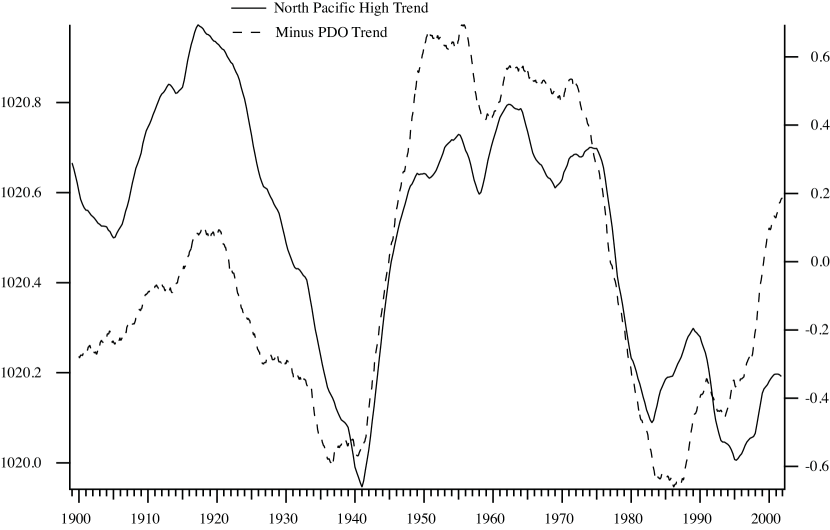
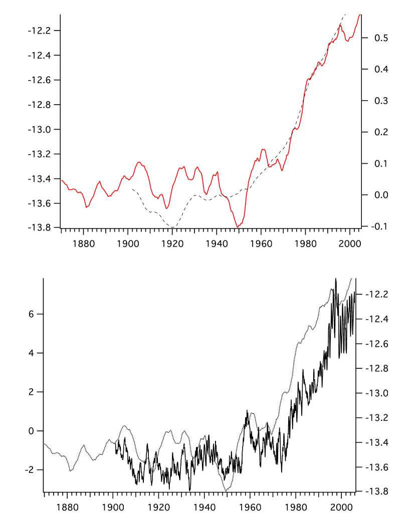
However, the trend term (Figure 1) from this analysis is almost identical to that from a state-space decomposition of sea level pressure (SLP) in the region of the North Pacific High (NPH). Physically, it would seem unlikely that the entire extra-tropical North Pacific SST is so heavily influenced by the NPH, and therefore the PDO must be reflecting only part of the variability in the region.

To properly estimate the dominant trends in the extra-tropical North Pacific SST series, and to separate these from the dominant stationary modes, requires a reanalysis of these data. In this paper, we estimate ”common trends” and ”common cycles” in the NPAC SST data using the combination of state-space decompositions and subspace identification techniques used in our previous papers (Mendelssohn and Schwing, 2002; Mendelssohn et al., 2003, 2004; Mendelssohn et al., 2005; Palacios et al., 2004) . Our results show that the trend in the original PDO discussed above is identical to the fourth common trend in our analysis, and not surprisingly the west coast of North America and the West Wind Drift region, regions that are influenced by the NPH, have the strongest weightings and are separated out in the analysis. The first common trend appears to be a ”global warming” signal, and we present evidence that it is indeed a global, rather than just a North Pacific signal.

The second common trend modifies the first common trend in areas that underwent a sharper warming (cooling) starting in the early 1970’s. The second common trend is also similar to the long-term trend in El Niño related indices identified previously in Mendelssohn et al. (2005) and to the trend in sea ice extent in the North Pacific. The first two common stochastic cycles capture what is usually thought of as the PDO and the ”Victoria” mode, explaining the strong autoregressive behavior in these indices. Finally, the higher-order common stochastic cycles suggest that large regions oscillate in contrasting patterns through time.

As a methodological note, it is often asked why bother with the more complicated state-space and subspace identification techniques instead of the usual EOF analysis. As the PDO is the first EOF of the SST series, our analysis provides a clear example that the two techniques produce different results. State-space techniques also are more powerful, as it is possible with state-space models to separate out stationary from non-stationary behavior, to examine common behavior at different time-scales, and as there is a likelihood function, to compare models and to examine residuals for adequacy of the model assumptions.

2 Data and Methods

We tried to follow as closely as possible the data processing procedures described by Mantua et al. (1997) in their analysis of the mid-latitude North Pacific Basin SST. We obtained monthly mean SST data for the years 1900 to 1993 from the U.K. Meteorological Office Global Sea Ice Coverage and SST Dataset (HadISST 1.1), which is provided by the Hadley Centre. We also obtained the monthly mean Optimally Interpolated SST (OISST.v2 Reynolds et al., 2002) data for years 1994 to present from the NOAA-CIRES Climate Diagnostics Center (http://www.cdc.noaa.gov). Both of these datasets are on a 1^∘ latitude by 1^∘ longitude grid. These datasets were then combined and averaged into 5^∘ boxes for our area of interest ; 20^∘N - 65^∘N and 110^∘E 250^∘E. We refer to boxes based on the latitude and longitude of the southwest corner, a convention used in the COADS dataset.

An index of the extent of sea ice coverage in the North Pacific was kindly provided to us by William Chapman, and extends the index reported in Chapman and Walsh (1993). This index is quarterly for the years 1900-2005.

For each of the time series a state-space decomposition was calculated, and then ”common trends” were calculated from the estimated trends and ”common cycles” from the estimated stochastic cyclic terms. A state-space model decomposition (Harvey, 1989; Durbin and Koopman, 2001), which we have applied previously to examine long-term changes in the mean and seasonal components in many other climate time series (Mendelssohn et al., 2003, 2004, and references therein) , allows for a series to be decomposed into a variety of different independent components, such as a nonparametric or fixed mean (trend), autoregressive (AR) component, stochastic cycle, stochastic seasonal, etc.:

$$y(t)=T(t)+S(t)+I(t)+e(t),\qquad t=1,\tau,$$ (1)

where, at time $t$, $T(t)$ is the unobserved time-dependent mean-level (nonparametric trend), $S(t)$ is the seasonal component (zero-mean, nonstationary and nondeterministic), $I(t)$ is the irregular term (containing any stationary autocorrelated or cyclic part of the data), and $e(t)$ is the stationary uncorrelated component, which can be viewed here as ”observation” error. This model must be more fully specified to be meaningful, which is accomplished by using piecewise continuous smoothing splines to estimate the unobserved components. Kitagawa and Gersch (1996), Harvey (1989) and Durbin and Koopman (2001) describe in detail how to parameterize the model, and solve using a combination of Kalman filtering and smoothing, and maximum likelihood estimation.

More specifically, the trend term can be viewed as a unknown function of time, and parameterized as

$$\nabla^{k}T(t)\sim N(0,\sigma_{T}^{2}).$$ (2)

The seasonal component is usually constrained in one of two fashions. In the first, the running sum of the seasonal component is constrained (assuming $s$ periods in a season)

$$\sum_{i=0}^{s-1}S(t-i)\sim N(0,\sigma_{S}^{2}),\qquad t=1,T,$$ (3)

while in the second the seasonal differences are constrained

$$S(t)-S(t-s)\sim N(0,\sigma_{S}^{2}),\qquad t=1,T.$$ (4)

The state-space specification of a stochastic cycle (Durbin and Koopman, 2001) is:

$$\left(\begin{array}[]{c}\psi_{t}\\ \psi_{t}^{*}\end{array}\right)=\rho\left(\begin{array}[]{rr}\cos\lambda_{c}&\sin\lambda_{c}\\ -\sin\lambda_{c}&\cos\lambda_{c}\end{array}\right)\left(\begin{array}[]{c}\psi_{t-1}\\ \psi_{t-1}^{*}\end{array}\right)+\left(\begin{array}[]{c}\kappa_{t}\\ \kappa_{t}^{*}\end{array}\right),\qquad t=1,\ldots,T,$$ (5)

where $\psi_{t}$ and $\psi_{t}^{*}$ are the states, $\lambda_{c}$ is the frequency, in radians, in the range $0<\lambda_{c}\leq\pi$, $\kappa_{t}$ and $\kappa_{t}^{*}$ are two mutually uncorrelated white noise disturbances with zero means and common variance $\sigma_{\kappa}^{2}$, and $\rho$ is a damping factor. The damping factor $\rho$ in (1) accounts for the time over which a higher amplitude event (consider this to be a ”shock” to the series) in the stochastic cycle will contribute to subsequent cycles. A stochastic cycle has changing amplitude and phase, and becomes a first order autoregression if $\lambda_{c}$ is $0$ or $\pi$. Moreover, it can be shown that as $\rho\rightarrow 1$, then $\sigma_{\kappa}^{2}\rightarrow 0$ and the stochastic cycle reduces to the stationary deterministic cycle:

$$\psi_{t}=\psi_{0}\cos\lambda_{c}t+\psi_{0}^{*}\sin\lambda_{c}t,\qquad t=1,\ldots,T.$$ (6)

The state-space decomposition belongs to the more general class of linear gaussian (state-space) models that are amenable to solution using the Kalman filter/smoother as:

$$y(t)&=A(t)x(t)+v(t)\\ x(t)=\Phi x(t-1)+w(t)$$ (7)

where the observation equation (Eq. 7) has $y(t)$ a $q\times 1$-vector of the observed data (in this case $q=1$), $A(t)$ is a $q\times p$ matrix which relates the data to the unobserved components $x(t)$, which is a vector of dimension $p\times 1$, and $v(t)$ is a $q\times 1$-vector of independent, identically distributed gaussian random variables with $Ev(t)=0$ and noise covariance matrix

$$R=E(v(t)v(t)^{\prime}).$$ (8)

The evolution of the unobserved components or states $x(t)$ is governed by the initial value $x(0)$ and the state equation (Eq. 7). The matrix $\Phi$ is a $p\times p$ transition matrix and the $p\times 1$-vector $w(t)$ is another independent, identically distributed gaussian random variable with $E(w(t))=0$ and

$$Q=E(w(t)w(t)^{\prime}).$$ (9)

The specification of the model is completed by assuming that $x(0)$ is also gaussian with $E(x(0))=\mu$ and

$$\Sigma=E(x(0)-\mu)(x(0)-\mu)^{\prime}.$$ (10)

See (Shumway and Stoffer, 2006, Chapter 6) for further details on the state-space model. and how the unknown parameters can be estimated using the EM algorithm.

For multivariate series, ”common trends”, ”common cycles”, and ”common seasonals” can be estimated by the appropriate specification of the transition matrix $\Phi$ and the observation matrix $A$ (see for example Harvey, 1989, ,Chapter 8). However, the computations are impractical for very large problems such as those of this paper. Instead the unobserved components are calculated using subspace identification methods (Chiuso and Picci, 2004; Hannan and Deistler, 1988; Larimore, 1996, 2000; Van Overschee and De Moor, 1996). Subspace identification methods are based on Akaike’s canonical correlation method for system identification (Akaike, 1975), and proceed by calculating the singular value decomposition of the system Hankel matrix, and then the system matrices are estimated using what are essentially multivariate least-squares procedures. Smith and Robinson (2000) and Ninness and Gibson (2000) compare the properties of the two methods for estimating linear stochastic systems and how they relate.

Subspace identification methods are usually calculated on the raw data, but as Aoki (1988) has pointed out higher frequency modes tend to have more variance, and therefore can obscure lower frequency modes. For this reason, ”common trends” were calculated by removing from each series the estimated stochastic cycle and (possibly non-stationary) seasonal terms, with similar calculations being done for the ”common cycles”.

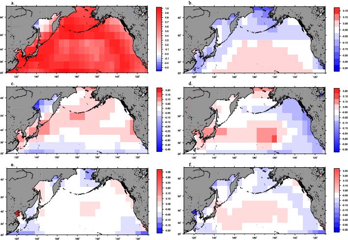
The spatial maps shown are the dynamic ”factor loadings” from the observation matrix $A$ in the Kalman filter representation of the common trends or common cycles, except for the map of the first common trend, which shows correlations instead of factor loadings because the first common trend contains a scale effect in the factor loadings - i.e. the series is not zero mean

For our models, we estimated a trend, a stochastic seasonal and a stochastic cyclic term (see Mendelssohn et al., 2005). For the original PDO index we also estimate a Markov State Switching Model (MSSM), which is often called a ”Hidden Markov Model” or HMM - see for example Hamilton (1989) or Shumway and Stoffer (1991). An MSSM extends the state-space model by assuming that there is a hidden two-regime process that switches regimes following a Markov chain, and that the parameters of the state-space model differ depending on which regime the process is in. In particular, we estimate a Markov-Switching Autoregressive Model (MSAR) that assumes that there is ”High” and ”Low” state each of which follows an AR(2) model, but the mean and parameters of the AR(2) model differ. The model is constrained such that the mean of the ”High” state can be no lower than that of the ”Low” state.

The analyses were performed using the Finmetrics package for S-Plus (Zivot and Wang, 2006). The state-space portion of this package is based on the SsfPack software developed by Koopman et al. (1999).

3 Results

3.1 Two Stationary Regimes?

The main goal of this paper is to use state-space models to re-examine the extent to which the PDO captures the dominant long-term and mid-term variability in SST in the North Pacific, but a related issue is the interpretation of the PDO as two ”stationary regimes” with the zero-crossing of the index represents the switching of the surface temperature regime in the north Pacific. The ”two-regime” interpretation implies either that the zero-crossing of the PDO has a physical meaning such that when the PDO crosses zero the rest of the ecosystem shifts, or else that embedded in the behavior of the series are two regimes with differing dynamics. Fortunately, the latter possibility can be modeled explicitly.

To examine this question further, the PDO is modeled using a Markov Switching Autoregressive Model. The model assumes that there are two regimes (a ”warm” and ”cool” regime), and an unobserved underlying process switches between the two regimes with a given probability following a Markov Chain model. Each regime is assumed to follow its own stationary AR(2) model, and the mean of the ”warm” regime is constrained to be higher than the mean of the ”cool” regime. The output includes parameter estimates for each of the AR(2) models, smoothed estimates of the probability of being in either regime, and smoothed estimates of the state of the system.

The output (Figure 2) suggests that if there were two regimes, then the Pacific was in a warm regime only from the early 1930’s to the late 1940’s, from 1956 to the early 1960’s, and from 1970 onward. However, there are reasons to prefer the state-space decomposition to the switching model. First the state-space decomposition is more parsimonious, by the AIC criterion is a better model and visually it explains the data better (particularly during periods such as 1984-1992 and after 1998). The means of the two regimes barely differ (0.028, -0.037) and the mean of the cool regime is not significantly different than zero, This suggests that a model with a single mean, such as in the state-space decomposition, is to be preferred (though there are some differences in the AR(2) model estimated for each regime, a possible asymmetry which has been noted before), which is reinforced by the fact that the smoothed state-space residuals do not show a lack of fit based on a variety of tests.

3.2 Common Trends

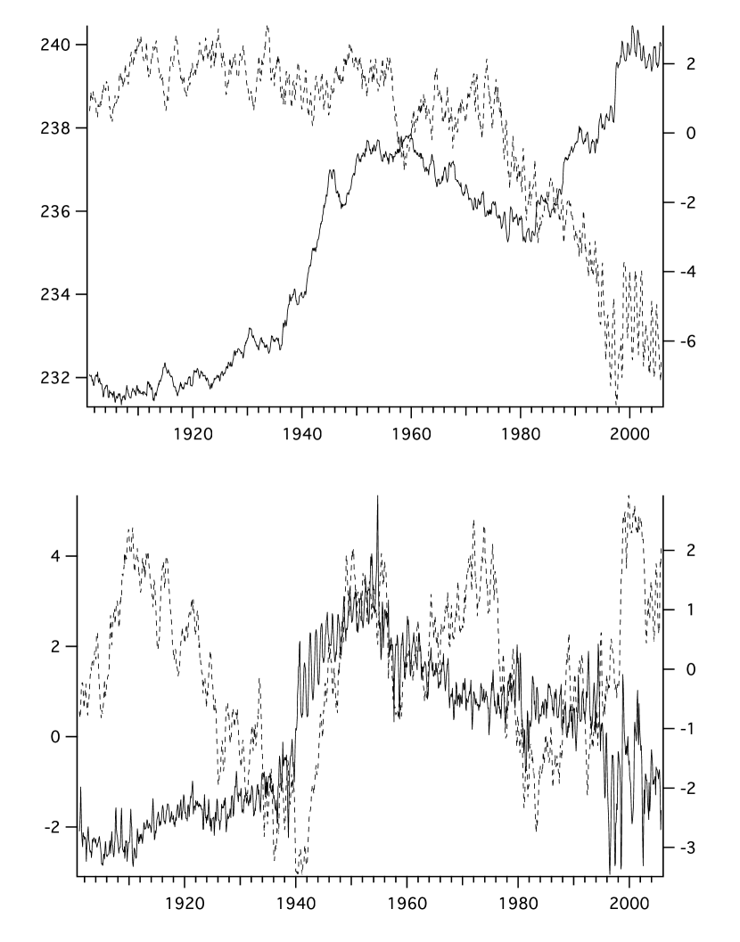
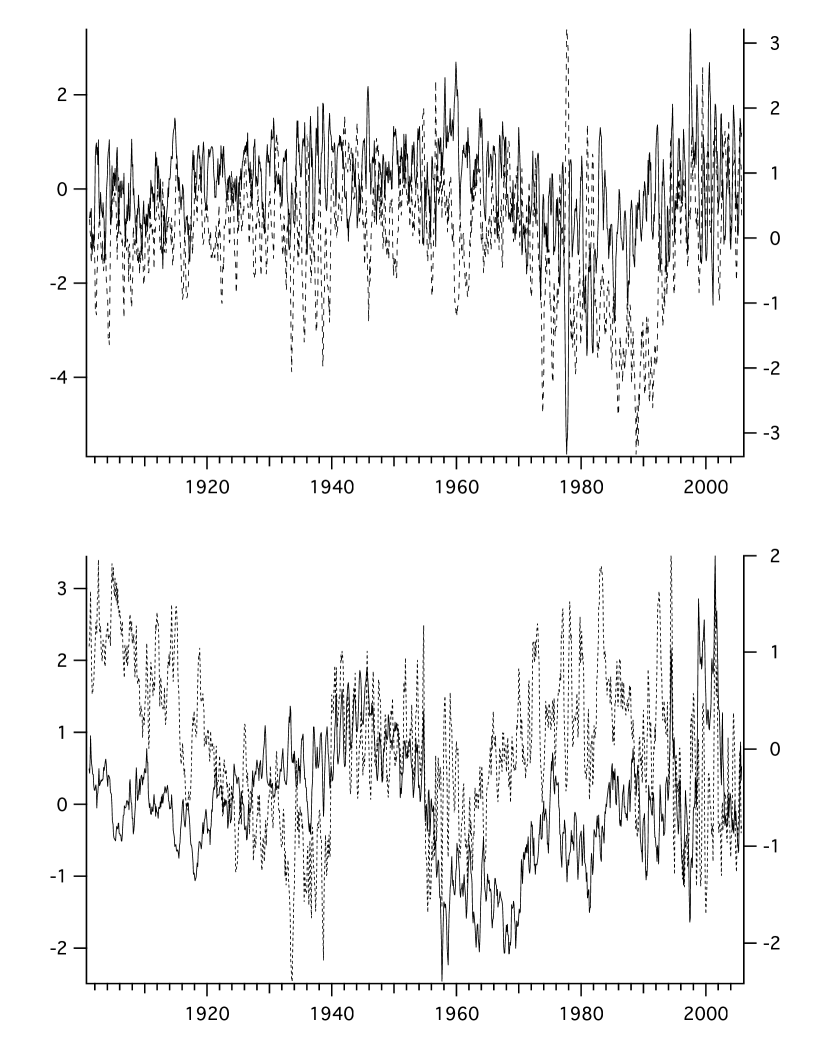
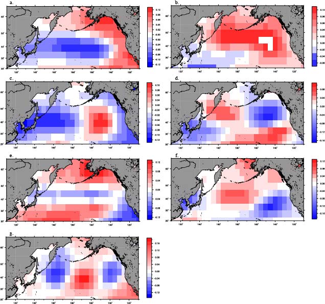
The (negative of the) first common trend ( see Figure 3 for common trends 1-4, and Figure 4 for common trends 5-8) shows a sharp increase starting in the late 1930’s to 1940 period, which reaches its maximum during 1956-1958, decreases till about 1984 and then increases to the end of the series, with an acceleration occurring in roughly 1998. The correlations between the univariate trends and the first common trend (Figure 5a) shows that the first common trend significantly correlates with the univariate trends in a band that is away from the coast or North America, crosses the Pacific between around 50^∘N-55^∘N and 20^∘N, abuts Japan but is weak in the area of the West Wind Drift and the Kuroshio Extension. The regions with significant correlations have a factor loading with absolute value in the the range of $0.10-0.07$ which translates into roughly a 0.8^∘C - 1.0^∘C change over the 100-plus years analyzed.

The second common trend (Figure 3) decreases slowly till the early 1970’s, when it declines, with the rate of decrease accelerating around 1977-78 . The significant factor loadings of the second common trend with the univariate trends (Figure 5b ) only occur in a region between 20^∘N-30^∘N and 140^∘W-160^∘E and with opposite sign in the Bering Sea. The ”1976 regime shift” (Hare and Mantua 2000; Miller et al. 1994; Trenberth 1990 ) appears to be an acceleration of a change that had already started in the North Pacific, and was most strongly expressed only in a limited area of the North Pacific, with warming in the Bering Sea area and cooling in an area closer to the tropics after 1977-1978. This is consistent with results in Schwing et al. (2007) who used state-space models to examine a variety of physical and biological data along the coast of North America, as well as some large-scale physical indices.

The first two SST common trends display significant long-term warming which appears to be accelerating in more recent years, a trend reminiscent of global warming signals. In order to see if this trend is unique to the North Pacific or is more global in scope, we compare this result with a common trend analysis of similar 5-degree SST summaries from the North Atlantic, with a common trend analysis of 23 global pressure centers, based on the data in Minobe but with the climatology restored, and with some indices of oceanographic conditions in the tropics and the Arctic.

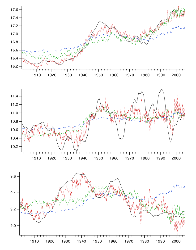
The first two SST common trends in the North Atlantic are similar to those from the North Pacific (Figure 6). The factor loadings for the North Atlantic first common trend are on the order of about .12, so that during the same 100 year period the overall increase in temperature in the North Atlantic is on the order 1.0^∘C, as in the North Pacific. Similar results hold for the second common trends.

The pressure common trend (Figure 7b) has similar change-points as does the North Pacific common trend, something first noted in Schwing et al. (2003), with tight coupling after what appears to be a major global shift around 1940. Prior to that, while both series are increasing, the rate of increase and other features of the series differ.

The (negative) of the second common trend is similar to the trend estimated by Mendelssohn et al. (2005) for the yearly Niño3 index (Figure 8) as well to the trend estimated for the sea ice extent in the Arctic, suggesting that this accelerating warming in more recent decades extends from the tropics to the Arctic. The Niño3 trend appears to start its sharp increase earlier in time, suggesting the possibility that the tropics both lead and influence the extra-tropical areas that load significantly on the second common trend. However, given that there is only one such change-point in the series, it is impossible to test if this is a real or chance relationship.

The third common trend (Figure 3) shows a sharp increase starting in 1940 till roughly 1956-1958, after which it decreases. The factor loadings (Figure 5c ) for the third common trend are most significantly positive along a portion of the west coast from central California through Washington, along the Aleutians and along Japan, and most negative in the Sea of Okhotsk and along a thin strip running roughly between 20^∘N and 22^∘N.

The univariate trends in the areas where the factor loadings are most positive (not shown) have an increase starting around 1940 that is more pronounced, and a decrease after 1956-1958 that is more rapid, than what would be predicted from the first common trend alone. These two change points align with sharp changes in the pressure centers, as shown above and in Schwing et al. (2003), and the areas with the most positive loadings are areas that would be affected by major pressure systems - for example the NPH, Western North Pacific High, and the Aleutian Low. The third common trend appears to be a superposition of a more localized pressure related change in the ocean temperatures onto the global signal represented by the first common trend.

The fourth common trend (Figure 3) loads most strongly off the west coast of North America, the west wind drift area, and off Japan, the first two being regions that should be affected by the NPH. The fourth common trend is almost identical to the trend estimated by state-space analysis of the original PDO (Figure 9). This means that the long-term dynamics of the original PDO are capturing a more localized behavior that is not the dominant long-term dynamic in the North Pacific.

The spectral behavior of the fourth common trend (Figure 10) has peaks at 52, 26 and 13 years. These periods are the harmonics of the so-called ”Seuss Wiggles” (Suess, 1965; Thomson, 1990) noticed in the analysis of ice cores, and which appear to reflect solar cycles. This suggests the very plausible link between solar cycles, changes in pressure systems in the atmosphere, and some of the variability seen in the ocean.

Common trends 5 through 8 (Figure 4) are shown for completeness. There are quasi-cyclic series whose factor loadings (Figure 5e-h) are very localized and do not represent broad-scale changes in the North Pacific. However, as we will show below, for those regions where the factor loadings are of relatively greater absolute value, these higher order common trends still play an important role in reconstructing the dynamics in those regions.

3.3 Is Variance Enough?

When studying decadal variability over a large spatial area, the main interest is often change-points or others signs of shifts in the dynamics away from what had been quasi-stationary behavior. An EOF analysis is based on the most variation in the series, while a common trends analysis attempts to find common movements in the series, which would seem most likely to correctly identify change-points and shifts.

We have shown elsewhere that when the univariate trends are reconstructed from a too low-dimension basis (say only the first or first two modes) that many important features of the original series are missed (Mendelssohn and Schwing, 2002; Mendelssohn et al., 2003), and the same is true for the North Pacific SST. The weightings of the common trends make it clear that different parts of the ocean are behaving differently, so that it is impossible to capture all of the dynamics in a very low-dimensional space. This is similar to the famous regression example of Anscombe (1973) who shows four regressions that have identical statistics, including $r^{2}$, but only one of the regressions is an adequate fit to the data. In our sub-space identification procedure the goal is to finds the smallest underlying basis that still adequately reproduces the important features of the original series.

The univariate trend at 30^∘N, 120^∘E has a correlation of $-0.975$ ($r^{2}=0.95$) with the first common trend. Despite this, if we reconstruct the univariate trend from the first common trend (Figure 11a, blue line) it severely under-estimates the sharp increase around 1950 and the large rise starting in 1992. Adding the second common trend (green line) captures these latter features, and it is not until the first three common trends are used (red line) that the original trend is reproduced. Thus, despite the extremely high correlation between the univariate trend in this region and the first common trend, reproducing the univariate trend using only the first common trend would not give an accurate impression of two of the most important features of the original trend.

In many analyses, a large number of the series have a medium level of correlation with the first mode. The univariate trend at 40^∘N, 130^∘E has a correlation of $-0.496$ ($r^{2}=0.245$) with the first common trend. The reconstruction of the univariate trend using the first common trend (Figure 11b, blue line) fails to reproduce any of the significant features of the univariate trend. Reconstructing using the first three common trends (Figure 11b, green line) captures the mean shift in the late 1930’s-1940, but not the variation around the two levels, and even using the first five common trends (Figure 11b, red line) only partially captures the variation post-1950.

As a final example, at 55^∘N, 135^∘W the univariate series has a correlation of $0.036$ ($r^{2}=0.001$) with the first common trend. This area is up in the eastern part of the Gulf of Alaska, and because of the shape of the coast, is one of the few areas in the region that is truly coastal. Mendelssohn et al. (2003) and Palacios et al. (2004) show that along the west coast of North America there is a sharp onshore-offshore gradient in almost every major feature including mixed layer depth, stratification, integrated heat content etc. at scales much smaller than the 5^∘ boxes used here, and it is questionable that any analysis using 5^∘ boxes will accurately capture coastal dynamics. This may explain why the sets of results at differing resolutions differ, and underline the fact that coastal processes may not be well represented in more broadscale analyses. This region is one of the few regions in the North Pacific with a negative correlation with the first common trend, and in fact the first common trend does a poor job of reconstructing the univariate trend (Figure 11c, blue line).

Reproducing the univariate trend from the first three common trends (Figure 11c, green line) somewhat captures the decline starting in the late 1950’s or 1960, but it is not till the first five common trends are used (Figure 11c, red line) that the dynamics of the univariate trend is well reproduced.

The reconstructions of the univariate trends in these three regions provide clear examples that variance can be misleading in determining if a mode reproduces change-points and other features of time series, and that even if a mode explains a reasonable amount of the variance, there may be large areas in the ocean that are not explained well by it. In the case of the original PDO, its trend represents two distinct regions in the North Pacific that have strong interactions with the variation in the NPH, but does not reflect the trends in the rest of the North Pacific.

3.4 Common Stochastic Cycles

The analysis of common stochastic cycles proceeds analogously to the analysis of common trends except that the stochastic cycles from the univariate state-space decompositions are used rather than the trends. Stochastic cycles, by definition, are stationary with a constant mean and covariance structure, so the dynamics of the cycles are not changing with time. These types of dynamics are somewhat separate from the main focus in this paper, the long-term, non-stationary behavior of North Pacific SST which will reflect ”climate change” and other change-points in the data. However we examine the common stochastic cycles in order to further understand the role of ”red noise” in the dynamics of NPAC SST, why Pierce (2001) and Rudnick and Davis (2003) find that the PDO is essentially red noise, and to show other well know phenomena in the Pacific region appear to be related to the stationary, rather than the non-stationary dynamics of SST..

The spatial pattern of the factor loadings for the first two common stochastic cycles (Figure 12a,b) are very similar to the spatial patterns for the original PDO and the so-called ”Victoria mode” (Bond et al. 2003) the second principal component of the SST anomalies. In fact, the first common stochastic cycle is almost identical to the stochastic cycle calculated from a state-space decomposition of the original PDO (Figure 13). Thus, while there is a ”trend” term buried in the original PDO, most of the analyses, including the spatial and temporal behavior, have focused on the stationary aspects of the PDO. Moreover, as much of the region that loads strongly on our first common cycle also loads strongly on our fourth common trend, and both include the regions that should be affected by the North Pacific High, we can see that it is this spatial overlap that produced our original state-space decomposition of the PDO. When an EOF is calculated from the anomalies, the stationary component contains more variance than does the trend term since it is at a higher frequency, and since the two regions have a high degree of overlap, the trend from this same region is indirectly included in the EOF.

The common cycles can be analyzed to ascertain the implied frequency of the term. The first common cycle has a period of 3.62 years, the second common cycle has a period of 11.4 years and the fourth common cycle has a period of 26 months. The periodicity of the first common cycle is consistent with the periods of the stochastic cycles for Darwin and Tahiti sea-level pressures estimated in Mendelssohn et al. (2005). However, for a variety of reasons, this similarity in the period of the stochastic cycle is believed due to similarity in the dynamics of the dominant pressure centers throughout the tropical and extra-tropical north Pacific, rather than the tropics driving the extra-tropical temperatures.. The period of the second common cycle is consistent with the periodicity of solar cycles, in particular sun spots, and the periodicity of the fourth common cycle is the quasi-biennial cycle. Thus the dominant stationary cyclic behavior of North Pacific SST is the occurring at the same periods as that of the atmosphere.

The spatial pattern of the factor loadings for common stochastic cycles 3-7 (Figure 12c-g) are similar to those expected from dynamics driven by spherical harmonics. The factor loadings show large spatial regions in a single direction that vary out of phase with each other as the cycle progresses through time, giving the appearance of warmer or cooler waters moving through time in that direction. For the third common stochastic cycle there are two regions out of phase in the east-west direction while the fourth common stochastic cycle also has two regions out of phase but in the southwest-northeast and northwest-southeast directions.

Similarly, for the sixth common stochastic cycle there are three regions with alternating phases in the east-west direction and for the seventh common stochastic cycle there are three regions alternating out of phase from the northwest- central-northeast regions of the Pacific. The implications of this spherical harmonic type dynamics in the North Pacific is a topic of further research.

4 Discussion and Summary

We have presented a new analysis of North Pacific SST that paints a very different picture of the long-term dynamics in this region. The ”standard” picture is based on the PDO, which we have shown that as originally calculated captures mostly the stationary, rather than non-stationary behavior of only a part of the North Pacific. The so-called ”Victoria mode” is also a stationary series that likewise reflects only part of the North Pacific. These two series are reproduced as our first two common stochastic cycles. Neither of these series represent the long-term changes in the mean or variance that we might mean when we discuss ”regime changes”, because as predominantly stationary series they have a constant mean and constant covariance structure. The changes attributed to the PDO index, as presently calculated, reflect an over-interpretation of the dynamics of autoregressive-type series, which, like lotteries, can produce regime-like behavior (long runs of numbers) without any real change in the underlying mechanism.

The long-term non-stationary dynamics estimated in our state-space analysis defines common trends that do contain important change-points that reflect changes seen in other parts of the global environment. Our first common trend behaves like a ”global warming” signal, and we show that SST in the North Atlantic have a similar first common trend, suggesting the global nature of this trend. The first common trend also displays many similarities to the first common trend from an analysis of pressure centers, and suggest that rather than 1976, both the North Pacific temperatures and the pressure systems showed changed points around 1910, around 1920, in the late 1930’s-1940, in the late 1950’s to early 1960’s , and in the period from about 1982-1984. These are the periods that appear to reflect major reorganizations in the North Pacific system, but surprisingly are hardly discussed in the literature, and for the most part agree with the analysis of abrupt changes in Schwing et al. (2003).

Our second common trend represents the ”1976 regime change” as being an acceleration of a change that had began previously (the early 1970’s) and which is an important event in the Bering Sea region and a near-equatorial band, similar to results found in Schwing et al. (2007). The second common trend also is similar to the estimated trend for the Niño3 series in Mendelssohn et al. (2005), with a suggestion of a lagged relationship between changes in the tropics and changes in these regions.

Hidden in the original PDO is a trend that is identical to the trend in the North Pacific High, and is captured as our fourth common trend. It is important in two areas, including near the coast of North America, that are strongly influenced by the NPH. This result also clarifies what has happened in the calculations of the PDO. As higher frequency dynamics usually contain higher variance than lower frequency dynamics, the PDO has captured the area that has the highest variance in the stochastic cycles, but this region mostly coincides with the region whose trend is related to the trend NPH. The fourth common trend has a spectrum with significant peaks at 52.26 and 13 years, which coincide with the so-called ”Seuss wiggles”, suggesting a solar influence to this component.

The factor loadings for common stochastic cycles 3-7 (again which are stationary) suggest wavelike (spherical harmonic) phenomena in the stochastic cycles, with large, adjacent areas of the North Pacific varying out of phase with each other as the stochastic cycles proceed. This is an important area for future research.

Finally, from a methodological standpoint, we have presented very clear evidence that the state-space techniques that we have utilized in this and other papers do produce results that differ from those produced by an EOF analysis, as the original PDO calculations are an EOF analysis of the same temperature series that we have analyzed (the EOF analysis uses the anomalies). Not just differing results, but results that have important differences in identifying when the ocean has displayed significant shifts, and what might be the dynamics causing these shifts. Moreover, the dynamics that we have estimated using state-space techniques from a wide variety of time series, from ocean temperatures to global pressures to biological data, are consistent in both temporal and spatial behaviors.

Figure 1: Comparison of (minus) the PDO trend (dashed line) with the estimated trend for the North Pacific High (solid line).

Figure 2: Results from a Markov-Switching Autoregressive Model of the PDO. The PDO (dotted line) is compared with the estimated trend from a state-space decomposition (solid line) and the smooth estimated probability of being in the warm regime (dashed line). The estimated mean of the cool regime is not significantly different from zero.

Figure 3: a). Common trend 1(solid line) and common trend 2 (dashed line). b). Common trend 3 (solid line) and common trend 4 (dashed line).

Figure 4: As in Figure 3 except for common trends 5-8.

Figure 5: a). (Negative of) correlations between the univariate trends at each location and common trend 1. b).-f). Factor loadings by location for common trends 2-6.

Figure 6: a). Comparison of the first common SST trends for the North Pacific and the North Atlantic. b).Comparison of the second common SST trends for the North Pacific and the North Atlantic

Figure 7: Comparison of the negative of common trend 1 (solid line) with common trend 1 from an analysis of 23 pressure centers in Mendelssohn et al. (2007).

Figure 8: Comparison of the negative of common trend 2 (bold solid line) with the trend for the Niño3 series (dashed line) from Mendelssohn et al. (2005) and the trend in North Pacific Sea Ice extent (light solid line).

Figure 9: Comparison of the negative of common trend 4 (solid line) with the trend for the PDO series from Mendelssohn et al. (2007).

Figure 10: Power spectrum of the fourth common trend.

Figure 11: Reconstruction of a). the univariate trend at 30N, 120E (black, $r$=-0.975) from common trend 1 (blue, common trends 1-2 (green) and common trends 1-3 (red); b). the univariate trend at 40N, 130E f(black,$r$=-0.496) from common trend 1(blue), common trends 1-3 (green), and common trends 1-5 (red); c). the univariate trend at 55N, 135W (black,$r$=0.036) from common trend 1(blue), common trends 1-3 (green), and common trends 1-5 (red). The $r$ values are the correlation between the univariate trend and common trend 1.

Figure 12: a).-f). Factor loadings by location for common cycles 1-6.

Figure 13: Comparison of the first common cycle (solid line) and the stochastic cycle estimated from a state-decomposition of the PDO

References

- Akaike (1975) Akaike, Hirotugu (1975). “Markovian Representation of Stochastic Processes by Canonical Variables.” SIAM Journal on Control and Optimization, 13: 162–173.
- Anscombe (1973) Anscombe, Francis J. (1973). “Graphs in statistical analysis.” American Statistician, pp. 17–21.
- Aoki (1988) Aoki, M. (1988). “Cointegration, error correction and aggregation in dynamic models.” Oxford Bulletin of Economics and Statistics, 50: 89–95.
- Chapman and Walsh (1993) Chapman, William L. and John E. Walsh (2012/04/08 1993). “Recent Variations of Sea Ice and Air Temperature in High Latitudes.” Bulletin of the American Meteorological Society, 74(1): 33–47. URL http://dx.doi.org/10.1175/1520-0477(1993)074<0033:RVOSIA>2.0.CO;2. doi:10.1175/1520-0477(1993)074¡0033:RVOSIA¿2.0.CO;2.
- Chiuso and Picci (2004) Chiuso, A. and G. Picci (2004). “On the Ill-conditioning of subspace identification with inputs.” Automatica, 40(4): 575–589.
- Durbin and Koopman (2001) Durbin, J. and S.J. Koopman (2001). Time Series Analysis by State-Space Methods, vol. 24 of Oxford Statistical Science Series. Oxford: Oxford University Press.
- Hamilton (1989) Hamilton, James D (1989). “A New Approach to the Economic Analysis of Nonstationary Time Series and the Business Cycle.” Econometrica, 57(2): 357–384. URL http://www.jstor.org/stable/1912559.
- Hannan and Deistler (1988) Hannan, E.J. and M. Deistler (1988). The Statistical Theory of Linear Systems. New York: John Wiley and Sons.
- Harvey (1989) Harvey, Andrew C. (1989). Forecasting, structural time series models and the Kalman filter. Cambridge University Press.
- Kitagawa and Gersch (1996) Kitagawa, G. and Will Gersch (1996). Smoothness Priors Analysis of Time Series. Springer-Verlag Inc.
- Koopman et al. (1999) Koopman, Siem Jan, Neil Shephard and Jurgen A. Doornik (1999). “Statistical algorithms for models in state space using SsfPack 2.2.” Econometrics Journal, 2(1): 107–160. URL http://ideas.repec.org/a/ect/emjrnl/v2y1999i1p107-160.html.
- Larimore (1996) Larimore, W. E. (1996). “Statistical Optimality and Canonical Variate Analysis System Identification.” Signal Processing, 52: 131–144.
- Larimore (2000) — (2000). “Identification of Colinear and Cointegrated Multivariable Systems Using Canonical Variate Analysis.” In Symposium on System Identification 2000. Santa Barbara, CA.
- Mantua et al. (1997) Mantua, N. J., S. R. Hare, Y. Zhang, J. M. Wallace and R. C. Francis (1997). “A Pacific interdecadal climate oscillation with impacts on salmon production.” Bulletin of the American Meteorological Society [Bull. Am. Meteorol. Soc.], 78(6): 1069–1080.
- Mendelssohn et al. (2005) Mendelssohn, R, SJ Bograd, FB Schwing and DM Palacios (APR 12 2005). “Teaching old indices new tricks: A state-space analysis of El Nino related climate indices.” Geophysical Research Letters, 32(7). doi:10.1029/2005GL022350.
- Mendelssohn and Schwing (2002) Mendelssohn, R. and F.B. Schwing (2002). “Common and uncommon trends in SST and wind stress in the California and Peru-Chile Current Systems.” Progress in Oceanography, 53(2-4): 141–162.
- Mendelssohn et al. (2003) Mendelssohn, R., F.B. Schwing and S.J. Bograd (2003). “Spatial structure of subsurface temperature variability in the California Current, 1950-1993.” Journal of Geophysical Research, 108(C3): 3093, doi:10.1029/2002JC001568.
- Mendelssohn et al. (2004) — (2004). “Nonstationary Seasonality of Upper Ocean Temperature in the California Current.” Journal of Geophysical Research, 109((00)): C10015,doi:10.1029/2004JC002330.
- Mendelssohn (2011) Mendelssohn, Roy (5 2011). “The STAMP Software for State Space Models.” Journal of Statistical Software, 41(2): 1–18. URL http://www.jstatsoft.org/v41/i02.
- Ninness and Gibson (2000) Ninness, B. and S. Gibson (2000). On the Relationship Between State- Space-Subspace Based and Maximum Likelihood System Identification Methods.. Technical Report EE20021, Department of Electrical and Computer Engineering, University of Newcastle, Australia.
- Palacios et al. (2004) Palacios, Daniel M., Steven J. Bograd, Roy Mendelssohn and Franklin B. Schwing (2004). “Long-term and seasonal trends in stratification in the California Current, 1950-1993.” Journal of Geophysical Research, 000((00)): 000,doi:10.1029/2004JC002380.
- Pierce (2001) Pierce, DW (2001). “Distinguishing coupled ocean-atmosphere interactions from background noise in the North Pacific.” Progress in Oceanography, 49(1-4, Sp. Iss. SI): 331–352.
- Reynolds et al. (2002) Reynolds, Richard W., Nick A. Rayner, Thomas M. Smith, Diane C. Stokes and Wanqiu Wang (2012/04/08 2002). “An Improved In Situ and Satellite SST Analysis for Climate.” Journal of Climate, 15(13): 1609–1625. URL http://dx.doi.org/10.1175/1520-0442(2002)015<1609:AIISAS>2.0.CO;2. doi:10.1175/1520-0442(2002)015¡1609:AIISAS¿2.0.CO;2.
- Rudnick and Davis (2003) Rudnick, DL and RE Davis (JUN 2003). “Red noise and regime shifts.” Deep-Sea Research Part I-Oceanographic Research Papers, 50(6): 691–699. doi:10.1016/S0967-0637(03)00053-0.
- Schwing et al. (2003) Schwing, F.B., J. Jiang and R. Mendelssohn (2003). “Coherency of multi-scale abrupt changes bewteen the NAO, NPI, and PDO.” Geophysical Research Lettere, 30(7): 1406, doi:10.1029/2002GL016535.
- Schwing et al. (2007) Schwing, F.B., R. Mendelssohn and S.J. Bograd (2007). “When did the 1976 regime shift occur? Paradigm lost.” Unpublised Manuscript.
- Schwing et al. (2010) Schwing, Franklin B, Roy Mendelssohn, Steven J Bograd, James E Overland, Muyin Wang and Shin-ichi Ito (2010). “Climate change, teleconnection patterns, and regional processes forcing marine populations in the Pacific.” Journal of Marine Systems, 79(3-4): 245–257. URL http://linkinghub.elsevier.com/retrieve/pii/S0924796309000827.
- Shumway and Stoffer (1991) Shumway, R. H. and D. S. Stoffer (1991). “Dynamic linear models with switching (Corr: V87 p913).” Journal of the American Statistical Association, 86: 763–769.
- Shumway and Stoffer (2006) Shumway, Robert H. and David S. Stoffer (2006). Time Series Analysis and Its Applications: With R Examples [Second Edition]. Springer Texts in Statistics. New York: Springer-Verlag.
- Smith and Robinson (2000) Smith, G.A and A.J. Robinson (2000). A Comparison Between the EM and Subspace Identification Algorithms For Time-Invariant Linear Dynamical Systems.. Technical Report CUED/F-INFENG/TR.345, Engineering Department, Cambridge University, England.
- Suess (1965) Suess, Hans E. (1965). “Secular Variations of the Cosmic-Ray-Produced Carbon 14 In the Atmosphere and Their Interpretations.” J. Geophys. Res., 70(23): 5937–5952. URL http://dx.doi.org/10.1029/JZ070i023p05937. doi:10.1029/JZ070i023p05937.
- Thomson (1990) Thomson, D. J. (1990). “Time Series Analysis of Holocene Climate Data.” Philosophical Transactions of the Royal Society of London. Series A, Mathematical and Physical Sciences, 330(1615): 601–616. URL http://rsta.royalsocietypublishing.org/content/330/1615/601.abstract. doi:10.1098/rsta.1990.0041.
- Van Overschee and De Moor (1996) Van Overschee, P. and B. De Moor (1996). Subspace Identification for Linear Systems: Theory-Implementation-Application. Dordrecht: Kluwer-Academic Publisher.
- Zivot and Wang (2006) Zivot, E. and J. Wang (2006). Modeling Financial Time Series With S-Plus. No. v. 13 in Modeling Financial Time Series with S-PLUS. Springer. URL http://books.google.com/books?id=sxODP2l1mX8C.