Rotation-stimulated structures in the CN and C₃ comae of comet 103P/Hartley 2 around the EPOXI encounter

Abstract

Context. In late 2010 a Jupiter Family comet 103P/Hartley 2 was a subject of an intensive world-wide investigation. On UT October 20.7 the comet approached the Earth within only 0.12 AU, and on UT November 4.6 it was visited by NASA EPOXI spacecraft.

Aims. We joined this international effort and organized an observing campaign with three key goals. First, to measure the parameters of the nucleus rotation in a time series of CN. Second, to investigate the compositional structure of the coma by comparing the CN images with nightly snapshots of C₃. And third, to investigate the photochemical relation of CN and HCN, using the HCN data collected nearly simultaneously with our images.

Methods. The images were obtained through narrowband filters using the 2-m telescope of the Rozhen National Astronomical Observatory. They were taken during 4 nights around the moment of the EPOXI encounter. Image processing methods and periodicity analysis techniques were used to reveal transient coma structures and investigate their repeatability and kinematics.

Results. We observe shells, arc-, jet- and spiral-like patterns, very similar for the CN and C₃ comae. The CN features expanded outwards with the sky-plane projected velocities between 0.1 to 0.3 km s^-1. A corkscrew structure, observed on November 6, evolved with a much higher velocity of 0.66 km s^-1. Photometry of the inner coma of CN shows variability with a period of 18.32$\pm$0.30 h (valid for the middle moment of our run, UT 2010 Nov. 5.0835), which we attribute to the nucleus rotation. This result is fully consistent with independent determinations around the same time by other teams. The pattern of repeatability is, however, not perfect, which is understendable given the suggested excitation of the rotation state, and the variability detected in CN correlates well with the cyclic changes in HCN, but only in the active phases. The revealed coma structures, along with the snapshot of the nucleus orientation obtained by EPOXI, let us estimate the spin axis orientation. We obtained RA=122°, Dec=+16° (epoch J2000.0), neglecting at this point the rotational excitation.

1 Introduction

103P/Hartley 2 (hereafter 103P) is a Jupiter Family comet, which currently has a perihelion at 1.06 AU and orbits the Sun with a 6.47-year period. Due to frequent perihelion passages, the comet was relatively well characterised prior the 2010 apparition (see e.g. Arpigny at al. arpigny93 (1993); Weaver et al. weaver94 (1994); Crovisier et al. crovisier99 (1999); Colangeli et al. colangeli99 (1999); Epifani et al. epifani01 (2001)), although no information about the nucleus rotation was obtained.

The state of rotation is, however, of great interest, because it is one of the parameters which establish the lifetime of a comet nucleus. It has been realised long ago, that a nucleus rotating faster than a certain limit (see e.g. Davidsson davidsson01 (2001)) must be disrupted by a centrifugal force. On the other hand, knowledge of this parameter enables proper interpretation of the observational data and their conversion to the physical quantities (such as the total production rates and relative abundances) which can be compared among comets.

The rotation period of 103P was first measured at 16.4$\pm$0.2 h (Meech et al. meech11 (2011)) shortly after the comet was selected as the target of NASA EPOXI mission. The studies on the rotation continued when the comet became active. EPOXI-based imaging and photometry (A’Hearn et al. ahearn11 (2011)), as well as ground-based observations (see Meech et al. meech11 (2011) for an overview of the ground-based results), show that the rotation period was increasing with time and that the nucleus most probably was rotating in excited mode.

Although indications of possible changes in the spin rate among comets have been reported before for some objects (e.g. C/1990 K1 (Levy), C/2001 K5 (LINEAR), 2P/Encke, 6P/d’Arrest, 10P/Tempel 1), the first unequivocal measurement of a slow decrease of the rotation period was obtained only recently for comet 9P/Tempel 1 (Belton & Drahus belton07 (2007); Belton et al. belton11 (2011)). Model computations (e.g. Gutiérrez et al. gutierrez03 (2003)) show that emission of matter from active vents occupying small fraction of an irregularly-shaped rotating nucleus can produce a significant net torque. Due to this effect cometary rotation can evolve from the principal-axis toward the non-principal-axis (excited) mode after a couple of perihelion passages and remain in this state during the next tens of orbital revolutions. The problem of rotational excitation is important for the long-term evolution of cometary nuclei as the relaxation timescale has not been well established to date (e.g. Samarasinha et al. samarasinha04 (2004)). Despite the suggestion made by some authors (e.g. Belton belton91a (1991); Jewitt jewitt92 (1992)) that most short-period comets should be in excited spin states, only a couple of such cases have been reported before: 2P/Encke (Belton et al. belton05 (2005)), 29P/Schwassmann-Wachmann 1 (Meech et al. meech93 (1993)), and 1P/Halley (Belton et al. belton91b (1991)). The recent results on 103P show that its nucleus – having been observed in an excited and decelerated rotation state – is the first known comet in which the two processes occur at the same time. Moreover, thanks to the EPOXI mission, which provided detailed characteristics of the nucleus, this exceptional object is a unique laboratory to test our theories about the rotational dynamics of cometary nuclei.

Impressive images of 103P’s nucleus obtained by EPOXI (A’Hearn et al. ahearn11 (2011)) show an elongated body with tips of different sizes, the smaller one being insolated and active at the encounter. The nucleus is found to precess about the longest axis of inertia with the period of 18.34$\pm$0.04 h and roll about the shortest axis of inertia (longest nucleus extent) with the probable period of 27.79$\pm$0.31 h (both at the epoch of the EPOXI encounter). The two periodicities are nearly commensurate in 2:3 resonance which causes the activity pattern to repeat every three precession cycles – the characteristic observed also in ground-based HCN data (Drahus et al. drahus11 (2011)).

In this work we analyse transient features in the CN and C₃ comae. In particular, the time series of CN is used to examine the kinematics, repeatability, and periodicity in the framework of the nucleus precession-roll scenario. We also determine the spin axis orientation of the nucleus. Our campaign was realized simultaneously with the HCN monitoring at IRAM 30-m (Drahus et al. drahus11 (2011); drahus12 (2012)), which makes it possible to investigate the connection between HCN and CN. Although the HCN molecule is considered as the main donor of cometary CN (e.g. Bockelée-Morvan & Croviser bockelee85 (1985)), the issue is still somewhat controversial (e.g. Fray et al. fray05 (2005)).

2 Observations and data reduction

Observations of 103P were carried out on four photometric nights: November 2, 4, 5 and 6, 2010, including the date (though not the moment) of the EPOXI encounter. The last night before the encounter, i.e. November 3, 2010, was also allocated but lost due to bad weather. We observed with the two-channel FoReRo2 focal reducer (Jockers et al. jockers00 (2000)) mounted in the Cassegrain focus of the 2-m Ritchey-Chrétien-Coudé telescope of the Rozhen National Astronomical Observatory (Bulgarian Academy of Sciences). In the blue channel we used Photometrics CE200A-SITe, and in the red channel VersArray 512B. Both CCDs have square-shaped 24-$\mu$m pixels, and give the image scale of 0.89 arcsec pix^-1, i.e. $\sim$100 km at the comet nucleus.

In this work we present the results of imaging in the blue channel and the other data will be presented in a subsequent paper. Emission bands of CN and C₃ were observed through the HB filters (Farnham et al. farnham00 (2000)) at 387 nm and 406 nm respectively; dust was observed through an interference filter at 443 nm. All exposures were 600 s with non-sidereal tracking on the comet. We obtained a couple of hours long series of CN images and snapshots of C₃ and dust. Reduction of the images included, in addition to the standard steps, removal of Cosmic Ray Hits (CRH) and stellar profiles. We stacked consecutive images in pairs and cleaned them using the procedure described in Appendix A. In this way we obtained 31 clean stacks for CN, 7 for C₃ and 7 for dust. The mid-exposure moments for the co-added images have been corrected for the travel time of light. The statistics of the observations and the geometric circumstances, are presented in Table 1.

Table 1: Statistics of the images and geometric circumstances

UT Date	$r$ a	$\Delta$ b	$\phi$ c	Number of exposures d
Nov. 2010	[AU]	[AU]	[∘]	CN         C3      dust
2.96 – 3.10	1.062	0.150	58.7	11/6       2/1     4/2
4.94 – 5.16	1.064	0.158	58.8	20/10    4/2      2/1
5.93 – 6.16	1.066	0.163	58.8	17/9       3/2      3/2
6.96 – 7.17	1.067	0.167	58.7	11/6       3/2      3/2

• Heliocentric distance

• Topocentric distance

• Topocentric phase angle (i.e. Sun-comet-observer angle)

• Numbers of original/stacked images.

To enhance the visibility of faint coma structures we proceeded in a similar way as for comet 8P/Tuttle (Waniak et al. waniak09 (2009)). This approach assumes and critically depends on constant heliocentric distance of the comet and constant observing geometry in the analysed set of images – the conditions which are well satisfied for our short run (see Table 1). In such a case, the only reason for coma variability can be transient phenomena produced by e.g. unstable and/or periodically changing mass ejection. First, we converted the scales of the individual stacked images to the same topocentric distance for UT 2010 Nov. 5.0. Then a series of the rescaled frames for a given filter was used as an input to our novel technique: the Iterative Image Decomposition, which extracts the time-invariant coma profile, and produces a series of images for the residual, time-dependent component. Our iteration loop contains two steps: (i) rescaling image signal by a factor followed by (ii) stacking such modified images into a mean frame. The normalization factors are adjusted with respect to this mean frame taken as a reference. The procedure begins with stacking of the original input frames with no normalization (i.e. the factors set equal to unity). In the subsequent iterations we stacked not the whole images but only the parts that do not change their profiles from frame to frame. These stable parts made it possible to comput the factors for signal rescaling. To detect and avoid pixels containing signatures of temporary signal enhancement we applied the $K\sigma$ criterion for the pixel value difference between the individual normalised frame and the mean image. After a number of iterations, when the mean profile appeared stable, we took this profile as the time-invariant coma pattern and subtracted it from the individual, normalised input frames, obtaining a series of residual images. Our experience shows, that such images are photometrically linked to a much better precision than can be achieved when linking through standard stars and nightly extinction coefficients. This approach has also other advantages over typical image enhancement procedures. It generally preserves photometric information, so the transient structures can be analysed quantitatively. Moreover, the level of enhancement does not depend on position, shape or size of a feature, if only the area of this feature is significantly smaller than the total area of the analysed part of the coma, and if the series of input images sufficiently samples the time variability of the coma profile.

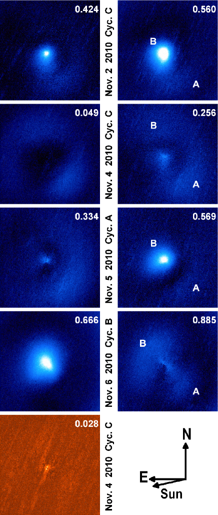
Figure 1: First and last residual image of CN for each night. The bottom left panel shows the typical residual image of the dust coma. Dates and cycles (see text for details) are displayed. Phases with respect to the 18.32 h cycle are shown in the upper-right corners. The field of view is 6.4 arcmin or 43.8$\times$10³ km at the nucleus.

As we did not subtract the light scattered by cometary dust from the signal in the molecular filters, it is obvious that our CN and C₃ images still contain dust contribution. This contribution is very weak, though, as 103P has a very low dust-to-gas ratio (Schleicher schleicher10 (2010)). Furthermore, the dust images processed with our Iterative Image Decomposition, show no transient structures (see Fig. 1). This means that the signal contribution from dust is totally contained in the stationary CN and C₃ profiles, and therefore the residual images contain pure information about the variability of the molecular coma.

3 CN and C₃ transient structures

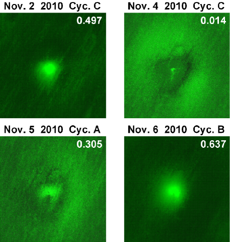
Figure 2: Images of C₃ obtained by stacking the nightly series of the residual frames to increase the $S/N$ ratio. Dates and cycles (see text for details) are displayed above the frames. Phases with respect to the 18.32 h period are shown in the upper-right corners. Orientation and image scale are the same as in Fig. 1.

Our residual images for CN and C₃ show the evolution of the transient structures during 4 nights between November 2 and November 6. Part of the whole set for CN is presented in Fig. 1 (the complete, chronologically ordered series can be seen as a video clip Animation1). To show how the CN coma evolved with time, in Fig. 1 we present the first (left column) and last (right column) residual image for each night. In Fig. 2 we show nightly-averaged snapshots for C₃.

Figures 1 and 2 reveal transient features of different kinds, and show that the CN and C₃ structures fully correlate. This means that both molecular environments behaved in very similar ways. To analyse the coma evolution with time we introduced the nomenclature used earlier by Drahus et al. (drahus11 (2011)). Each residual frame corresponds to a given precession phase (changing from 0 to 1) and precession cycle (denoted as A, B, and C) of the threefold precession period (the three-cycle period). The phases are obtained using the precession period of 18.32 h (justified further in Section 5). The moment of the EPOXI encounter occurred at the precession phase of 0.5 at the middle of Cycle B.

As can be seen in Fig. 1, our data cover almost the full precession cycle. During the four nights we observed Cycles C, C, A and B, respectively. Although we covered all the three cycles, we never observed the same cycle and phase twice. In general, we notice markedly enhanced CN production at phases close to 0.5 on November 2, 5 and 6, when the central shells appeared and brightened on November 2 and 5, and diminished on November 6. These shells expanded outward, bearing arc- and spiral-like structures, which are visible up to the early phases of the next cycles. The shape and temporal evolution of the structure from November 6 resembles a traditional corkscrew (cf. Fig. 1 and Animation1): the north-east part can be identified as a relatively massive handgrip and the narrower south-west pattern can be attributed to the spiral (although its actual spirality is not visible due to projection onto the sky). Such corkscrew patterns have also been reported for 103P earlier (Knight & Schleicher knight11 (2011); Samarasinha et al. samarasinha11 (2011)).

Even a simple analysis reveals that all the three central shells have different profiles and behave differently in time. This can can be seen in video clip Animation2, where we applied a technique similar to ring-masking (A’Hearn et al. ahearn86 (1986)) to the residual images, to additionally enhance the contrast in the central region (from the individual pixel values our method subtracts the smoothed radial profile of the azimuthal minimum). The features in the outer coma poorly correlate with their progenitors visible during the earlier cycles, which can be caused by the postulated excitation of the rotation state.

4 Kinematics of the CN features

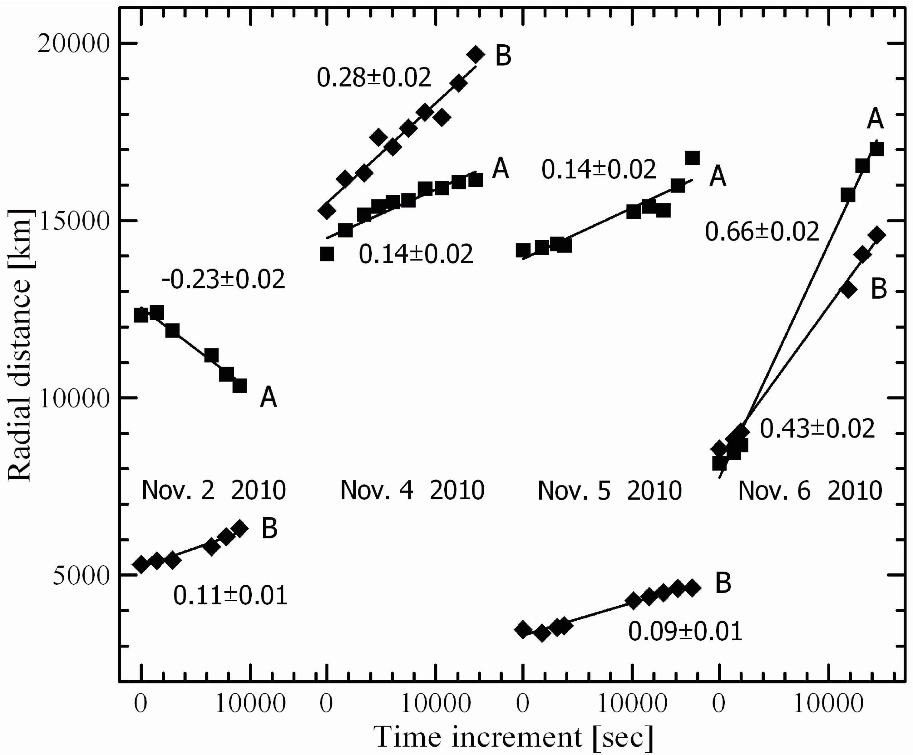
Figure 3: Relation between the radial distances of the CN structure and time. The error bars are of the order of the symbol size and have been omitted. Linear fits and the expansion velocities in km s^-1 are displayed.

To shed more light on the nature of the transient structures we have investigated their kinematics. The expansion velocity of the shells and arcs was measured separately in the south-west (A) and north-east (B) quadrants, as labeled in Fig. 1. We proceeded in a similar way as in our earlier work on 8P/Tuttle (Waniak et al. waniak09 (2009)). First, we transformed the CN residual images to the rectangular frames arranging the radial distance from the nucleus in columns and the azimuth angle in rows. Then for every pair of such images from a given night, we determined the radial shift of the transient feature between both images. We cross-correlated the two frames, using a range of different displacements in the radial distance, to find the maximum of the correlation coefficient. Our approach ensures a sub-pixel precision of the shift determination even for diffuse features, but it does not return the radial distance itself. Using the radial increments for all the pairs of residual images from each night and the radial distance of the chronologically first position from a crude estimation, we computed (using LSQ approach) the radial distances of the succeeding positions of a given CN structure. The retrieved positions are presented in Fig. 3 together with the expansion velocities projected onto the sky plane, obtained from a linear fit.

In general, the projected velocities of different features are much smaller than the expansion velocity of 1.0 km s^-1, considered as canonical for the gas coma at 1 AU (e.g. Combi et al. combi04 (2004)). For November 2, 4 and 5 they range between 0.1 and 0.3 km s^-1, except for arc A on November 2, which exhibited movement toward the coma centre with the velocity of 0.23 km s^-1. This unusual arc does not correlate with any other arc- or spiral-like feature visible in Fig. 1. As the nature of this phenomenon remains unlear at the moment, we leave it for the subsequent model analysis.

As has been shown by Waniak et al. (waniak09 (2009)), CN produced by photodissociation of HCN is a good tracer of its parent for the radial distances up to about one photochemical scalelength of HCN. Since the maximum radial distance considered in our analysis ($\sim$2$\times$10^-4 km) is only twice the scalelength for HCN ($\sim$10^-4 km), the condition is reasonably satisfied. Hence, the CN expansion velocity has to correlate well with the HCN expansion velocity. Obviously, it is hard to imagine that the expansion of the gas coma in 103P was indeed as slow as the projected expansion of the CN structures. The projection effect would be negligible only if we observed expansion of a spherical shell or if the structures were exactly in the sky-plane. The real expansion velocity was most probably significantly reduced by the on-sky projection indicating mass loss into a cone with a given opening angle and orientation. The November 6 data revealed a much higher expansion velocity of 0.66 km s^-1 for arc A and 0.43 km s^-1 for arc B, which can be possibly explained by a significantly changed geometry of the gas ejection, resulting in a strong reduction of the projection effect.

5 Periodicity in the CN data

The CN residual images were used as an input time series to search for periodicity. We separately investigated (i) variability in the photometric signal, and (ii) repeatability of the transient features.

First, we performed aperture photometry of the central region of the CN coma, using a diaphragm with the optimum, 12-arcsec diameter (increasing the diaphragm size would result in a higher level of undesirable smoothness and phase delay of the near nucleus signal variability, but decreasing the diameter would cause a higher noise pollution of the photometric data and greater influence of imperfect on-comet tracking, variable seeing, and defocus). We checked that the diaphragm twice as small changes the behaviour of the photometric data negligibly. That is because the expected aperture effect is stifled by the phase delay introduced by the photodissociation of the CN parent. The timescale for the aperture effect (i.e., the travel time between the aperture centre and its edge) is of the order of 10³ s and the typical photodissociation timescale for the CN parent at 1 AU heliocentric distance is of the order of 10⁴ s.

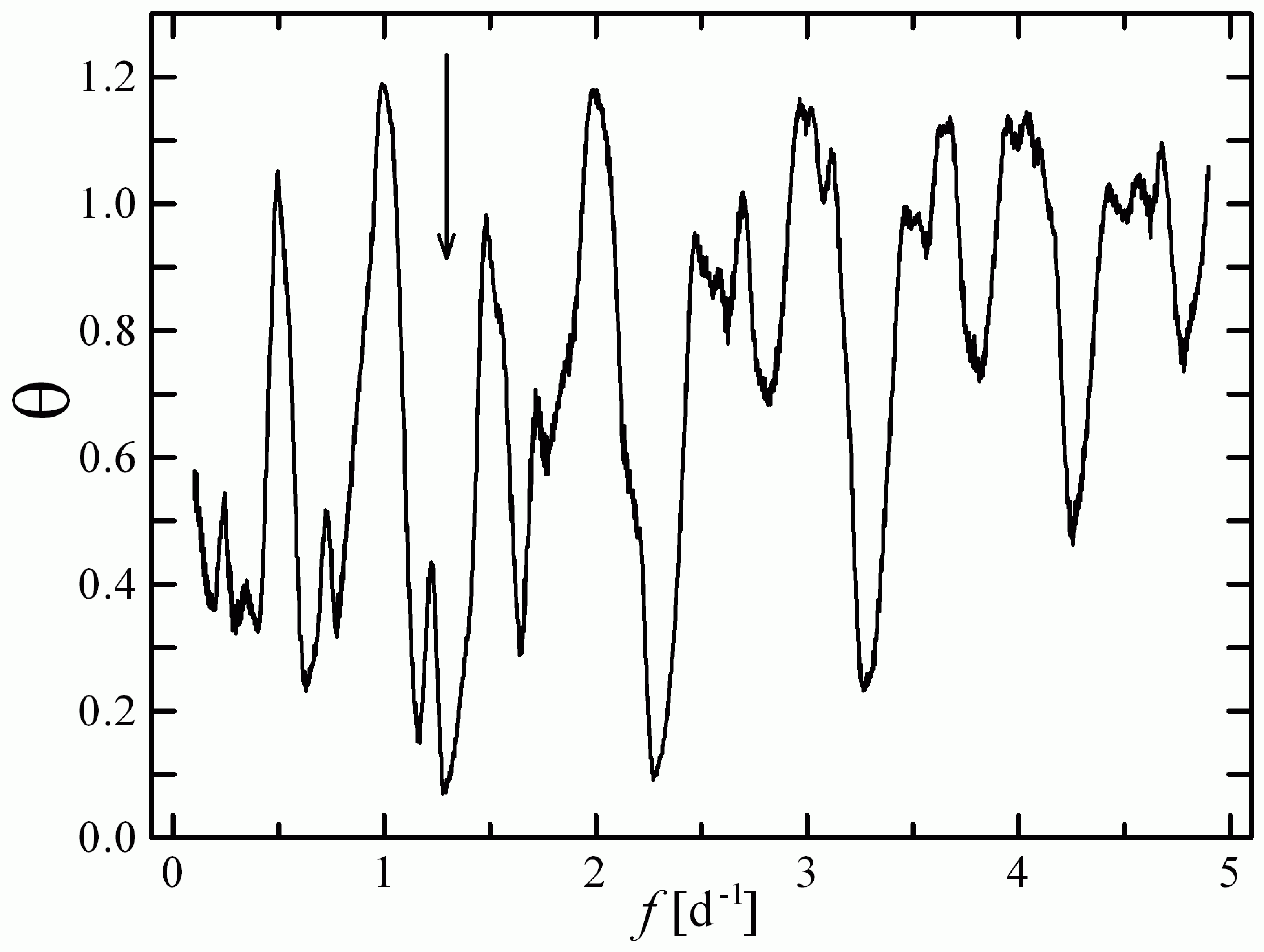
Figure 4: PDM periodogram for our photometric data calculated using 6 bins and 6 covers. The optimal solution is found at the frequency of 1.310 d^-1 (period of 18.32 h) and is pointed by an arrow.

The periodicity was investigated using the weighted version of the Phase Dispersion Minimization (PDM), developed by Drahus & Waniak (drahus06 (2006)) from the classical non-weighted PDM (Stellingwerf stellingwerf78 (1978)). Quality of data phasing is probed by a parameter $\theta$, which is a ratio of variances of the phased and unphased data. The resulting PDM periodogram is presented in Fig. 4. The global minimum of $\theta$ occurs at the periodicity of 18.32$\pm$0.30 h. Other minima are produced by the interference with a one-day cycle or represent harmonics of the basic frequency. Our result is an instantaneus synodic rotation period for the epoch UT 2010 Nov. 5.0835, i.e. for the middle moment of our run. Compared to other results obtained for similar dates, our solution is the same as the 18.32$\pm$0.03 h periodicity detected in the HCN data (Drahus et al. drahus11 (2011)), agrees within the errors with the periods of 18.34$\pm$0.04 h from the EPOXI photometry (A’Hearn et al. ahearn11 (2011)) and 18.195$\pm$0.010 h obtained from radar Doppler imaging (Harmon et al. 2011a ), and is similar to 18.7$\pm$0.3 h (Knight & Schleicher knight11 (2011)) and $\sim$18.8 h (Samarasinha et al. samarasinha11 (2011)) inferred from the repeatability of the CN coma profile.

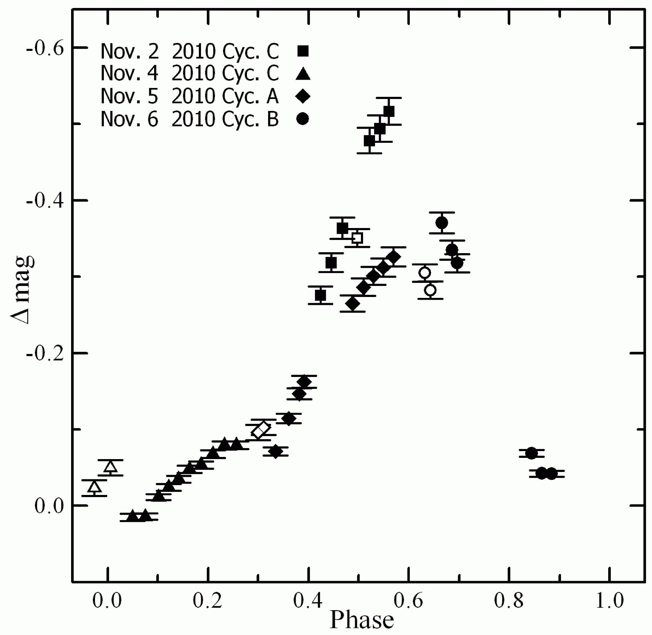
Figure 5: Molecular light curves for CN (filled symbols) and C₃ (open symbols) phased according to the 18.32 h period. The moment of the EPOXI encounter has a phase 0.5 of Cycle B.

The light curve phased according to the period of 18.32 h is displayed in Fig. 5, where we show a magnitude difference between the residual frames and the time-invariant average coma profile produced by the Iterative Image Decomposition. Since the latter can be contaminated by dust (in contrast to the residual images; cf. Section 2), the presented light curve can be slightly deformed. For comparison, the C₃ photometric data are also presented in this plot. Although the C₃ signal could be contaminated by dust more strongly than CN, the photometric variability is comparable for both radicals. The maxima of the CN signal visible close to phase 0.5 can be linked with periodical insolation of the smaller tip of the elongated nucleus, that was active during the EPOXI encounter. Figure 5 shows that the maximum levels of the CN signal most probably differ noticeably for Cycles A, B, and C. The secondary increase of the CN signal at phases $\sim$0.25 of Cycle C (November 4) is related to the weak central enhancement (see Fig. 1) and could be attributed to less active vents.

Another approach to investigate the periodicity in our residual images of CN is analysis of repeatability of the CN transient structures based on cross-correlation of the patterns in the residual frames. It is independent of the signal and measures the real similarity of the profiles. Although this procedure uses a different parameter than we used in the earlier work on comet 8P/Tuttle, the philosophy behind did not change, and can be found in Waniak et al. (waniak09 (2009)). Because the outer CN structures, detached from the central features, present diversity of profiles and expansion velocities, we have compared only the central features visible on November 2, 5 and 6. The resulting set of the cross-correlation parameters related to the time increments between two exposures is presented in Fig. 6.

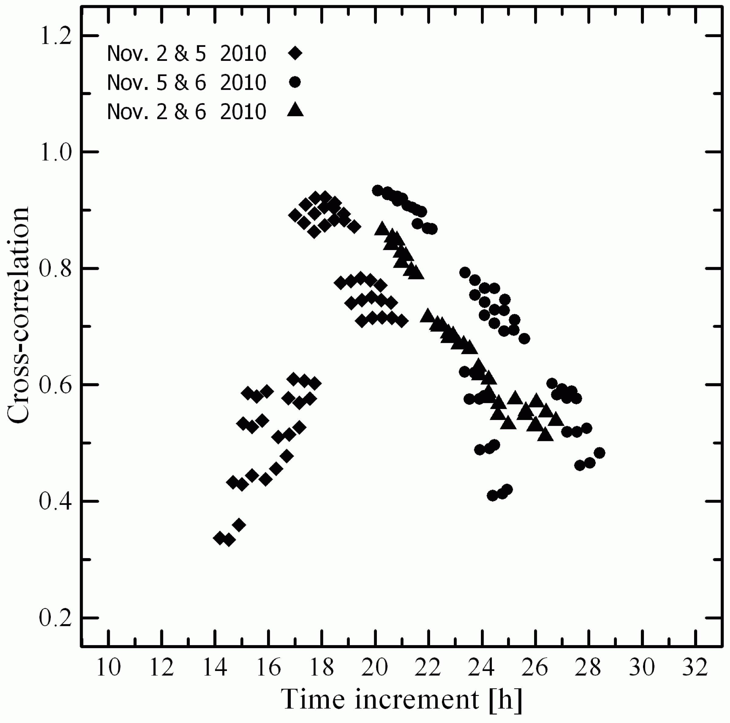
Figure 6: Cross-correlation of the central CN shells between three nights. Multiples of the 18.32 h period have been subtracted from the actual time increments to obtain differences closest to the single period.

Unfortunately, none of the dependencies characterising the three pairs of nights present a clear maximum that could be used to precisely measure the period. While the plot is not as convincing as the photometric result in Fig. 5, it nevertheless provides an independent confirmation of our solution. Worth noticing are the relatively high levels of cross-correlation, reaching up to 0.95 for November 2 and 5, and November 5 and 6. Even though the central shells observed on November 2, 5 and 6 look differently at first sight (see Fig. 1), the quantitative analysis shows that in general the patterns are similar.

6 Differences between the nucleus precession cycles

First, we compare the behaviour of the CN coma in three consecutive precession cycles: Cycle A, B, and C, which we observed during the production-rate maxima on November 2 (Cycle C), 5 (Cycle A) and 6 (Cycle B). After analysing the behaviour of the central CN shells in the residual images (Fig. 1), and taking into account that we showed (Fig. 6, Section 5) a higher correlation level for the pairs of nights November 2 and 5, and November 5 and 6 than for November 2 and 6, we assumed that on November 5 (Cycle A) we observed the most common and least structured pattern, related presumably to the most quiescent precession cycle. Taking this CN-shell profile from November 5 (Cycle A) as a reference, we monitored how the central shells for November 2 (Cycle C) and November 6 (Cycle B) differ from it and from each other. First, we stacked the last four residual images from November 5 in order to increase the signal-to-noise ratio. Next we subtracted this reference pattern from the residual images for November 2 and 6.

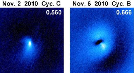
Figure 7: Comparison of the transient structures in the CN coma on November 2 (Cycle C) and November 6 (Cycle B). Each panel presents the result of subtraction of the reference residual image (November 5) from the actual residual frame. Phases are displayed in the upper-right corners. Orientation and image scale are identical as in Fig. 1.

Figure 7 presents one example of the subtraction result for November 2 and one for November 6. The striking difference is easily visible. While on November 2 a bright jet directed southward was present, the November 6 image shows an elliptical envelope with a pair of bright spots. The jet visible on the first night was brightening with time and then diminished a bit. It contributed to the CN signal in our aperture, increasing it to the highest level observed during the whole run. The night of November 6 (Cycle B) provides us with the CN pattern that closely resembles the CN structure from November 4 (Cycle C) but is about two times smaller. The position angles of the bright spots from November 6 correlate very well with the position angles of the similar features from November 4. Discrepancies are 1° and 10° for structures A and B respectively, but anyway of the order of the error bars. The reason for this similarity is that we observe different evolution stages (phase difference $\sim$0.4) of the same structure which appears periodically every three precession cycles. More precisely, these are the similarities between two different Cycles B: one on November 6 and the other one preceding Cycle C on November 4. We note, however, that both Cycles B exhibited different profiles of the CN features and dissimilar evolution. Moreover, the CN structures visible on November 4 moved slowly (0.14 km s^-1 for part A and 0.28 km s^-1 for feature B), whereas the structures for November 6 expanded much faster (0.66 km s^-1 and 0.43 km s^-1 for structures A and B respectively). Taking into account the very stable radial evolution of the corkscrew structure on November 6 (especially its south-west part), not exhibiting the spiral or wavy pattern, we suspect that this phenomenon was created by a fan with a relatively large opening angle enclosing the Earthward direction. The fan was rotating as the nucleus was rotating about the precession axis which was enclosed in this fan as well. The source of such a flat feature having a large extent could be a properly oriented deep trench. Such topographic element could lie along the border between the ”waist“ region and one of the nucleus lobes.

To explain the unexpected rise of the expansion velocity for this corkscrew pattern compared to the slowly moving CN features on the previous nights we need a significantly different influence of the projection effect. If our interpretation of the corkscrew structure is true, the on-sky projection did not affect markedly the observed velocity on November 6 and hence it should be close to the real expansion velocity of the gas. This possibility implies that the opening angle of the fan producing the corkscrew structure was indeed huge compared to the opening angle of the CN ejection on November 4.

Comet 103P presents evident dissimilarities in the CN transient patterns and their on-sky kinematics (see Section 4) for successive Cycles A, B and C. Similar variations in the line-of-sight kinematcs of HCN, the most likely progenitor of CN, have been reported by Drahus et al. (drahus12 (2012)). The most natural explanation seems to be the one with a typical gas flow velocity of the order of 1 km s^-1 and variation in the direction of the dominant gas ejection which changes markedly from one cycle to another. The precession-roll scenario, proposed by A’Hearn et al. (ahearn11 (2011)), appears to provide a plausible explanation and relates well to the extraordinary spin-down of the comet’s nucleus resulting most probably from the jet effect, which can also enforce the excited mode of rotation (e.g. Gutiérrez et al. gutierrez03 (2003)). In such a case, one and the same active vent (e.g. the region recorded by EPOXI on the smaller tip of the nucleus) can eject matter in different directions and also other vents can be insolated during some or all of the precession cycles.

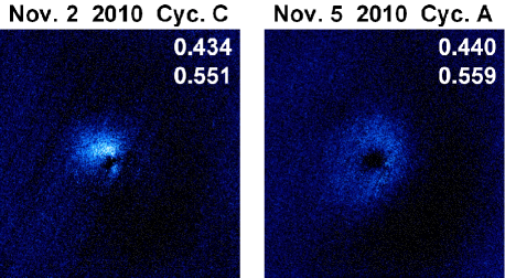
Figure 8: Evolution of the central CN shell observed on November 2 (Cycle C) and November 5 (Cycle A). The behaviour in time is displayed by the result of subtraction of the earlier exposure from the later one. Precession phases are shown in the upper right corners. Orientation and image scale are the same as in Fig. 1.

Since the three consecutive precession cycles produced different coma structures, it is interesting to examine if these structures also evolved differently. Analysing video clip Animation2 we conclude that the expansion of the central shell observed on November 2 (Cycle C) varied substantially compared to the behaviours observed on November 5 (Cycle A) and 6 (Cycle B). The former case presents an expanding, spiral-like structure in the northern part of the central feature. To ensure that this is not an artefact produced by our version of the ring-masking procedure (used to generate video clip Animation2) we verified the result using a simple algebra for the residual images. To enhance the signal-to-noise ratio we stacked image #1 with #2, and #4 with #5 from November 2, and also #4 with #5, and #8 with #9 from November 5. Consequently, for each of the two nights we obtained a pair of images with the time differences equal to 2.1 and 2.2 hours for November 2 and November 5, respectively. Then we subtracted the earlier image from the later one in each pair (all the frames were carefully normalized before). Such differential images (Fig. 8) clearly show the evolution of the central CN patterns as the difference of signals correlates with time increment, i.e. higher values imply later stages of evolution. The results confirm our previous findings. On November 2 we observed the rotating spiral-like structure produced by a clockwise nucleus precession as projected on the sky. This case resembles the well developed spirals reported for 103P in September-October (see e.g. Samarasinha et al. samarasinha11 (2011)). The ellipsoidal shell observed on November 5 expanded highly symmetrically. Such a behavior is fully consistent with the scenario of gas ejection into a wide cone enclosing the Earthward direction. Prolateness of this envelope is controlled by the nucleus precession that changes the orientation of the active tip during the insolation phase producing the typical spiral which is visible almost completely edge-on on this date. We observe a similar situation on November 6.

The dissimilarity in the evolution of the central CN shell noticed between Cycles C and A may be caused by the roll about the longest axis of the nucleus (A’Hearn et al. ahearn11 (2011)). It is sufficient that the active vent, which occupies the smaller tip of the nucleus, is shifted off the roll axis.

7 Orientation of the nucleus rotation axis

We determine the orientation of the rotation axis assuming for simplicity that the nucleus was a SAM rotator with the spin axis which is close to the precession axis. We noticed in Section 6 that the corkscrew structure (especially its south-west part) visible on November 6 expanded strictly radially and the position angles of its expansion direction correlate with the traces of the corkscrew pattern from November 4. Hence, for different precession cycles there is one distinguished direction, which we attribute to the on-sky projection of the rotation axis of 103P. If so, the south-west section of the corkscrew structure was created by a circumpolar gas jet. As the on-sky velocity of this pattern was relatively high, it expanded in a direction far from the line of sight, forming a conical structure consistent with our observations. Thus, we have assumed that the symetry axis of the south-west part of the corkscrew structure corresponds with the on-sky projection of the nucleus rotation axis.

In the next step we used the in situ determination of an instantaneous orientation of the longest axis of 103P’s nucleus during the EPOXI flyby (A’Hearn et al. ahearn11 (2011)), which we consider as representing the shortest axis of inertia. It is obvious that the rotation axis has to lie in the plane perpendicular to this axis. Figure 9 presents this situation. On the other hand, the on-sky projection of the rotation axis should coincide with the direction of the south-west part of the corkscrew pattern. Combining both restrictions we find the orientation of the north rotation pole (the sense of spinning is determined in Section 6) as RA=122° and Dec=+16° (epoch J2000.0).

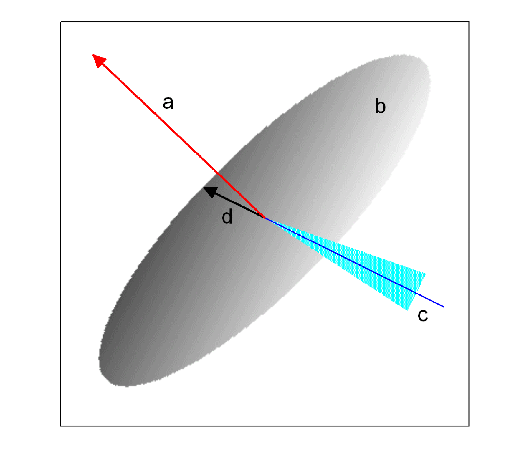
Figure 9: Sketch illustrating how the orientation of the rotation axis was determined. This is an on-sky projection with orientation like in Fig. 1. Circular plane b is perpendicular to vector a, which represents the direction of the shortest axis of inertia of the comet’s nucleus. Line segment c shows the on-sky direction of the axis of the corkscrew pattern. Angular momentum vector d shows our solution. It should be located at plane b, and its on-sky projection should coincide with line segment c.

The error of our determinantion is dominated by the validity level of our assumptions which is very difficult to estimate. If the assumptions were strictly satisfied, the obtained circular error would be 2° which we computed by propagating the uncertainty of the position angle of the south-west part of the corkscrew structure and the error of the orientation of the longest nucleus axis (A’Hearn et al. ahearn11 (2011)).

A’Hearn et al. (ahearn11 (2011)) found the direction of the total angular momentum (close to the precession axis) equal to RA=17$\pm$11° and Dec=+47$\pm$2°. Radar Doppler imaging (Harmon et al. 2011b ) gave the result RA=332° and Dec=+20°. Analysis of the CN coma structures made by Knight & Schleicher (knight11 (2011)) shows the axis direction of RA=257° and Dec=+67° with the uncertainty of 15°, and Samarasinha et al. (samarasinha11 (2011)) obtained RA=345°, Dec=$-$15° with a 20° precision. Although, it is hard to obtain a coherent picture from these results, all the solutions (including ours) are preliminary at this stage.

8 Comparison of CN and HCN

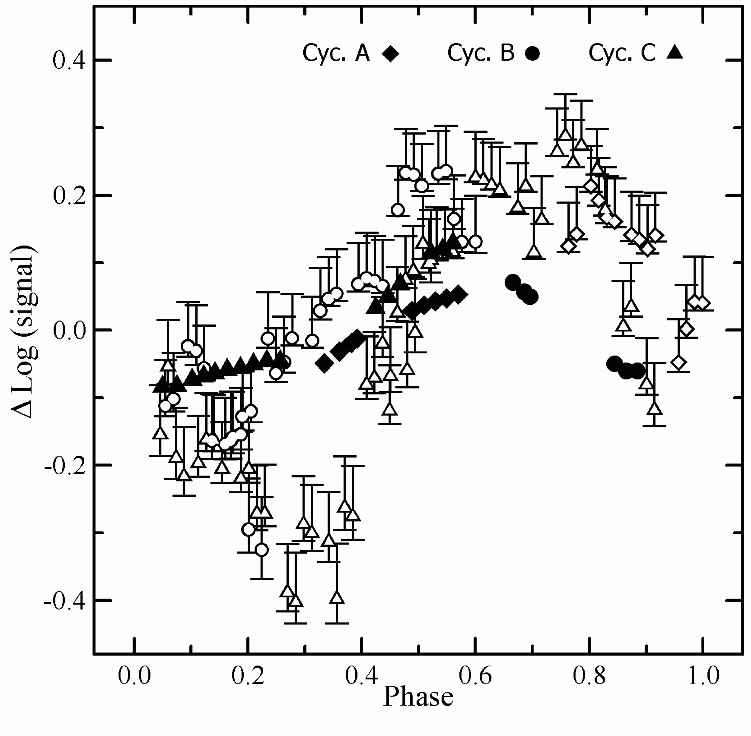
Figure 10: Comparison between the molecular light curves of CN (see text) and HCN (from Drahus et al. drahus11 (2011)). The HCN signal is represented by the line area measured in the beam of 8.8-arcsec FWHM. The light curves are calculated with respect to the mean levels, and phased according to the 18.32 h period. The filled symbols are used for CN and the open symbols for HCN, while the symbol shape indicates the three-cycle component. The error bars for CN are of the order of the symbol size and have been omitted.

Since we noticed the exceptional coincidence of the rotation periods from the HCN and CN data (cf. Section 5), we also examined the correlation between both molecules, comparing the variability in the relative photometry of CN (Section 5) with a series of the HCN main-beam brightness temperatures from IRAM 30-m (the latter being a part of the observing material obtained by Drahus et al. drahus11 (2011); drahus12 (2012)). Both the CN photometry and the HCN data selected for comparison were collected around the same time and partly simultaneously. Figure 10 presents this comparison, where the data are phased in the same way as before (cf. Sections 3 and 5), and identically for all practical purposes with Drahus et al. (drahus11 (2011)).

It should be born in mind that HCN was monitored with the beam size three times smaller than the aperture used for our CN photometry. Hence, the CN variability can be phase-delayed as compared with HCN. Such an aperture effect was discussed in Section 5 and found negligible. The markedly smaller amplitude of variability for CN may result from smoothing introduced by the finite lifetime of the CN parent ($\sim$10⁴ s for HCN). In general, both light curves correlate quite well in the active phases and much worse during the quiescent periods. Perhaps CN in 103P originates from two different sources, each behaving differently. One source could be related to insolated active vents and the other one to different parts of the nucleus surface or to a volume source surrounding the nucleus, such as e.g. the ”snowflakes“ detected by EPOXI (A’Hearn et al. ahearn11 (2011)). To look deeper into the correlation between HCN and CN a non-steady-state model of the HCN-CN coma has to be build, which is a subject of our ongoing work.

9 Conclusions

1. Image processing of the CN and C₃ frames revealed transient structures in the gas coma of 103P. Both radicals formed very similar features at close time moments. CN and C₃ photometry shows general consistence. We conclude that the progenitors of CN and C₃ were emitted from the same regions of the nucleus, which implies homogeneity of the CN and C₃ parents.

2. The CN signal varied with a period of 18.32$\pm$0.30 h at the epoch of our observations (UT 2010 Nov. 5.0835), the same as was measured for HCN around the same time. The variability of HCN correlates with the behaviour of CN suggesting that HCN was a major donor of CN.

3. The CN structures expanded with projected velocities between 0.1 and 0.3 km s^-1, except for November 6, when the velocity increased up to 0.66 km s^-1 in the south-west part of the corkscrew pattern.

4. The CN shells, appearing in the central part of the coma at the phases of boosted CN production, present a high level of cross-correlation. They were most probably generated by periodic insolation of the smaller tip of the nucleus (active at the EPOXI encounter). The CN profiles at the consecutive Cycles A, B and C differed markedly. A modest CN boosting was observed during Cycle A (November 5), a corkscrew pattern was present during Cycle B (November 6), and a southern jet was visible at Cycle C (November 2). They suggest that for different cycles different nucleus parts, carrying different vents, were exposed to the solar radiation and active.

5. Although the corkscrew structure seems to appear every three precession cycles, the situation did not repeat strictly (different profiles and kinematics).

6. Combining the results of our image analysis with the instantaneous nucleus orientation from EPOXI and assuming the principal-axis rotation mode we obtained the orientation of the spin axis equal to RA=122° and Dec=+16° (epoch J2000.0).

Appendix A Image cleaning procedure

With the aim to remove Cosmic Ray Hits (CRH) and stellar profiles elongated by non-sidereal tracking we grouped consecutive images in pairs and compared the first frame with the second frame in each pair. We took advantage of the statistical independence of CRH, and the fact that in two consecutive frames a given stellar trail occupies separable regions (the 40-s CCD readout time corresponds to 3 arcsec of comet’s motion). We subtracted and averaged images in pairs, obtaining two series of images: one with differential frames and other one with mean frames. For each differential image we correlated its noise statistics with the mean signal in the corresponding averaged frame. Using the dependence between noise level and mean signal it is possible, for a given pixel, to estimate the dispersion of signal in the differential frame. When the pixel value in the differential image was higher than $K\sigma$ (i.e. a factor of $K$ above the local noise) we flagged it in an auxiliary binary mask frame. As the stellar patterns in the auxiliary mask frames contain regions with disconnected pixels (external envelopes of bright stars and whole patterns for stars at the noise limit) we produced compact patterns improving pixel connectivity. We used the closing-like procedure based on the local surface density of the flagged pixels. For a given pixel, the density was probed in a small circle surrounding this pixel and compared with the limiting value. This value was determined using the trial-and-error procedure. Above this limit the pixel was kept flagged and vice versa. This stage of image processing was completed by synthesizing clean stacks. In the regions where no CRHs or stellar trails were detected, the mean values from both frames were taken. Otherwise, the values from the image with no detection were accepted. As the comet was observed in relatively dense stellar fields, the profiles of different stars occasionally overlapped in the images from one pair. In such situations the stellar trails were masked and filled using interpolation. By stacking two consecutive images we increased the signal-to-noise ratio except for the regions occupied by the stellar profiles or CRHs. We note that in rare cases one and the same frame was used to create two consecutive pairs. Obviously, such pairs are not independent, but let us use the entire nightly material, even if the number of single images is odd. Figure 11 presents one example of how our cleaning procedure is able to remove unwanted objects from the comet image.

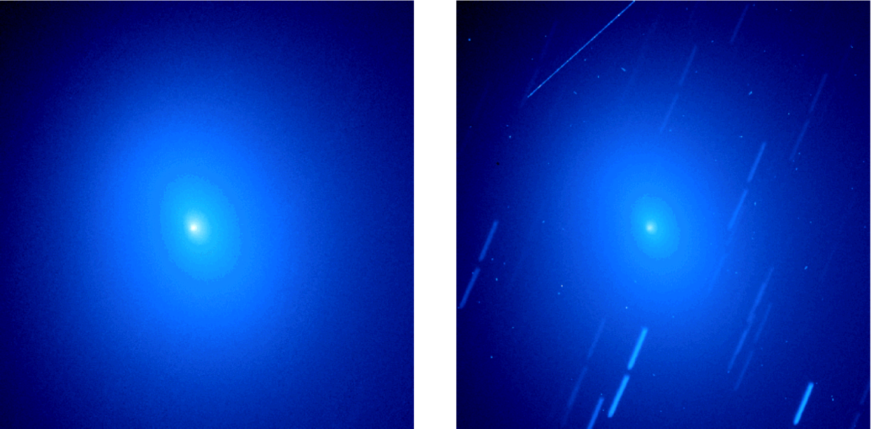
Figure 11: Result of removal of CRHs and stellar profiles by the cleaning procedure (left pannel). For comparison, the right panel shows the result of simple stacking of the same two frames. Date of observation is UT 2010 Nov. 7.1375. The field of view is 6.4 arcmin. North is up and east is to the left.