The symplectic-$N$ t-J model and s_± superconductors

Abstract

The possible discovery of $s_{\pm}$ superconducting gaps in the moderately correlated iron-based superconductors has raised the question of how to properly treat $s_{\pm}$ gaps in strongly correlated superconductors. Unlike the d-wave cuprates, the Coulomb repulsion does not vanish by symmetry, and a careful treatment is essential. Thus far, only the weak correlation approaches have included this Coulomb pseudopotential, so here we introduce a symplectic $N$ treatment of the $t-J$ model that incorporates the strong Coulomb repulsion through the complete elimination of on-site pairing. Through a proper extension of time-reversal symmetry to the large $N$ limit, symplectic-$N$ is the first superconducting large $N$ solution of the $t-J$ model. For d-wave superconductors, the previous uncontrolled mean field solutions are reproduced, while for $s_{\pm}$ superconductors, the $SU(2)$ constraint enforcing single occupancy acts as a pair chemical potential adjusting the location of the gap nodes. This adjustment can capture the wide variety of gaps proposed for the iron based superconductors: line and point nodes, as well as two different, but related full gaps on different Fermi surfaces.

I Introduction

The new family of iron-based superconductorshosano08 has expanded the study of high temperature superconductors from the single band, d-wave cuprate superconductors to include multi-band superconductors with full gaps. Experimentallynn09 and numericalsi08 ; haule08 ; kutepov10 work suggest a range of correlation strengths between different materials. From the theoretical point of view, weak and strong correlation approaches converge on many of the major features: most importantly, the predominantly $s_{\pm}$ structure of the superconducting gapmazin08 ; chubukov08 ; si08 ; seo08 ; parish08 ; maier09 ; wang09 ; sknepnek09 ; yao09 ; hu11 ; hirschfeld11 . The real materials are likely in the regime of moderate correlations where both approaches are useful. Unlike the d-wave cuprates, where the strong Coulomb repulsion is eliminated by symmetry, these multi-band $s_{\pm}$ superconductors require a careful treatment of the Coulomb pseudopotentialmorel62 . While this has been incorporated into weak coupling approacheschubukov08 ; maier09 ; sknepnek09 ; mazin09 , it has yet to be included in strong correlation treatments based on the $t-J$ model. With this in mind, we introduce the symplectic-$N$ $t-J$ model. The use of a large $N$ limit based on the symplectic group, $SP(N)$ allows a proper treatment of time-reversal in the large-$N$ limitflint08 ; flint09 ; flint11 , making this the first superconducting large $N$ treatment of the $t-J$ model. Symplectic-$N$ also replaces the usual $U(1)$ constraint of single-occupancy with a $SU(2)$ constraint that strictly eliminates on-site pairingflint11 . This $SU(2)$ constraint is essential to the treatment of $s_{\pm}$ superconductors, where it acts as a pair chemical potential, adjusting the gap nodes to eliminate the Coulomb repulsion.

This paper is intended as an introduction to the symplectic-$N$ $t-J$ model, illustrating the importance of the additional constraint with the example of $s_{\pm}$ superconductors, and showing how this model contains a range of gap behaviors reproducing different iron-based materials. We begin by reviewing the Coulomb pseudopotential in section II and demonstrate the lack of superconductivity in the $SU(N)$ $t-J$ model corresponding to the usual slave boson mean field theory. In section III, we introduce symplectic Hubbard operators, which allow us to develop a superconducting large-$N$ treatment of the $t-J$ model. We demonstrate this mean field theory on several examples in section IV, before discussing the range of possible future directions in V.

II The Coulomb pseudopotential and the $t-J$ model

On-site pairing is disfavored by the Coulomb pseudopotential, which will cost a bare energy, $UN(0)$, the average of the Coulomb repulsion, $V({\bf{r}}_{i}-{\bf{r}}_{j})=e^{2}/|{\bf{r}}_{i}-{\bf{r}}_{j}|$ over the Fermi sea. However, in the weak coupling limit, where we assume the pairing is mediated by the exchange of a boson with characteristic frequency $\omega_{B}$, the time scale of the pairing, $\omega_{B}$ is much longer than that of the Coulomb repulsion. In other words, while the effective electron-electron interaction is attractive, it is also retarded, meaning the electrons like to be in the same place, but at different times, while the Coulomb repulsion is a nearly instantaneous repulsion of two electrons at the same place and time. The Coulomb pseudopotential is therefore renormalizedmorel62 ,

$$\mu^{*}=\frac{N(0)U}{1+N(0)U\log\frac{E_{F}}{\omega_{B}}}$$ (1)

to weak coupling. If $T_{c}\propto\omega_{B}\exp(-1/\lambda)$, the attractive interaction is replaced by $\lambda\rightarrow\lambda-\mu^{*}$, which reduces $T_{c}$ slightly at weak coupling, but does not destroy superconductivity. In BCS superconductivity, the bosons exchanged are phonons, and the Debye frequency, $\omega_{D}\ll E_{F}$. However, in more strongly correlated superconductors, the two time scales are of the same order, and the Coulomb pseudopotential can drastically affect the superconductivity. Strongly correlated examples, like the cuprate and heavy fermion superconductors, avoid this problem by developing a d-wave gap, where the pairing with a positive gap is exactly cancelled out by that with a negative gap, as guaranteed by the d-wave symmetry. This choice of gap neutralizes the Coulomb pseudopotential. However, the iron-based superconductors are widely believed to have an $s_{\pm}$ gap, where the amount of cancellation between positive and negative gap regions is not protected by symmetry, and depends strongly on the Fermi surfaces. When this cancellation is incomplete, $\mu^{*}$ reduces $T_{c}$ and it is extremely important to consider this effect when mapping out the phase diagram, as it affects the relative stability of s- and d-wave gaps. These effects have been incorporated in the weakly correlated solutionschubukov08 ; maier09 ; sknepnek09 ; mazin09 , but not yet in the strongly correlated approaches.

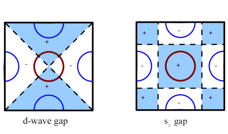
Figure 1: (Left) In the d-wave gap, the cancellation of the superconducting order parameter over the Fermi surface is guaranteed by symmetry, as the positive (blue) regions will exactly cancel the negative (white) regions. (Right) However, in the $s_{\pm}$ superconducting gap, the amount of cancellation is extremely sensitive to the Fermi surface.

Here, we take the strongly correlated limit, $U\rightarrow\infty$ to eliminate double occupancy, which corresponds to taking $\mu^{*}\rightarrow\infty$. The Heisenberg model describes the insulating half-filled limit of the $t-J$ model, but generally holes ($n<1$) or electrons ($n>1$) will hop around in an antiferromagnetic background. Doubly occupied states must be avoided, and the hopping is not that of free electrons. Rather, it is projected hopping, described by the $t-J$ modelspalek77 ; anderson87 ,

$$H=-\sum_{ij}t_{ij}\left[X_{\sigma 0}(i)X_{0\sigma}(j)+\mathrm{H.c.}\right]+\sum_{ij}J_{ij}\vec{S}_{i}\cdot\vec{S}_{j}.$$ (2)

The Hubbard operators, $X_{ab}=|a\rangle\langle b|$, where $|a\rangle=|0\rangle,|\sigma\rangle$ ensure that only empty sites, or holes can hop (or for $n>1$ that electrons can only hop from doubly occupied sites to singly occupied sites). Here, $X_{\sigma 0}$ are projected hopping operators

Exact solutions of the $t-J$ model are unavailable, and the typical approach is to write down a mean field solution using the slave boson approachkotliarliu88 ; wenlee96 ; lee06 , which divides the electron into charged, but spinless holons and neutral spinons. The most common choice is the $U(1)$ slave boson representationcoleman83 ,

$$X_{\sigma 0}=f^{\dagger}_{\sigma}b,$$ (3)

so-called because it is invariant under $U(1)$ gauge transformations. However, mean field solutions do not necessarily satisfy all the conditions on the full model, and may not maintain the $\mu^{*}\rightarrow\infty$ limit. Large $N$ approaches generate mean-field solutions by extending the $SU(2)$ $t-J$ model to some larger group. When developing a large $N$ treatment of the hopping term, one must take care that the two terms are consistent, or in other words, that the charge fluctuations described by the $t$ term generate the spin fluctuations in the Heisenberg term. The algebra of these operators, given by

$$\{X_{\alpha 0},X_{0\beta}\}=f^{\dagger}_{\alpha}f_{\beta}+b^{\dagger}b\delta_{\alpha\beta}.$$ (4)

extends the algebra of Hubbard operators from $SU(2)$ to $SU(N)$, and we see that two charge fluctuations in sequence give rise to a spin fluctuation described by the $SU(N)$ spin operator $X_{\alpha\beta}=f^{\dagger}_{\alpha}f_{\beta}$.

The large $N$ limit of the full $SU(N)$ $t-J$ model is:

$$H=-\!\sum_{\langle ij\rangle}\!\frac{t_{ij}}{N}\!f^{\dagger}_{i\alpha}b_{i}b_{j}^{\dagger}f_{j\alpha}+\!\sum_{ij}\!\frac{J_{ij}}{N}\!\left(f^{\dagger}_{i\alpha}f_{j\alpha}\!\right)\!\left(f^{\dagger}_{j\beta}f_{i\beta}\!\right)\!.$$ (5)

Decoupling the $J$ term yields a dispersion for the spinons, but not pairingaffleckmarston88 . There is no superconductivity in this large $N$ limit.

III The symplectic-$N$ $t-J$ model

A superconducting large $N$ limit requires a proper definition of time-reversal, as Cooper pairs can only form between time-reversed pairs of electrons. The inversion of spins under time-reversal is equivalent to symplectic symmetry, and the only way to preserve time-reversal in the large $N$ limit is to use symplectic spinsflint08 ; flint09 ,

$$S_{\alpha\beta}=f^{\dagger}_{\alpha}f_{\beta}-\tilde{\alpha}\tilde{\beta}f^{\dagger}_{-\beta}f_{-\alpha},$$ (6)

where $\alpha$ ranges from $-N/2$ to $N/2$ and $\tilde{\alpha}=\mathrm{sgn}(\alpha)$. Here we use the fermionic representation because we are interested in the doped spin liquid states that become superconductors. Introducing doping means introducing a small number of mobile empty states. When an electron hops on and off a site, it can flip the spin of the site. Mathematically, this implies that the anticommutator of two Hubbard operators generates a spin operator. In a symplectic-$N$ generalization of the t-J model, anticommuting two such Hubbard operators must generate a symplectic spin, satisfying the relations:

$$\left\{X_{\alpha 0},X_{0\beta}\right\} = X_{\alpha\beta}+X_{00}\delta_{\alpha\beta}$$

$$= S_{\alpha\beta}+\left(X_{00}+\frac{X_{\gamma\gamma}}{N}\right)\delta_{\alpha,\beta},$$

where the last equality follows from the traceless definition of the symplectic spin operator, $S_{\alpha\beta}=X_{\alpha\beta}-\frac{X_{\gamma\gamma}}{N}\delta_{\alpha\beta}$. When we represent the Hubbard operators with slave bosons, the symplectic projected creation operators take the following formflint11 ,

$$X_{\alpha 0}=f^{\dagger}_{\sigma}b+\tilde{\sigma}f_{-\sigma}a,$$ (8)

so that the other two Hubbard operators take the form

$$X_{\alpha\beta} = S_{\alpha\beta}+\delta_{\alpha\beta}$$ (9)

$$X_{00} = b^{\dagger}b+a^{\dagger}a.$$ (10)

This double slave boson form for Hubbard operators was derived by Wen and Leewenlee96 as a way of extending the local $SU(2)$ symmetry of spin to include charge fluctuations. In our approach the $SU(2)$ symmetry appears as a consequence of the time-inversion properties of symplectic spins for all even $N$, which permits us to carry out a large $N$ expansion. The Nambu notation, $B^{\dagger}=(b^{\dagger},a^{\dagger})$ and $\tilde{f}^{\dagger}=(f^{\dagger}_{\alpha},\tilde{\alpha}f_{-\alpha})$ simplifies the expressions, as $X_{\alpha 0}=\tilde{f}^{\dagger}_{\alpha}B$ and the hopping term of symplectic-$N$ $t-J$ model can be written,

$$H\!\! = \!\!\!-\!\sum_{ij}\!\frac{t_{ij}}{N}\!\!\left[\!\left(f^{\dagger}_{i\alpha}b_{i}+\tilde{\alpha}f_{i-\alpha}a_{i}\right)\!\!\left(f_{j\alpha}b_{j}^{\dagger}+\tilde{\alpha}f^{\dagger}_{j-\alpha}a_{j}^{\dagger}\right)\!+\!\mathrm{H.c.}\!\right]$$ (11)

$$= \!\!\!-\!\sum_{ij}\!\frac{t_{ij}}{N}\left(\tilde{f}^{\dagger}_{i\alpha}B_{i}B_{j}^{\dagger}\tilde{f}_{j\alpha}+\mathrm{H.c.}\right)$$ (12)

Restricting the spin and charge fluctuations to the physical subspace requires that we fix the Casimir of the Hubbard operatorshopkinson ,

$${\cal C}=\vec{S}_{j}^{2}+\left[X_{0\alpha},X_{\alpha 0}\right]-(X_{00}+1)^{2},$$ (13)

where $\vec{S}_{j}^{2}=\frac{1}{2}\sum_{\alpha\beta}S_{\alpha\beta}(j)S_{\beta\alpha}(j)$. A detailed calculation (see Appendix) shows that

$${\cal C}=(N/2)^{2}-1-\vec{\Psi}_{j}^{2},$$ (14)

where $\vec{\Psi}\equiv(\Psi^{\dagger},\Psi,\Psi_{3})$ is given by

$$\Psi_{3} = n_{f}+n_{b}-n_{a}-\frac{N}{2}$$ (15)

$$\Psi^{\dagger} = \sum_{\alpha>0}f^{\dagger}_{\alpha}f^{\dagger}_{-\alpha}+b^{\dagger}a$$ (16)

$$\Psi = \sum_{\alpha>0}f_{-\alpha}f_{\alpha}+a^{\dagger}b.$$ (17)

In the infinite-$U$ limit, the Casimir, $\mathcal{C}$ is set to its maximal value, and we obtain the constraint $\vec{\Psi_{j}}=0$. Writing out the condition that $\vec{\Psi_{j}}$ vanishes, we obtain

$$b_{j}^{\dagger}b_{j}-a_{j}^{\dagger}a_{j}+f^{\dagger}_{j\alpha}f_{j\alpha}=N/2$$ (18)

$$b_{j}^{\dagger}a_{j}+\sum_{\alpha>0}\tilde{\alpha}f^{\dagger}_{j\alpha}f^{\dagger}_{j-\alpha}=0$$ (19)

$$a_{j}^{\dagger}b_{j}+\tilde{\alpha}f_{j-\alpha}f_{j\alpha}=0.$$ (20)

The first equation imposes the constraint on no double occupancy. The second terms play the role of a Coulomb pair pseudo-potential, forcing the net s-wave wave pair amplitude to be zero when superconductivity develops. Under the occupancy constraint, there is only a single physical empty state, which is

$$|0\rangle=\left(b^{\dagger}+a^{\dagger}\tilde{\alpha}f^{\dagger}_{-\alpha}f^{\dagger}_{\alpha}\right)|\Omega\rangle,$$ (21)

for $N=2$. The physical interpretation of these terms becomes clearer if we pick a particular gauge. Since we only have two flavors of bosons and N flavors of fermions, the only way the bosons contribute in the large N limit is by condensing. As the bosons are condensed at all temperatures, Fermi liquids and superconductors are the only possible states; while this situation is clearly unphysical, and will be resolved with 1/N corrections, it allows us to fix the gauge in a particularly simple way by setting $a=0$ and condensing only the $b$ bosons, $b^{2}=Nx/2$ because the bosons carry all the charge in the system. The factor of $N/2$ makes the doping extensive in $N$. The constraint simplifies to,

$$f^{\dagger}_{j\alpha}f_{j\alpha} = \frac{N(1-x)}{2}$$ (22)

$$\tilde{\alpha}f^{\dagger}_{j\alpha}f^{\dagger}_{j-\alpha} = 0$$ (23)

$$\tilde{\alpha}f_{j-\alpha}f_{j\alpha} = 0,$$ (24)

In a mean field theory, these three constraints are enforced by a trio of Lagrange multipliers $\vec{\lambda}=(\lambda_{+},\lambda_{-},\lambda_{3})$ in a constraint term that takes the form

$$H_{C}=\sum_{j}\lambda_{3}\left[f^{\dagger}_{j\alpha}f_{j\alpha}-\frac{N(1-x)}{2}\right]+\lambda_{+}(\tilde{\alpha}f^{\dagger}_{j\alpha}f^{\dagger}_{j-\alpha})+{\rm H.c}$$ (25)

The first constraint is clearly recognizable as imposing Luttinger’s theorem. This term is present in the conventional $U(1)$ slave boson approachkotliarliu88 . The second terms impose severe constraints on the pair wavefunction when superconductivity develops, implementing the infinite Coulomb pseudopotential. For d-wave superconductors like the cuprates, which have been the main focus of previous $t-J$ model studies, these constraints are satisfied automatically, and at the mean-field level, there is no difference between the symplectic-$N$ limit and many of the previously considered uncontrolled mean field theorieskotliarliu88 ; wenlee96 ; vojta99 . However, for $s_{\pm}$ pairing, these additional constraints enforce the Coulomb pseudopotential, $\mu^{*}$ and have a large effect on the stability of $s_{\pm}$ superconductivity.

Once the bosons are condensed, and the Heisenberg term decoupled, the spinon Hamiltonian is quadratic,

$$H=\!\sum_{ij}\!\tilde{f}^{\dagger}_{i}\!\left[-\frac{xt_{ij}}{2}\tau_{3}+U_{ij}\!\right]\!\tilde{f}_{j}+\frac{N\!\left[|\Delta_{ij}|^{2}+|\chi_{ij}|^{2}\right]}{J_{ij}},$$ (26)

where we have introduced the $SU(2)$ matrix notation,

$$U_{ij}=\left[\!\begin{matrix}-\chi_{ij}&\Delta_{ij}\cr\bar{\Delta}_{ij}&\bar{\chi}_{ij}\end{matrix}\!\right].$$ (27)

$\chi_{ij}$ generates a dispersion for the spinons, while $\Delta_{ij}$ pairs them. The full Hamiltonian is given by $H+H_{C}$. The physical electron, $c^{\dagger}\sim\langle b\rangle f^{\dagger}+\langle a\rangle f$ will either hop coherently, forming a Fermi liquid when $\Delta$ is zero, or will superconduct when $\Delta$ is nonzero. The mean field phase diagram is obtained by minimizing the free energy with respect to these mean field parameters, $\chi_{ij}$ and $\Delta_{ij}$,

$$\chi_{ij} = \frac{J_{ij}}{N}\langle f^{\dagger}_{i\alpha}f_{j\alpha}\rangle$$ (28)

$$\Delta_{ij} = \frac{J_{ij}}{N}\langle\tilde{\alpha}f^{\dagger}_{i\alpha}f^{\dagger}_{j-\alpha}\rangle,$$ (29)

and enforcing the constraint on average, $\langle\sum_{j}f^{\dagger}_{j\alpha}f_{j\alpha}\rangle=\frac{N(1-x)}{2}$ and $\langle\sum_{j}\tilde{\alpha}f^{\dagger}_{j\alpha}f^{\dagger}_{j-\alpha}\rangle=0$, where $\langle\cdots\rangle$ is the thermal expectation value.

The $J_{1}-J_{2}$ model will have two sets of bond variables, $\chi_{\eta}$ and $\Delta_{\eta}$, where $\eta$ indicates a link, $(ij)$. We assume that $\chi_{1}$ and $\chi_{2}$ are uniform, and allow $\Delta_{1}$ and $\Delta_{2}$ to be either s-wave or d-wave. When these order parameters are Fourier transformed, we find $\chi_{\bf{k}}=\chi_{1}\gamma_{1{\bf{k}}}+\chi_{2}\gamma_{2{\bf{k}}}\equiv 2\chi_{1}(c_{x}+c_{y})+4\chi_{2}c_{x}c_{y}$ and $\Delta_{\bf{k}}=\sum_{\eta}\Delta_{\eta}\delta_{\eta{\bf{k}}}$ is a combination of s-wave and d-wave pairing on the nearest and next nearest neighbor links,

$$\mathrm{extended}\;s 2\Delta_{1s}(c_{x}+c_{y})$$ (30)

$$d_{x^{2}-y^{2}} 2\Delta_{1d}(c_{x}-c_{y})$$ (31)

$$s_{\pm} 2\Delta_{2s}(c_{x+y}+c_{x-y})=4\Delta_{2s}c_{x}c_{y}$$ (32)

$$d_{xy} 2\Delta_{2d}(c_{x+y}-c_{x-y})=-4\Delta_{2d}s_{x}s_{y}$$ (33)

and we define $c_{\eta}=\cos k_{\eta}a$, $s_{\eta}=\sin k_{\eta}a$. The full Hamiltonian (including the constraint) has the form,

$$H = \sum_{\bf{k}}\tilde{f}^{\dagger}_{\bf{k}}\left(-\frac{x\epsilon_{\bf{k}}}{2}+U_{\bf{k}}+\lambda_{3}\tau_{3}+\lambda_{1}\tau_{1}\right)\tilde{f}_{\bf{k}}$$ (35)

$$+\mathcal{N}_{s}\sum_{\eta}\frac{N}{J_{\eta}}\left(|\Delta_{\eta}|^{2}+|\chi_{\eta}|^{2}\right)-\frac{N\mathcal{N}_{s}x\lambda_{3}}{2}$$

where $\epsilon_{k}$ is the Fourier transform of $t_{ij}$, $U_{\bf{k}}$ is the Fourier transform of $U_{ij}$ and $\lambda_{1}=\frac{1}{2}(\lambda_{+}+\lambda_{-})$. ($\lambda_{2}$ is unnecessary if $\Delta$ is real). This Hamiltonian can be diagonalized, and the spinons integrated out to yield the free energy,

$$F = -2NT\sum_{{\bf{k}}}\log 2\cosh\frac{\beta\omega_{{\bf{k}}}}{2}$$ (37)

$$+\mathcal{N}_{s}\sum_{\eta}\frac{4N}{J_{\eta}}\left(|\Delta_{\eta}|^{2}+|\chi_{\eta}|^{2}\right)-\frac{N\mathcal{N}_{s}x\lambda_{3}}{2},$$

where $\omega_{\bf{k}}=\sqrt{\alpha_{\bf{k}}^{2}+\beta_{\bf{k}}^{2}}$, $\alpha_{\bf{k}}=\lambda_{3}-\frac{x\epsilon_{\bf{k}}}{2}+\chi_{\bf{k}},$ and $\beta_{\bf{k}}=\lambda_{1}+\Delta_{\bf{k}}$. Minimizing this free energy leads to the four mean field equations,

$$\partial F/\partial\chi_{\eta} = \int_{\bf{k}}\frac{\tanh\frac{\beta\omega_{\bf{k}}}{2}}{2\omega_{\bf{k}}}\alpha_{\bf{k}}\gamma_{\eta{\bf{k}}}-\frac{4}{J_{\eta}}=0$$ (38)

$$\partial F/\partial\Delta_{\eta} = \int_{\bf{k}}\frac{\tanh\frac{\beta\omega_{\bf{k}}}{2}}{2\omega_{\bf{k}}}\beta_{\bf{k}}\delta_{\eta{\bf{k}}}-\frac{4}{J_{\eta}}=0$$ (39)

$$\partial F/\partial\lambda_{3} = \int_{\bf{k}}\frac{\tanh\frac{\beta\omega_{\bf{k}}}{2}}{2\omega_{\bf{k}}}\alpha_{\bf{k}}-x/2=0$$ (40)

$$\partial F/\partial\lambda_{1} = \int_{\bf{k}}\frac{\tanh\frac{\beta\omega_{\bf{k}}}{2}}{2\omega_{\bf{k}}}\beta_{\bf{k}}=0.$$ (41)

The first three are identical to those for the $U(1)$ slave boson mean field theorieskotliarliu88 , but the last enforces the absence of s-wave pairing. $\lambda_{1}$ acts as a pair chemical potential adjusting the regions of negative and positive gap.

IV Simple examples

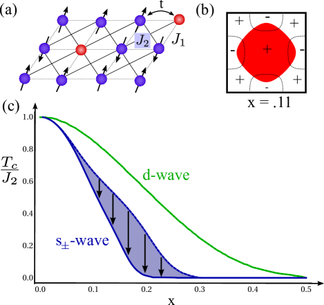
Figure 2: (a) The $t_{1}-J_{2}$ model. (b) The Fermi surface (holes shown in red) for the $t_{1}-J_{2}$ model at intermediate doping. In the superconducting state, the gap nodes follow the dashed lines, separating regions of positive and negative gap. (c) The superconducting transition temperatures for the $t_{1}-J_{2}$ model both with (solid lines) and without the $\lambda_{1}$ constraint(dashed lines), for s-wave (blue) and d-wave (green) superconductivity. d-wave superconductivity is unaffected by the Coulomb repulsion, while the s-wave transition temperature is decreased.

Now let us see this constraint in action, applied to several simple cases. First, we shall take the simplest lattice to exhibit $s_{\pm}$ pairing: the $t_{1}-J_{2}$ model shown in Fig. 2 (a). Here, only the next-nearest exchange coupling, $J_{2}$ and nearest neighbor hopping, $t_{1}$ are nonzero, which leads to a single hole Fermi surface with the potential for either $d_{xy}$ or $s_{\pm}$ pairing. The superconducting transition temperatures can be determined by setting $\Delta_{2s/d}=0^{+}$ and solving the mean field equations, (38) for $T_{c}$. The results are shown in Fig. 2(c), where we have calculated the transition temperatures as a function of doping, $x$ both with and without the $\lambda_{1}$ constraint. The d-wave transition temperature is unaffected, as $\partial F/\partial\lambda_{1}=0$ by symmetry, but the s-wave $T_{c}$ is suppressed. Note that the two transition temperatures are identical for $x=0$. Looking at the gap structure, Figure 2(b), we see that $\lambda_{1}$ has adjusted the gap nodes such that there are equal amounts of positive and negative gap density of states, eliminating the Coulomb repulsion. As there is only one Fermi surface in this example, there are necessarily line nodes even in the s-wave state. The energetic advantage of a fully gapped s-wave Fermi surface is thus lost, so that d-wave superconductivity, which requires no costly adjustment of the nodes, becomes energetically favorable for this lattice.

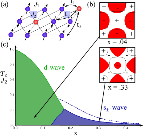
Figure 3: (a) The $t_{1}-t_{2}-t_{3}-J_{2}$ model. (b) The Fermi surface (holes shown in red) for the $t_{1}-t_{2}-t_{3}-J_{2}$ model at both low (single Fermi pocket) and intermediate doping (two Fermi pockets). The gap nodes of the superconducting state are indicated with dashed lines. (c) The doping phase diagram for the $t_{1}-t_{2}-t_{3}-J_{2}$ model, calculated with the $\lambda_{1}$ constraint (solid lines) and without (dashed lines). There is a quantum phase transition between d-wave pairing (green) and s-wave pairing (blue) as doping increases and the s-wave states become fully gapped.

However, if there are multiple Fermi surfaces, $s_{\pm}$ superconductivity can gap out both surfaces with opposite signs. If we tune the $t_{1}-t_{2}-t_{3}$ hoppings, keeping only $J_{2}$, we can obtain such a Fermi surface, with two hole pockets, as shown in Figure 3(a,b). Again, we calculate the s-wave and d-wave transition temperatures in the presence of the pseudopotential terms, showing the phase diagram in Figure 3(c). Our one-band approach makes this difficult, as the size of the pockets shrinks with increasing doping. The s-wave order parameter has line nodes for low doping, which recede to point nodes and then vanish as the Fermi surface becomes fully gapped at larger dopings, where the s-wave superconductivity is more favorable than d-wave, causing a d-wave to s-wave quantum phase transition as a function of doping. If we had equally balanced hole and electron pockets at zero doping, s-wave would likely win out over d-wave at all dopings.

V Discussion

This study of the symplectic-$N$ t-J model illustrates the importance of incorporating the Coulomb pseudopotential into any strongly correlated treatment of $s_{\pm}$ superconductors. The symplectic-$N$ scheme provides the first mean field solution of the $t-J$ model that is both controlled and superconducting. The large-$N$ limit is identical to previous mean-field studieskotliarliu88 , but contains the additional constraint fields $\lambda_{\pm}$ which enforce the constraint $\vec{\Psi}=0$. For d-wave pairing, this constraint is inert, as the s-wave component of the pairing is zero by symmetry, but this constraint plays a very active role for s-wave pairing, acting as a pair chemical potential that adjusts the gap nodes to eliminate any on-site pairing. As such, these models can capture the full variety of gap physics proposed in the iron-based superconductors: from line nodes to point nodes to two different full gaps that are not otherwise expected in a local picture. Properly accounting for the adjustment of the line nodes is essential when comparing the relative energies of d-wave and s-wave pairing states.

However, the large-$N$ limit suffers from an over-abundance of coherence, due to the ubiquity of the boson condensation. As such, the only phases captured here are Fermi liquids and superconductors, and studying the effects of $1/N$ corrections is an important future direction. This application is especially relevant to the cuprates, where there have been many intesting, but uncontrolled corrections to the mean field theories, revealing pseudogap-like phases formed by pre-formed pairs and incoherent metallic regionswenlee96 ; lee06 . A controlled $1/N$ study of the phase diagram of the $t-J$ model studying the differences between s-wave and d-wave pairing should be of great interest.

While the $t-J$ models taken in this paper illustrate the basic effect of the Coulomb pseudopotential on strongly correlated superconductors, they are but poor approximations of the real materials, due to the single band approximation. A better theory would involve multiple orbitals per site coupled by a ferromagnetic Hund’s coupling, $-|J_{H}|\vec{S}_{\mu i}\cdot\vec{S}_{\mu^{\prime}i}$ between spins in different orbitals, $\mu\neq\mu^{\prime}$ on the same site. Current large-$N$ techniques cannot treat such a ferromagnetic coupling, but future work might introduce an uncontrolled mean field parameter or take $J_{H}\rightarrow\infty$, which may prove more tractable.

Interestingly, while the majority of the iron-based superconductors have at least two electron and hole pockets, there are a handful of “single band” materials: there are the end members KFe₂As₂rotter08b and K_1-xFe_2-ySe₂guo10 , which appear to have only holesato09 or electron pocketsqian11 , respectively; and the single layer FeSe, which has a single electron pocketwang12 ; liu12 . In this local treatment, KFe₂As₂’s single hole pocket must lead to a nodal d-wave superconductorKFA , as in the $t-J_{2}$ example above, where the $s_{\pm}$ transition temperature is always smaller than the $d$-wave temperature. A d-wave gap is strongly suggested by recent heat conductivity measurementsreid12 . On the other hand, K_1-xFe_2-ySe₂ and single-layer FeSe have electron pockets, which can develop node-less $d$-wave order, as originally discussed from the weak coupling approachmazin11 ; wang11 ; maier11 . Including the Coulomb pseudopotential could again become important in this $d$-wave system if the tetragonal symmetry were broken.

Finally, an intriguing open problem in the iron-based superconductors is the relationship between the local quantum chemistry and the superconducting orderong11 . The strong dependence of the superconducting transition temperature on the Fe-As angledai08 ; yamada08 suggests that there might be a more local origin of superconductivity, similar to the composite pairs found in heavy fermion materials described by the two-channel Kondo latticeflint08 . These two origins of $s_{\pm}$ pairing could then work in tandem to raise the superconducting transition temperatureflint10 , and as such a future generalization of this work to take into account both the local iron chemistry and the staggered tetrahedral structure is highly desirable. Such tandem pairing might explain the robustness of these superconductors to disorder on the magnetic iron site hhwen .

Acknowledgments. The authors wish to acknowledge discussions with Andriy Nevidomskyy, Rafael Fernandes and Valentin Stanev related to this work. This work was supported by DOE grant DE-FG02-99ER45790.

VI Appendix

In this section, we show that the operator combination

$${\cal C} = \frac{1}{2}S_{\alpha\beta}S_{\beta\alpha}+[X_{0\alpha},X_{\alpha 0}]-(\tilde{X}_{00})^{2}$$ (42)

commutes with the Hubbard operators, where $\tilde{X}_{00}=X_{00}+1$. ${\cal C}$ is therefore the quadratic casimir of the symplectic supergroup SP(N$|$1). We also show that

$$C=(N/2)^{2}-1-\vec{\Psi}_{j}^{2}$$ (43)

in the symplectic slave boson representation.

The Hubbard operators $X_{0\alpha}$, $X_{\alpha 0}$ and $X_{00}$, together with the symplectic spin operators, $S_{\alpha\beta}=X_{\alpha\beta}-\frac{1}{N}X_{\lambda\lambda}$, form a closed superalgebra:

$$[S_{\alpha\beta},S_{\gamma\delta}] = \delta_{\beta\gamma}S_{\alpha\delta}-\delta_{\gamma\beta}S_{\alpha\delta}+\delta_{\bar{\beta}\delta}\tilde{\gamma}\tilde{\beta}S_{\alpha\bar{\gamma}}-\delta_{\gamma\bar{\alpha}}\tilde{\alpha}\tilde{\delta}S_{\bar{\delta}\beta}$$ (44)

$$[X_{0\alpha},S_{\beta\gamma}] = X_{0\gamma}\delta_{\alpha\beta}+\tilde{\alpha}\tilde{\beta}X_{0\bar{\beta}}\delta_{\alpha\bar{\gamma}}$$ (45)

$$\{X_{0\alpha},X_{\beta 0}\} = S_{\beta\alpha}+\delta_{\alpha\beta}\tilde{X}_{00}$$ (46)

$$\{X_{0\alpha},X_{0\beta}\} = 0$$ (47)

$$[X_{0\alpha},{X}_{00}] = -X_{0\alpha}.$$ (48)

Greek indices indicate spin indices $\alpha\in[\pm 1/2,\pm 3/2,\pm j]$ where $j=N/4$ and $N$ is even. For simplicity, we use the notation $\bar{\alpha}=-\alpha$ and $\tilde{\alpha}={\rm sgn}(\alpha)$. The operator $S_{\alpha\beta}=X_{\alpha\beta}-\frac{1}{N}\delta_{\alpha\beta}X_{\lambda\lambda}$ is the traceless symplectic spin operator, while the subsiduary operator, $\tilde{X}_{00}=X_{00}-\frac{1}{N}\sum_{\alpha}X_{\alpha\alpha}$. This graded Lie algebra defines the properties of the generators of the symplectic supergroup SP(N$|$1). This superalgebra is faithfully reproduced by the slave boson representation

$$X_{\alpha\beta} = f^{\dagger}_{\alpha}f_{\beta}+\tilde{\alpha}\tilde{\beta}f_{\bar{\alpha}}f^{\dagger}_{\bar{\beta}}$$ (49)

$$X_{\alpha 0} = f^{\dagger}_{\alpha}b+\tilde{\alpha}f_{\bar{\alpha}}a$$ (50)

$$X_{0\alpha} = b^{\dagger}f_{\alpha}+a^{\dagger}\tilde{\alpha}f_{\bar{\alpha}}$$ (51)

$$X_{00} = b^{\dagger}b+a^{\dagger}a$$ (52)

while the spin and subsiduary operator, $\tilde{X}_{00}$ are given by

$$S_{\alpha\beta} = X_{\alpha\beta}-\frac{1}{N}\delta_{\alpha\beta}X_{\lambda\lambda}=f^{\dagger}_{\alpha}f_{\beta}-\tilde{\alpha}\tilde{\beta}f^{\dagger}_{\bar{\beta}}f_{\bar{\alpha}}$$ (53)

$$\tilde{X}_{00} = X_{00}+\frac{1}{N}X_{\alpha\alpha}=b^{\dagger}b+a^{\dagger}a+1.$$ (54)

By inspection, ${\cal C}$ contains only rotationally invariant combinations of the Hubbard operators and each term leaves the number of slave bosons unchanged, so that it commutes with $S_{\alpha\beta}$ and $X_{00}$. We now show by direct evaluation that it also commutes with the fermionic Hubbard operators $X_{0\alpha}$ and $X_{\alpha 0}$

First we evaluate the commutator between $X_{\alpha 0}$ and the spin part of the Casimir,

$$[X_{0\alpha},S_{\beta\gamma}S_{\gamma\beta}] = [X_{0\alpha},S_{\beta\gamma}]S_{\gamma\beta}+S_{\beta\gamma}[X_{0\alpha},S_{\gamma\beta}]$$ (55)

$$= X_{0\gamma}S_{\gamma\alpha}+X_{0\bar{\beta}}S_{\bar{\alpha}\beta}{\rm sgn}(\alpha\beta)$$ (56)

$$+ S_{\beta\alpha}X_{0\beta}+{\rm sgn}(\alpha\gamma)S_{\bar{\alpha}\gamma}X_{0\bar{\gamma}}$$ (57)

Using the identity $S_{\alpha\beta}=-{\rm sgn}(\alpha\beta)S_{\bar{\beta}\bar{\alpha}}$, we can convert this expression into the form

$$[X_{0\alpha},S_{\beta\gamma}S_{\gamma\beta}] = X_{0\gamma}S_{\gamma\alpha}+X_{0\bar{\beta}}S_{\bar{\beta}\alpha}+S_{\beta\alpha}X_{0\beta}+S_{\bar{\gamma}\alpha}X_{0\bar{\gamma}}$$ (58)

$$= 2\{X_{0\beta},S_{\beta\alpha}\}.$$ (59)

Next we evaluate

$$-[X_{0\alpha},[X_{0\beta},X_{\beta 0}]] = -X_{0\beta}\{X_{0\alpha},X_{\beta 0}\}-\{X_{0\alpha},X_{\beta 0}\}X_{0\beta}$$ (60)

$$= -\{X_{0\beta},S_{\beta\alpha}\}-\{X_{0\alpha},\tilde{X}_{00}\}.$$ (61)

Finally,

$$[X_{0\alpha},\tilde{X}_{00}^{2}] = -[X_{0\alpha},\tilde{X}_{00}]\tilde{X}_{00}-\tilde{X}_{00}[X_{0\alpha},\tilde{X}_{00}]$$ (62)

$$= \{X_{0\alpha},\tilde{X}_{00}\}$$ (63)

Adding (58), (60) and (62) together gives

$$[X_{0\alpha},{\cal C}]=0.$$ (64)

Since $X_{\alpha 0}=X^{\dagger}_{0\alpha}$ and ${\cal C}={\cal C}^{\dagger}$ is Hermitian, it follows that $[X_{\alpha 0},{\cal C}]=0.$ Thus, ${\cal C}$ commutes with all Hubbard operators, and is thus a Casimir of the supergroup SP(N$|$1) generated by the symplectic operators.

To evaluate the Casimir, we insert the slave boson form of the Hubbard operators. First, evaluating the spin part, we obtain

$$S_{\alpha\beta}S_{\beta\alpha} = 2[f^{\dagger}_{\alpha}f_{\beta}f^{\dagger}_{\beta}f_{\alpha}-f^{\dagger}_{\bar{\beta}}f_{\bar{\alpha}}f^{\dagger}_{\beta}f_{\alpha}{\rm sgn}(\alpha\beta)]$$ (65)

$$= 2\left[f^{\dagger}_{\alpha}(N-f^{\dagger}_{\beta}f_{\beta})f_{\alpha}+f^{\dagger}_{\bar{\beta}}f^{\dagger}_{\beta}f_{\bar{\alpha}}f_{\alpha}{\rm sgn}(\alpha\beta)\right]$$ (66)

$$= 2\left[n_{f}(N+2-n_{f})-4\Psi^{\dagger}_{f}\Psi_{f}\right]$$ (67)

where $\Psi_{f}^{\dagger}=\sum_{\alpha>0}\tilde{\alpha}f^{\dagger}_{\bar{\alpha}}f^{\dagger}_{\alpha}$, while

$$\left[X_{0\alpha},X_{\alpha 0}\right] = (N-2n_{f})(n_{b}-n_{a})-N.$$ (68)

Combining the various terms in the Casimir, we obtain

$${\cal C} = n_{f}(N+2-n_{f})-(N-2n_{f})(n_{b}-n_{a})-N$$ (69)

$$- 4(\Psi^{\dagger}_{f}+b^{\dagger}a)(\Psi_{f}+a^{\dagger}b)+4b^{\dagger}aa^{\dagger}b-(\tilde{X}_{00})^{2}.$$ (70)

By regrouping terms, we obtain

$${\cal C} = -(n_{f}+n_{b}-n_{a}-\frac{N}{2})^{2}+(n_{b}-n_{a})^{2}+\left(\frac{N}{2}\right)^{2}$$ (71)

$$+ 2(n_{f}+n_{b}-n_{a}-\frac{N}{2})-2(n_{b}-n_{a})$$ (72)

$$- \Psi^{\dagger}\Psi+4b^{\dagger}aa^{\dagger}b-(\tilde{X}_{00})^{2}.$$ (73)

We now introduce the triad of operators

$$\Psi_{3} = n_{f}+n_{b}-n_{a}-\frac{N}{2}$$ (74)

$$\Psi^{\dagger} = \Psi^{\dagger}_{f}+b^{\dagger}a$$ (75)

$$\Psi = \Psi_{f}+a^{\dagger}b$$ (76)

where $[\Psi^{\dagger},\Psi]=\Psi_{3}$. Alternatively $\frac{1}{2}(\Psi_{1}+i\Psi_{2})=\Psi^{\dagger}$ and $\frac{1}{2}(\Psi_{1}-i\Psi_{2})=\Psi$. The Casimir can then be simplified to

$${\cal C} = -(\Psi_{3})^{2}+(n_{b}+n_{a}+1)^{2}+(N/2)^{2}-1$$ (77)

$$- (\Psi_{1}^{2}+\Psi_{2}^{2})-(n_{b}+n_{a}+1)^{2}$$ (78)

The terms involving $n_{b}$ and $n_{a}$ completely cancel out, leaving ${\cal C}=\left(\frac{N}{2}\right)^{2}-1-(\vec{\Psi}^{2}).$

References

- (1) Y. Kamihara, T. Watanabe, M. Hirano, and H. Hosono, J.Am. Chem. Soc. 130, 3296(2008).
- (2) J.W. Lynn, and P. Dai, Physica C 469, 469 (2009).
- (3) Q. Si and E. Abrahams, Phys. Rev. Lett. 101, 076401(2008).
- (4) K. Haule, J. H. Shim, G. Kotliar, Phys. Rev. Lett. 100, 226402 (2008).
- (5) A. Kutepov, K. Haule, S.Y. Savrasov, G. Kotliar,Phys. Rev. B 82, 045105 (2010).
- (6) I. I. Mazin, D. J. Singh, M. D. Johannes, and M. H. Du, Phys. Rev. Lett. 101, 057003 (2008).
- (7) A.V. Chubukov, D.V. Efremov, and I. Eremin, Phys. Rev. B 78, 134512(2008).
- (8) K. Seo, B. A. Bernevig, and J. Hu, Phys. Rev. Lett. 101, 206404 (2008).
- (9) M. M. Parish, J. Hu, and B. A. Bernevig, Phys. Rev. B 78, 144514 (2008).
- (10) T.A. Maier, S. Graser, D.J. Scalapino, P.J. Hirschfeld, Phys. Rev. B 79, 224510 (2009).
- (11) F. Wang, H. Zhai, Y. Ran, A. Vishwanath, and D.-H. Lee, Phys. Rev. Lett. 102, 1047005 (2009).
- (12) R. Sknepnek, G. Samolyuk, Y. Lee, J. Schmalian, Phys. Rev. B 79, 054511 (2009).
- (13) Z.-J. Yao, J.-X. Li, and Z. D. Wang, New J. Phys. 11, 025009 (2009).
- (14) Jiangping Hu, Hong Ding arXiv:1107.1334v1 (2011).
- (15) P. J. Hirschfeld, M. M. Korshunov and I. I. Mazin, Rep. Prog. Phys. 74, 124508 (2011).
- (16) P. Morel and P.W. Anderson, Phys. Rev. 125, 1263 (1962).
- (17) I.I. Mazin and J. Schmalian, Physica C., 469, 614(2009).
- (18) R. Flint, M. Dzero and P. Coleman, Nat. Phys. 4, 643 (2008).
- (19) R.Flint and P. Coleman, Phys. Rev. B 79, 014424(2009).
- (20) Rebecca Flint, Andriy Nevidomskyy and Piers Coleman, Phys. Rev. B 84, 064514 (2011).
- (21) J. Spalek, Physica B, 86-88, 375 (1977).
- (22) P.W. Anderson, Science 235, 118(1987).
- (23) G. Kotliar and J. Liu, Phys. Rev. B 38, 5142(1988).
- (24) X.G. Wen and P.A. Lee, Phys. Rev. Lett. 76, 503 (1996).
- (25) For an extensive review, see P. A. Lee, N. Nagaosa, and X.G. Wen, Rev. Mod. Phys. 78, 17 (2006).
- (26) P. Coleman, Phys. Rev. B 28, 5255 (1983).
- (27) I. Affleck and J.B. Marston, Phys. Rev. B 37, 3774(1988).
- (28) P. Coleman, C. Pépin and J. Hopkinson , Phys. Rev. B 63, 140411(R) (2001).
- (29) M. Rotter, M. Pangerl, M. Tegel, and D. Johrendt: Angew. Chem., Int.Ed. 47, 7949 (2008).
- (30) J.-G. Guo et al., Phys. Rev. B 82, 180520(R) (2010).
- (31) T. Sato et al, Phys. Rev. Lett. 103, 047002 (2009).
- (32) T. Qian et al, Phys. Rev. Lett. 106, 187001 (2011).
- (33) Q. Y. Wang et al, Chin. Phys. Lett. 29, 037402 (2012).
- (34) D. Liu et al, arXiv:1202.5849 (2012).
- (35) Nodal d-wave order is also predicted by weak-coupling approaches: R. Thomale et al., Phys. Rev. Lett. 107, 117001 (2011);S. Maiti et al., Phys. Rev. Lett. 107, 147002 (2011); K. Suzuki et al., Phys. Rev. B 84, 144514 (2011).
- (36) J.-Ph. Reid et al, arxiv:1201.3376 (2012).
- (37) I.I. Mazin, Phys. Rev. B84, 024529 (2011).
- (38) Fa Wang et al, Europhy. Lett. 93, 57003 (2011).
- (39) T.A. Maier, S. Graser, P.J. Hirschfeld, D.J. Scalapino, Phys. Rev. B 83, 100515(R) (2011).
- (40) T. Tzen Ong, Piers Coleman arxiv:1109.4131 (2011).
- (41) P. Dai, et. al. Nature Mat. 7, 953 (2008).
- (42) K. Yamada, et. al. J. Phys. Soc. Jpn 77, 083704 (2008).
- (43) R. Flint and P. Coleman, Phys. Rev. Lett. 105, 246404(2010).
- (44) H. Yang, Z. Wang, D. Fang, T. Kariyado, G. Chen, M. Ogata, T. Das, A. V. Balatsky, H. Wen, arXiv:1203.3123 (2012).
- (45) M. Vojta and S. Sachdev Phys. Rev. Lett. 83, 3916–3919 (1999); M. Vojta, Y. Zhang and S. Sachdev Phys. Rev. B 62, 6721–6744 (2000);