${\mathcal{PT}}$-symmetric deformations of integrable models

Abstract:

We review recent results on new physical models constructed as ${\mathcal{PT}}$-symmetrical deformations or extensions of different types of integrable models. We present non-Hermitian versions of quantum spin chains, multi-particle systems of Calogero-Moser-Sutherland type and non-linear integrable field equations of Korteweg-de-Vries type. The quantum spin chain discussed is related to the first example in the series of the non-unitary models of minimal conformal field theories. For the Calogero-Moser-Sutherland models we provide three alternative deformations: A complex extension for models related to all types of Coxeter/Weyl groups; models describing the evolution of poles in constrained real valued field equations of non-linear integrable systems and genuine deformations based on antilinearly invariant deformed root systems. Deformations of complex nonlinear integrable field equations of KdV-type are studied with regard to different kinds of ${\mathcal{PT}}$-symmetrical scenarios. A reduction to simple complex quantum mechanical models currently under discussion is presented.

1 Introduction

Until fairly recently [1] non-Hermitian systems have been mostly viewed as not self-consistent descriptions of dissipative systems. However, in constrast to the previous misconception it is by now well understood that Hamiltonians admitting an antilinear symmetry may be used to define consistent classical, quantum mechanical and quantum field theoretical systems. Various techniques have been developed to achieve this. Central to this is construction of metric operators such that certain quantities in the models can be viewed as physical observables [2, 3, 4, 5, 6, 7, 8, 9, 10, 11]. In particular, it was found that such type of models models possess real energy spectra in large sectors in their parameter space, despite being non-Hermitian. The explanation for this property can be traced back to an observation made by Wigner more than fifty years ago [12], who notices that operators invariant under antilinear transformations possess either real eigenvalues or eigenvalues occurring in complex conjugate pairs depending on whether their eigenfunctions also respect this symmetry or not, respectively. A very explicit example of such a symmetry is a simultaneous parity transformation $\mathcal{P}$ and time reversal $\mathcal{T}$. This $\mathcal{PT}$-symmetry is trivially verified for instance for Hamiltonian operators $H$, but less obvious for the corresponding wavefunctions $\psi$ due to the fact that often they are not known explicitly. When

$$\left[H,\mathcal{PT}\right]=0\qquad\text{and\qquad}\mathcal{PT}\psi=\psi$$ (1)

hold one speaks of a $\mathcal{PT}$-symmetric system, but when only the first relation holds one speaks of spontaneously broken $\mathcal{PT}$ -symmetry and when none of the relations in (1) holds of broken $\mathcal{PT}$-symmetry. Here we will view the $\mathcal{PT}$-operator in a wider sense and refer to it loosely as $\mathcal{PT}$ even when it is not strictly a reflection in time and space, but when it is an antilinear involution satisfying

$$\mathcal{PT}\left(\alpha\psi+\beta\phi\right)=\alpha^{\ast}\mathcal{PT}\psi+\beta^{\ast}\mathcal{PT}\phi\qquad\text{for }\alpha,\beta\in\mathbb{C}\text{, \ \ \ \ \ }\mathcal{PT}^{2}=\mathbb{I}.$$ (2)

Very often synonymously used, even though conceptually quite different, are the notions of quasi-Hermiticity [13, 14, 2] and pseudo-Hermiticity [15, 16, 4]. These concepts refer more directly to the properties of the metric operator and their subtle difference is often overlooked, even though this is very important as they allow for different types of conclusions. In the quasi-Hermitian case the metric operator is positive and Hermitian, but not necessarily invertible. It was shown [13, 14, 2] that in this case the existence of a definite metric is guaranteed and the eigenvalues of the Hamiltonian are real. The pseudo-Hermitian scenario, that is dealing with an invertible Hermitian, but not necessarily positive metric, is less appealing as the eigenvalues are only guaranteed to be real but no definite conclusions can be reached with regard to the existence of a definite metric. Thus in this latter case the status and consistency of the corresponding quantum theory remain inconclusive.

Even though some fundamental questions remain partially unanswered, such as the puzzle concerning the uniqueness of the metric or the question of what constitutes a good set of ingredients to formulate a consistent physical theory, the understanding is general in a very mature state. So far it could be used to revisit some old theories, which had either been discarded as being non-physical or had considerable gaps in their treatment, and put them on more solid ground. Another interesting possibility which had opened up through these studies is the formulation of entirely new models based on non-Hermitian Hamiltonians which however possess the desired $\mathcal{PT}$-symmetry. In other words, one may use the $\mathcal{PT}$-symmetry to deform or extend previously studied models and thus obtain large sets of entirely unexplored theories. In principle, this kind of programme can be carried out in any area of physics. Here we will explore how these ideas can be used in the context of integrable models. We will not report here on how well established methods from integrable systems can be applied to study non-Hermitian quantum mechanical models [17], even though we will report some scenarios in which they naturally emerge as reduced integrable systems [18]. Instead we present here how these ideas have been used so far to formulate and study new models previously overlooked as they would have been regarded as non-physical due to their non-Hermitian nature. We present results on standard types of integrable models, a quantum spin-chain, multi-particle systems of Calogero type and nonlinear wave equations of KdV-type.

The construction principle is fairly simple. Identifying some anti-symmetric operators $\mathcal{O}$ in the system, we seek a deformation map $\delta_{\varepsilon}$ of the form

$$\mathcal{PT}:\mathcal{O}\mapsto-\mathcal{O}\quad\Rightarrow\quad\delta_{\varepsilon}:\mathcal{O}\mapsto-i(i\mathcal{O)}^{\varepsilon},$$ (3)

with $\varepsilon$ being a deformation parameter such that the non-deformed model is recovered in the limit $\varepsilon\rightarrow 1$. Alternatively one can also just add $\mathcal{PT}$-symmetric terms to the original system and regard them as perturbations.

2 $\mathcal{PT}$-symmetrically deformed quantum spin chains

Quantum spin chains constitute a good starting point since, being just finite matrix models, they can be viewed in many ways as the easiest integrable models. We present here a model which has been considered first by von Gehlen [19], that is an Ising quantum spin chain in the presence of a magnetic field in the $z$-direction as well as a longitudinal imaginary field in the $x$-direction. The corresponding Hamiltonian for a chain of length $N$ acting on a Hilbert space of the form $(\mathbb{C}^{2})^{\otimes N}$ is given by

$$H(\lambda,\kappa)=-\frac{1}{2}\sum_{j=1}^{N}(\sigma_{j}^{z}+\lambda\sigma_{j}^{x}\sigma_{j+1}^{x}+i\kappa\sigma_{j}^{x}),\qquad\lambda,\kappa\in\mathbb{R}.$$ (4)

We used the standard notation for the $2^{N}\times 2^{N}$-matrices $\sigma_{i}^{x,y,z}=\mathbb{I\otimes I\otimes\ldots\otimes}\sigma^{x,y,z}\otimes\ldots\otimes\mathbb{I\otimes I}$ with Pauli matrices

$$\sigma^{x}=\left(\begin{array}[]{cc}0&1\\ 1&0\end{array}\right),\qquad\sigma^{y}=\left(\begin{array}[]{cc}0&-i\\ i&0\end{array}\right),\qquad\sigma^{z}=\left(\begin{array}[]{cc}1&0\\ 0&-1\end{array}\right),$$ (5)

describing spin 1/2 particles as $i$-th factor acting on the site $i$ of the chain. This model is of interest as it can be viewed [20] as a perturbation of the $\mathcal{M}_{5,2}$-model in the $\mathcal{M}_{p,q}$-series of minimal conformal field theories [21]. It is the simplest non-unitary model in this infinite class of models, which are all characterized by the condition $p-q>1$ and whose corresponding Hamiltonians are all expected to be non-Hermitian. The $\mathcal{PT}$-symmetry of the model was exploited in [22].

2.1 Different versions of $\mathcal{PT}$-symmetry

Let us first identify the $\mathcal{PT}$-symmetry for the Hamiltonian (4). Non-Hermitian spin chains have first been studied in this regard in [23], where the parity operator $\mathcal{P}^{\prime}:\sigma_{i}^{x,y,z}\rightarrow\sigma_{N+1-i}^{x,y,z}$ was interpreted quite literally as a reflection about the center of the chain. Viewing ${\mathcal{T}}$ as a standard complex conjugation $\mathcal{P}^{\prime}{\mathcal{T}}$ is then easily identified as a symmetry of the $XXZ$-spin chain Hamiltonian $H_{XXZ}$. However, it is seen immediately that this operator is not a symmetry of the Hamiltonian $H(\lambda,\kappa)$ in (4). Defining instead [22] the operator

$$\mathcal{P}:=\prod\limits_{i=1}^{N}\sigma_{i}^{z},\quad\text{with }\quad\mathcal{P}^{2}=\mathbb{I}^{\otimes N},$$ (6)

as an analogue to the parity operator, we may carry out a site-by-site reflection

$$\mathcal{P}:(\sigma_{i}^{x},\sigma_{i}^{y},\sigma_{i}^{z})\rightarrow(-\sigma_{i}^{x},-\sigma_{i}^{y},\sigma_{i}^{z})\quad\text{and\quad}\mathcal{T}:(\sigma_{i}^{x},\sigma_{i}^{y},\sigma_{i}^{z})\rightarrow(\sigma_{i}^{x},-\sigma_{i}^{y},\sigma_{i}^{z}).$$ (7)

It is then easy to verify that this operator is a symmetry of $H(\lambda,\kappa)$, i.e. we have $\left[\mathcal{PT},H(\lambda,\kappa)\right]=0$. Clearly this $\mathcal{PT}$-operator acts antilinearly satisfying (2) and is therefore a viable candidate for our purposes. In analogy to (6) it is then also suggestive to define

$$\mathcal{P}_{x}:=\prod\limits_{i=1}^{N}\sigma_{i}^{x}\qquad\text{and\qquad}\mathcal{P}_{y}:=\prod\limits_{i=1}^{N}\sigma_{i}^{y},$$ (8)

which act as

$$\mathcal{P}_{x/y}:(\sigma_{i}^{x},\sigma_{i}^{y},\sigma_{i}^{z})\rightarrow(\pm\sigma_{i}^{x},\mp\sigma_{i}^{y},-\sigma_{i}^{z}).$$ (9)

One can verify that $\left[\mathcal{P}_{x/y}\mathcal{T},H(\lambda,\kappa)\right]\neq 0$ and $\left[\mathcal{P}_{x/y}\mathcal{T},H_{XXZ}\right]=0$. Similar properties can be observed for the non-Hermitian quantum spin chain [24]

$$H_{DG}=\sum_{i=1}^{N}\left(\kappa_{zz}\sigma_{i}^{z}\sigma_{i+1}^{z}+\kappa_{x}\sigma_{i}^{x}+\kappa_{y}\sigma_{i}^{y}\right),$$ (10)

with $\kappa_{zz}\in\mathbb{R}$ and $\kappa_{x}$, $\kappa_{y}\in\mathbb{C}$. Clearly when $\kappa_{x}$ or $\kappa_{y}\notin\mathbb{R}$ the Hamiltonian $H_{DG}$ is not Hermitian, but once again one can find suitable symmetry operators. We notice that $\left[\mathcal{P}^{\prime}\mathcal{T},H\right]\neq 0$, whereas $\left[\mathcal{PT},H\right]=0$ for $\kappa_{x},\kappa_{y}\in i\mathbb{R}$ and $\left[\mathcal{P}_{x/y}\mathcal{T},H\right]=0$ for $\kappa_{x/y}\in\mathbb{R},\kappa_{y/x}\in i\mathbb{R}$.

Below we will encounter further ambiguities in the definition of the antilinear symmetry, which will all manifest in the non-uniqueness of the metric operator and therefore in the definition of the physics described by these models. For the Hamiltonians $H_{XXZ}$ and $H_{DG}$ the consequences of this fact are yet to be explored.

2.2 The two site model

It is instructive to commence with the simplest example for which all quantities of interest can be computed explicitly in a very transparent way. We specify at first the length of the chain to be $N=2$ and without loss of generality fix the boundary conditions to be periodic $\sigma_{N+1}^{x}=\sigma_{1}^{x}$. The Hamiltonian (4) then acquires the simple form of a non-Hermitian $(4\times 4)$-matrix

$$H_{2}(\lambda,\kappa) = -\frac{1}{2}\left[\sigma_{z}\otimes\mathbb{I}+\mathbb{I}\otimes\sigma_{z}+2\lambda\sigma_{x}\otimes\sigma_{x}+i\kappa\left(\mathbb{I}\otimes\sigma_{x}+\sigma_{x}\otimes\mathbb{I}\right)\right],$$ (11)

$$= -\left(\begin{array}[]{rrrr}-1&\frac{i\kappa}{2}&\frac{i\kappa}{2}&\lambda\\ \frac{i\kappa}{2}&0&\lambda&\frac{i\kappa}{2}\\ \frac{i\kappa}{2}&\lambda&0&\frac{i\kappa}{2}\\ \lambda&\frac{i\kappa}{2}&\frac{i\kappa}{2}&-1\end{array}\right).$$ (16)

The characteristic polynomial for (16) factorizes into a first and a third order polynomial such that the eigenvalues acquire a simple analytic form. Defining the domain

$$U_{\mathcal{PT}}=\left\{\lambda,\kappa:\kappa^{6}+8\lambda^{2}\kappa^{4}-3\kappa^{4}+16\lambda^{4}\kappa^{2}+20\lambda^{2}\kappa^{2}+3\kappa^{2}-\lambda^{2}-1\leq 0\right\}$$ (17)

in the parameter space, the $\mathcal{PT}$-symmetry is unbroken in the sense described by (1) when $(\lambda,$ $\kappa)\in U_{\mathcal{PT}}$. The four real eigenvalues are evaluated in this case to

$$\begin{array}[]{ccc}\varepsilon_{1}=\lambda,&\varepsilon_{2}=2q^{\frac{1}{2}}\cos\left(\frac{\theta}{3}\right)-\frac{\lambda}{3},&\varepsilon_{3/4}=2q^{\frac{1}{2}}\cos\left(\frac{\theta}{3}+\pi\mp\frac{\pi}{3}\right)-\frac{\lambda}{3},\end{array}$$ (18)

where

$$\theta=\arccos\left(\frac{r}{q^{3/2}}\right),\quad q=\frac{1}{9}\left(3+4\lambda^{2}-3\kappa^{2}\right),\quad r=\frac{\lambda}{27}\left(18\kappa^{2}+8\lambda^{2}+9\right).$$ (19)

We depict the eigenvalues in figure 1 for some fixed $\lambda$ or $\kappa$ and varying $\kappa$ or $\lambda$, respectively.

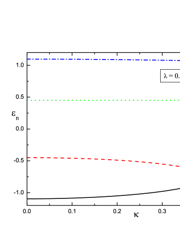
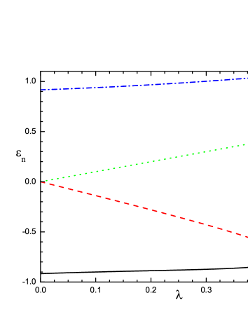
Figure 1: Unavoided level crossing: eigenvalues as functions of $\lambda$ ($\kappa$) for fixed $\kappa$ ($\lambda$) for $H_{2}(\lambda,\kappa)$.

We observe the typical behaviour for $\mathcal{PT}$-symmetric systems, namely that two eigenvalues start to coincide at the exceptional point [25] when $\kappa$ and $\lambda$ are situated on the boundary of $U_{\mathcal{PT}}$. Going beyond those values, the $\mathcal{PT}$-symmetry is spontaneously broken and the two merged eigenvalues develop into a complex conjugate pair. This is of course a phenomenon prohibited for standard Hermitian systems by the Wigner–von Neumann non-crossing rule [26].

For the Hamiltonian (11) one can compute explicitly the left $\left|\Phi_{n}\right\rangle$ and right eigenvectors $\left|\Psi_{n}\right\rangle$, forming a biorthonormal basis

$$\left\langle\Psi_{n}\right.\left|\Phi_{m}\right\rangle=\delta_{nm},\qquad\text{and\qquad}\sum\nolimits_{n}\left|\Phi_{n}\right\rangle\left\langle\Psi_{n}\right|=\mathbb{I}$$ (20)

and verify that indeed for the spontaneously broken regime the second relation in (1) does not hold, see [22] for the concrete expresssions. We have then all the ingredients to compute the metric operator $\rho$ and define the inner product $\langle.|.\rangle_{\rho}:=\langle.|\rho.\rangle$ with regard to which the Hamiltonian (11) is Hermitian

$$\langle\psi|H\phi\rangle_{\rho}=\langle H\psi|\phi\rangle_{\rho}.$$ (21)

Computing the signature $s=(s_{1},s_{2},\ldots,s_{n})$ from

$$\mathcal{P}\left|\Phi_{n}\right\rangle=s_{n}\left|\Psi_{n}\right\rangle\text{\qquad with }s_{n}=\pm 1$$ (22)

we may evaluate the so-called $\mathcal{C}$-operator introduced in [3]

$$\mathcal{C}:=\sum\nolimits_{n}s_{n}\left|\Phi_{n}\right\rangle\left\langle\Psi_{n}\right|,$$ (23)

and hence the metric operator $\rho$, which also relates the Hamiltonian to its conjugate

$$\rho:=\mathcal{PC},\mathcal{\qquad}H^{\dagger}\rho=\rho H.$$ (24)

The explicit expressions can be found in [22], from which one can verify explicitly that the metric operator is Hermitian, positive and invertible. Thus the Hamiltonian (11) is quasi-Hermitian as well as pseudo-Hermitian. From the expression for $\rho$ we can also obtain the so-called Dyson map $\eta$ [27], by taking the positive square root $\eta=\sqrt{\rho}$. This operator serves to construct an isospectral Hermitian counterpart $h$ to $H$ by its adjoint action. For (11) we find

$$h_{2}(\lambda,\kappa)=\eta H_{2}(\lambda,\kappa)\eta^{-1}=\sum\limits_{s=x,y,z}\nu_{s}\sigma_{s}\otimes\sigma_{s}+\mu_{z}(\sigma_{z}\otimes\mathbb{I}+\mathbb{I}\otimes\sigma_{z}).$$ (25)

The constants $\nu_{x}$, $\nu_{y}$, $\nu_{z}$ and $\mu_{z}$ can be found in [22].

2.3 Perturbative computation for the N-site model

It is clear that when proceeding to longer spin chains it becomes increasingly complex to compute the above mentioned operators such that exact computation become less transparent and can only be carried out with great effort. However, we may also gain considerable insight by resorting to a perturbative analysis. For this purpose we separate the Hamiltonian into its Hermitian and non-Hermitian part as $H(\lambda,\kappa)=h_{0}(\lambda)+i\kappa h_{1}$, where $h_{0}$ and $h_{1}$ are both Hermitian, with $\kappa$ being a real coupling constant as for instance introduced in (4). Assuming next that the inverse of the metric exists and that it can be parameterized as $\rho=e^{q}$, the second equation in (24) can be written as

$$H^{\dagger}=e^{q}He^{-q}=H+[q,H]+\frac{1}{2}[q,[q,H]]+\frac{1}{3!}[q,[q,[q,H]]]+\cdots$$ (26)

Presuming further that the metric can be perturbatively expanded as

$$q=\sum_{k=1}^{\infty}\kappa^{2k-1}q_{2k-1},$$ (27)

we obtain the following equations order by order in $\kappa$

$$[h_{0},q_{1}] = 2ih_{1},$$ (28)

$$[h_{0},q_{3}] = \frac{i}{6}[q_{1},[q_{1},h_{1}]],$$ (29)

$$[h_{0},q_{5}] = \frac{i}{6}[q_{1},[q_{3},h_{1}]]+\frac{i}{6}[q_{3},[q_{1},h_{1}]]-\frac{i}{360}[q_{1},[q_{1},[q_{1},[q_{1},h_{1}]]]].~{}~{}$$ (30)

It is clear from (28)-(30) that at each order one new unknown quantity enters the computation for which we can solve our equations, i.e. in (28) we solve for $q_{1}$ for known $h_{0}$ and $h_{1}$, in (29) for $q_{3}$, in (30) for $q_{5}$, etc. This process can be continued up to any desired order of precision, see [8] for further general details on perturbation theory.

Proceeding in this manner we compute the Dyson operator as described above and determine the Hermitian counterpart. For $N=3$ we obtain

$$h=\mu_{xx}^{3}S_{xx}^{3}+\mu_{yy}^{3}S_{yy}^{3}+\mu_{zz}^{3}S_{zz}^{3}+\mu_{z}^{3}S_{z}^{3}+\mu_{xxz}^{3}S_{xxz}^{3}+\mu_{yyz}^{3}S_{yyz}^{3}+\mu_{zzz}^{3}S_{zzz}^{3},$$ (31)

where for convenience we introduced a new notation

$$S_{a_{1}a_{2}\ldots a_{p}}^{N}:=\sum_{k=1}^{N}\sigma_{k}^{a_{1}}\sigma_{k+1}^{a_{2}}\ldots\sigma_{k+p-1}^{a_{p}},~{}~{}\text{for}~{}~{}a_{i}=x,y,z,u;~{}i=1,\ldots,p\leq N.$$ (32)

The coefficients $\mu_{xx},\ldots,\mu_{zzz}$ are real functions of the couplings $\lambda$ and $\kappa$. We denote here $\sigma^{u}=\mathbb{I}$ to allow for the possibility of non-local, i.e. not nearest neighbour, interactions. In fact, they do occur when we increase the length of the chain by one site. For $N=4$ we compute

$$h = \mu_{xx}^{4}S_{xx}^{4}+\nu_{xx}^{4}\mathbf{S}_{xux}^{4}+\mu_{yy}^{4}S_{yy}^{4}+\nu_{yy}^{4}\mathbf{S}_{yuy}^{4}+\mu_{zz}^{4}S_{zz}^{4}+\nu_{zz}^{4}\mathbf{S}_{zuz}^{4}+\mu_{z}^{4}S_{z}^{4}~{}~{}~{}~{}~{}$$ (33)

$$+\mu_{xxz}^{4}(S_{xxz}^{4}+S_{zxx}^{4})+\mu_{xzx}^{4}S_{xzx}^{4}+\mu_{yyz}^{4}(S_{yyz}^{4}+S_{zyy}^{4})+\mu_{yzy}^{4}S_{yzy}^{4}$$

$$+\mu_{zzz}^{4}S_{zzz}^{4}+\mu_{xxxx}^{4}S_{xxxx}^{4}+\mu_{yyyy}^{4}S_{yyyy}^{4}+\mu_{zzzz}^{4}S_{zzzz}^{4}+\mu_{xxyy}^{4}S_{xxyy}^{4}$$

$$+\mu_{xyxy}^{4}S_{xyxy}^{4}+\mu_{zzyy}^{4}S_{zzyy}^{4}+\mu_{zyzy}^{4}S_{zyzy}^{4}+\mu_{xxzz}^{4}S_{xxzz}^{4}+\mu_{xzxz}^{4}S_{xzxz}^{4}.\;\;$$

We observe that the first non-local interaction terms proportional to $S_{xux}^{4}$, $S_{yuy}^{4}$ and $S_{zuz}^{4}$ emerge in this model. Thus we encounter a very typical feature of non-Hermitian $\mathcal{PT}$-symmetric Hamiltonian systems, whereas the non-Hermitian Hamiltonian is fairly simple its Hermitian isospectral counterpart is quite complicated involving non-nearest neighbour interactions. An additional feature not present for chains of smaller length is the fact that some of the $\lambda$-dependence of the coefficients $\mu_{xx},\ldots,\mu_{xzxz}$ is no longer polynomial and gives rise to singularities.

This models exhibits the basic feature, but clearly there is plenty of scope left for further analysis. More explicit analytic formulae should be computed for $\eta$, $\rho$ and $h$ for longer chains, models with higher spin values should be considered and further members of the class belonging to the perturbed $\mathcal{M}_{p,q}$-series of minimal conformal field theories should be studied. Interesting recent results on other non-Hermitian quantum spin chains may be found in [28, 29].

3 $\mathcal{PT}$-symmetrically deformed Calogero type models

$\mathcal{PT}$-deformed versions of multi-particle systems of Calogero type have been obtained so far in three quite different ways, as simple extensions, as constrained field equations or as genuine deformations.

3.1 Extended Calogero-Moser-Sutherland models

The most direct and simplest way to obtain $\mathcal{PT}$-symmetrically extended versions of Calogero-Moser Sutherland models is to add a $\mathcal{PT}$-symmetric term to the original model as proposed in [30]

$$\mathcal{H}_{\mathcal{PT}CMS}=\frac{1}{2}p^{2}+\frac{1}{2}\sum\limits_{\alpha\in\Delta}g_{\alpha}^{2}V(\alpha\cdot q)+\frac{i}{2}\tilde{g}_{\alpha}f(\alpha\cdot q)\alpha\cdot p,$$ (34)

with coupling constants $g,\tilde{g}\in\mathbb{R}$, canonical variables $q,p\in\mathbb{R}^{\ell+1}$ for an $(\ell+1)$-dimensional representation of the roots $\alpha$ of some arbitrary root system $\Delta$, which is left invariant under the Coxeter group. The potential may take on different forms $V(x)=f^{2}(x)$ defined by means of the function $f(x)=1/x$, $f(x)=1/\sinh x$ or $f(x)=1/\sin x$. The model in (34) is a generalization of an extension of the $A_{\ell}$ and $B_{\ell}$-Calogero model, i.e. $f(x)=1/x$, for a specific representation of the roots as suggested in [31, 32, 33]. The $\mathcal{PT}$-symmetry of $\mathcal{H}_{\mathcal{PT}CMS}$ is easily verified. In [30] it was shown that for $f(x)=1/x$ one may re-write the Hamiltonian in (34), such that it becomes the standard Hermitian Calogero Hamiltonian with shifted momenta $p\rightarrow p+i\mu$

$$\mathcal{H}_{\mathcal{PT}CMS}=\frac{1}{2}(p+i\mu)^{2}+\frac{1}{2}\sum\limits_{\alpha\in\Delta}\hat{g}_{\alpha}^{2}V(\alpha\cdot q),$$ (35)

where $\mu:=1/2\sum\nolimits_{\alpha\in\Delta}\tilde{g}_{\alpha}f(\alpha\cdot q)\alpha$ and the coupling constants have been redefined to $\hat{g}_{\alpha}^{2}:=g_{s}^{2}+\alpha_{s}^{2}\tilde{g}_{s}^{2}$ for $\alpha\in\Delta_{s}$ and $\hat{g}_{\alpha}^{2}:=g_{l}^{2}+\alpha_{l}^{2}\tilde{g}_{l}^{2}$ for $\alpha\in\Delta_{l}$, where $\Delta_{l}$ and $\Delta_{s}$ refer to the root system of the long and short roots, respectively. This manipulation is based on the not obvious identity $\mu^{2}=\alpha_{s}^{2}\tilde{g}_{s}^{2}\sum\nolimits_{\alpha\in\Delta_{s}}V(\alpha\cdot q)+\alpha_{l}^{2}\tilde{g}_{l}^{2}\sum\nolimits_{\alpha\in\Delta_{l}}V(\alpha\cdot q)$, which is only valid for rational potentials. Even then it has not been proven yet in a case independent manner, but verified for many examples on a case-by-case basis [30].

For the rational potential it is straightforward to obtain the Dyson map $\eta=e^{-q\cdot\mu}$, which relates the standard Hermitian Calogero model to the non-Hermitian model (34) by an adjoint action $\mathcal{H}_{\mathcal{PT}C}=\eta^{-1}\mathcal{H}_{C}\eta$. The integrability of the rational version of $\mathcal{H}_{\mathcal{PT}CMS}$ follows then from the existence of the Lax pair $L_{C}$ and $M_{C}$ obeying the Lax equation $\dot{L}_{\mathcal{PT}C}=\left[L_{\mathcal{PT}C},M_{\mathcal{PT}C}\right]$, which maybe obtained from the standard Calogero Lax pair [34] as $L_{\mathcal{PT}C}(p)=\eta^{-1}L_{C}(p)\eta=$ $L_{C}(p+i\mu)$ and $M_{\mathcal{PT}C}(p)=\eta^{-1}M_{C}(p)\eta=$ $M_{C}(p+i\mu)$. Expanding the shifted kinetic term in (35) we obtain

$$\mathcal{H}_{\mathcal{PT}CMS}=\frac{1}{2}p^{2}+\frac{1}{2}\sum\limits_{\alpha\in\Delta}\hat{g}_{\alpha}^{2}V(\alpha\cdot q)+i\mu\cdot p-\frac{1}{2}\mu^{2}.$$ (36)

By the reasoning provided, it follows that this model is integrable for all of the above stated potential, whereas the model without the $\mu^{2}$-term is only integrable for rational potentials.

3.2 From constraint field equations to $\mathcal{PT}$-deformed Calogero models

Another more surprising way to obtain particle systems of complex Calogero type arises from considering real valued field solutions for some nonlinear equations. Making an Ansatz in form of a real valued field

$$u(x,t)=\frac{\lambda}{2}\sum\limits_{k=1}^{\ell}\left(\frac{i}{x-z_{k}(t)}-\frac{i}{x-z_{k}^{\ast}(t)}\right),\qquad\lambda\in\mathbb{R},$$ (37)

it was shown more than thirty years ago [35, 36] that this constitutes an $\ell$-soliton solution for the Benjamin-Ono equation

$$u_{t}+uu_{x}+\lambda Hu_{xx}=0,$$ (38)

with $Hu(x)$ denoting the Hilbert transform $Hu(x)=\frac{P}{\pi}\int_{-\infty}^{\infty}\frac{u(x)}{z-x}dz$, provided the poles $z_{k}$ in (37) obey the complex $A_{\ell}$-Calogero equation of motion

$$\ddot{z}_{k}=\frac{\lambda^{2}}{2}\sum\limits_{j\neq k}(z_{j}-z_{k})^{-3},\qquad z_{k}\in\mathbb{C}.$$ (39)

Clearly for different types of nonlinear equations the constraining equation might be of a more complicated form. However, we may consistently impose additional constraints by making use of the following theorem of Airault, McKean and Moser [37]:

Given a Hamiltonian $H(x_{1},\ldots,x_{n},\dot{x}_{1},\ldots,\dot{x}_{n})$ with flow

$$x_{i}={\partial H}/{\partial\dot{x}_{i}}\qquad\text{and\qquad}\ddot{x}_{i}=-{\partial H}/{\partial x_{i}}\qquad i=1,\ldots,n$$ (40)

and conserved charges $I_{j}$ in involution with $H$, i.e. vanishing Poisson brackets $\{I_{j},H\}=0$. Then the locus of grad $I=0$ is invariant with regard to time evolution. Thus it is permitted to restrict the flow to that locus provided it is not empty.

Making now the Ansatz

$$v(x,t)=\lambda\sum\limits_{k=1}^{\ell}{(x-z_{k}(t))^{-2}},\qquad\lambda\in\mathbb{R}$$ (41)

one can show that this solves the Boussinesq equation

$$v_{tt}=a(v^{2})_{xx}+bv_{xxxx}+v_{xx}\qquad a,b\in\mathbb{R}.$$ (42)

if and only if $b=1/12$, $\lambda=-a/2$ and the poles $z_{k}$ obeys the constraining equations

$$\ddot{z}_{k} = 2\sum\limits_{j\neq k}(z_{j}-z_{k})^{-3}\qquad\quad\Leftrightarrow\quad\ddot{z}_{k}=-\frac{\partial H_{Cal}}{\partial z_{i}},$$ (43)

$$\dot{z}_{k}^{2} = 1-\sum\limits_{j\neq k}(z_{j}-z_{k})^{-2}\qquad\Leftrightarrow\quad\mathtt{grad}(I_{3}-I_{1})=0.$$ (44)

Here $I_{3}=\sum_{j=1}^{\ell}[\dot{z}_{j}^{3}/3+\sum\nolimits_{k\neq j}\dot{z}_{j}(z_{j}-z_{k})^{2}]$ and $I_{1}=\sum_{j=1}^{\ell}\dot{z}_{j}$ are two conserved charges in the $A_{\ell}$-Calogero model. Thus in comparison with the previous example (37)-(38) we have to satisfy an additional constraints (44) besides the equations of motion of the $A_{\ell}$-Calogero model. However, according to the above theorem this is still a consistent system of equations, provided the equations (43) and (44) possess any non-trivial solution. Only very few solutions have been found so far. The simplest two-particle solution was already reported in [37]

$$z_{1}=\kappa+\sqrt{(t+\tilde{\kappa})^{2}+1/4},\qquad z_{2}=\kappa-\sqrt{(t+\tilde{\kappa})^{2}+1/4}.$$ (45)

In this case the Boussinesq solution acquires the form

$$v(x,t)=2\lambda\frac{(x-\kappa)^{2}+(t+\tilde{\kappa})^{2}+1/4}{[(x-\kappa)^{2}-(t+\tilde{\kappa})^{2}-1/4]^{2}}.$$ (46)

Note that $v(x,t)$ is still a real solution. However, without any complication we may change $\kappa$ and $\tilde{\kappa}$ to be purely imaginary in which case, and only in this case, (46) becomes a solution for the $\mathcal{PT}$-symmetric equation (42) in the sense that $\mathcal{PT}:x\rightarrow-x,t\rightarrow-t$ and $v\rightarrow v$. A three particle solution was reported in [38], which exhibits an interesting solitonic behaviour in the complex plane. In that case no real solution could be found and once again one was forced to consider complex particle systems. For more particles, different types of algebras or other types of nonlinear equations these investigations have not been carried out yet.

3.3 Deformed Calogero-Moser-Sutherland models

Let us now consider the $CMS$-models with an additional confining potential

$$\mathcal{H}_{\mathcal{PT}CMS}^{\prime}=\frac{p^{2}}{2}+\frac{m^{2}}{16}\sum_{\alpha\in\Delta_{s}}(\alpha\cdot\tilde{q})^{2}+\frac{1}{2}\sum\limits_{\alpha\in\Delta}g_{\alpha}V(\alpha\cdot\tilde{q}),\,\,~{}~{}~{}m,g_{\alpha}\in\mathbb{R},$$ (47)

and also deforme the coordinates $q\rightarrow\tilde{q}$. Considering at first the $A_{2}$-case for a standard three dimensional representation for the simple $A_{2}$-roots $\alpha_{1}=\{1,-1,0\}$, $\alpha_{2}=\{0,1,-1\}$, we deformed the coordinates as

$$q_{1} \rightarrow \tilde{q}_{1}=q_{1}\cosh\varepsilon~{}+i\sqrt{3}(q_{2}-q_{3})\sinh\varepsilon$$ (48)

$$q_{2} \rightarrow \tilde{q}_{2}=q_{2}\cosh\varepsilon~{}+i\sqrt{3}(q_{3}-q_{1})\sinh\varepsilon$$ (49)

$$q_{3} \rightarrow \tilde{q}_{3}=q_{3}\cosh\varepsilon~{}+i\sqrt{3}(q_{1}-q_{2})\sinh\varepsilon$$ (50)

such that the relevant terms in the potential become

$$\alpha_{1}\cdot\tilde{q} = q_{12}\cosh\varepsilon-\frac{i}{\sqrt{3}}(q_{13}+q_{23})\sinh\varepsilon,$$ (51)

$$\alpha_{2}\cdot\tilde{q} = q_{23}\cosh\varepsilon-\frac{i}{\sqrt{3}}(q_{21}+q_{31})\sinh\varepsilon,$$ (52)

$$(\alpha_{1}+\alpha_{2})\cdot\tilde{q} = q_{13}\cosh\varepsilon+\frac{i}{\sqrt{3}}(q_{12}+q_{32})\sinh\varepsilon,$$ (53)

with the abbreviation $q_{ij}:=q_{i}-q_{j}$. We observe for this example the following antilinear involutory symmetries

$$\mathcal{S}_{1} : \quad\quad q_{1}\leftrightarrow q_{2}\text{, }q_{3}\leftrightarrow q_{3}\text{, }i\rightarrow-i,$$ (54)

$$\mathcal{S}_{2} : \quad\quad q_{2}\leftrightarrow q_{3}\text{, }q_{1}\leftrightarrow q_{1}\text{, }i\rightarrow-i.$$ (55)

At this stage this deformation appears to be somewhat ad hoc. In fact, it arose [39, 40] from the physical motivation to eliminate singularities in the potential when solving the separable Schrödinger equation for the Hamiltonian $\mathcal{H}_{\mathcal{PT}CMS}^{\prime}$. It was noted that the new non-Hermitian model could be defined on less separated configuration space. Whereas in general one had to restrict the models to distinct Weyl chambers and analytically continue the wavefunctions across their boundaries with the inclusion of some chosen phase, this is no longer necessary in the deformed models. In addition, the new models possess a modified energy spectrum with real eigenvalues, which we attribute to the fact that the theory is invariant with respect to the antilinear transformations $\mathcal{S}_{1}$ and $\mathcal{S}_{2}$. Motivated by this success one may attempt to find a more direct systematic mathematical procedure to deform the coordinates rather than the indirect implication resulting from the separability of the Schrödinger equation. In any case, the latter approach would be entirely unpractical for models related to higher rank Lie algebras.

We notice first that the Hamiltonian (47) also results from deforming the roots involved. For the $A_{2}$-case we may take the simple roots

$$\tilde{\alpha}_{1} = \alpha_{1}\cosh\varepsilon+i\frac{1}{\sqrt{3}}\sinh\varepsilon(\alpha_{1}+2\alpha_{2}),$$ (56)

$$\tilde{\alpha}_{2} = \alpha_{2}\cosh\varepsilon-i\frac{1}{\sqrt{3}}\sinh\varepsilon(2\alpha_{1}+\alpha_{2}).$$ (57)

and re-write (47) equivalently as

$$\mathcal{H}_{\mathcal{PT}CMS}^{\prime}=\frac{p^{2}}{2}+\frac{m^{2}}{16}\sum\limits_{\tilde{\alpha}\in\tilde{\Delta}_{s}}(\tilde{\alpha}\cdot q)^{2}+\frac{1}{2}\sum\limits_{\tilde{\alpha}\in\tilde{\Delta}}g_{\tilde{\alpha}}V(\tilde{\alpha}\cdot q),\;~{}~{}~{}m,g_{\tilde{\alpha}}\in\mathbb{R}.$$ (58)

Now the symmetries (54)-(55) can be identified equivalently for the roots. We note

$$\sigma_{1}^{\varepsilon} : \tilde{\alpha}_{1}\leftrightarrow-\tilde{\alpha}_{1}\text{, }\tilde{\alpha}_{2}\leftrightarrow\tilde{\alpha}_{1}+\tilde{\alpha}_{2}\quad\Leftrightarrow\quad q_{1}\leftrightarrow q_{2}\text{, }q_{3}\leftrightarrow q_{3}\text{, }i\rightarrow-i,$$ (59)

$$\sigma_{2}^{\varepsilon} : \tilde{\alpha}_{2}\leftrightarrow-\tilde{\alpha}_{2}\text{, }\tilde{\alpha}_{1}\leftrightarrow\tilde{\alpha}_{1}+\tilde{\alpha}_{2}\quad\Leftrightarrow\quad q_{2}\leftrightarrow q_{3}\text{, }q_{1}\leftrightarrow q_{1}\text{, }i\rightarrow-i.$$ (60)

This observation has been taken as the basis for the formulation of a systematic construction procedure leading to antilinerly invariant, and therefore potentially physical, models [41, 42, 43]. The dynamical variables, or possibly more general fields, appear in the dual space of some roots with respect to the standard inner product. Since these root spaces are naturally equipped with various symmetries due to the fact that by construction they remain invariant under the action of the entire Weyl group $\mathcal{W}$, it is by far easier and systematic to identify the antilinear symmetries directly in the root spaces rather than in the configuration space. Once they have been identified they can be transformed to the latter.

The aim is therefore to construct complex extended antilinearly invariant root systems which we denote by $\tilde{\Delta}(\varepsilon)$. The proposed procedure consists of constructing two maps, which may be obtained in any order. In one step we extend the representation space $\Delta$ of the standard roots $\alpha$ from $\mathbb{R}^{n}$ to $\mathbb{C}^{n}=\mathbb{R}^{n}\oplus i\mathbb{R}^{n}$. This means we are seeking a map

$$\delta:~{}\Delta\rightarrow\tilde{\Delta}(\varepsilon),\qquad\alpha\mapsto\tilde{\alpha}=\theta_{\varepsilon}\alpha,$$ (61)

where $\alpha=\{\alpha_{1},\ldots,\alpha_{\ell}\}$, $\ \Delta\subset\mathbb{R}^{n}$, $\tilde{\Delta}(\varepsilon)\subset$ $\mathbb{C}^{n}$ and $n$ is greater or equal to the rank $\ell$ of the Weyl group $\mathcal{W}$. The complex deformation matrix $\theta_{\varepsilon}$ introduced in (61) depends on the deformation parameter $\varepsilon$ in such a way that $\lim_{\varepsilon\rightarrow 0}\theta_{\varepsilon}=\mathbb{I}$. The deformation is constructed to facilitate the root space $\tilde{\Delta}$ with the crucial property for our purposes, namely to guarantee that it is left invariant under an antilinear involutory map

$$\varpi:\tilde{\Delta}(\varepsilon)\rightarrow\tilde{\Delta}(\varepsilon),\qquad\tilde{\alpha}\mapsto\omega\tilde{\alpha}.$$ (62)

This means the map in (62) satisfies $\varpi:\tilde{\alpha}=\mu_{1}\alpha_{1}+\mu_{2}\alpha_{2}\mapsto\mu_{1}^{\ast}\omega\alpha_{1}+\mu_{2}^{\ast}\omega\alpha_{2}$ for $\mu_{1}$, $\mu_{2}\in\mathbb{C}$ and also $\varpi\circ\varpi=\mathbb{I}$. In order to facilitate the construction we make the further additional assumptions:

• The operator $\omega$ decomposes as

  $$\omega=\tau\hat{\omega}=\hat{\omega}\tau,$$ (63)

  with $\hat{\omega}\in\mathcal{W}$, $\hat{\omega}^{2}=\mathbb{I}$ and $\tau$ being a complex conjugation. This will guarantee that $\varpi$ is antilinear.

• There are at least two different maps $\omega_{i}$ with $i=1,\ldots,\kappa\geq 2$. This assumption simplifies the solution procedure.

• There exists a similarity transformation of the form

  $$\omega_{i}:=\theta_{\varepsilon}\hat{\omega}_{i}\theta_{\varepsilon}^{-1}=\tau\hat{\omega}_{i},\qquad\text{for }i=1,\ldots,\kappa\geq 2.$$ (64)

• The operator $\theta_{\varepsilon}$ is an isometry for the inner products on $\tilde{\Delta}(\varepsilon)$, such that

  $$\theta_{\varepsilon}^{\ast}=\theta_{\varepsilon}^{-1}\qquad\text{ and}\qquad\det\theta_{\varepsilon}=\pm 1.$$ (65)

  This assumption is motivated by the desire to keep the kinetic term of the Calogero model undeformed.

• In the limit $\varepsilon\rightarrow 0$ we recover the undeformed case

  $$\lim_{\varepsilon\rightarrow 0}\theta_{\varepsilon}=\mathbb{I}.$$ (66)

Clearly one could modify or entirely relax some of the constraints (i)-(v), e.g. it might not be desirable in some physical application to preserve the inner products etc. However, it turns out that this set of constraints is restrictive enough to allow for the construction of solutions for $\theta_{\varepsilon}$ with only very few free parameters left.

With our applications to physical models in mind, i.e. exploiting here the equivalence of (47) and (58), we would also like to construct a dual map $\delta^{\star}$ for $\delta$ acting on the coordinate space with $q=\{q_{1},\ldots,q_{n}\}$ or possibly fields. We therefore define

$$\delta^{\star}:~{}\mathbb{R}^{n}\rightarrow\tilde{\Delta}^{\star}(\varepsilon)=\mathbb{R}^{n}\oplus i\mathbb{R}^{n},\qquad x\mapsto\tilde{x}=\theta_{\varepsilon}^{\star}x,$$ (67)

denoting quantities in and acting on the dual space by $\star$. Thus assuming $\theta_{\varepsilon}$ has been constructed from the constraints (i)-(v), we may obtain $\theta_{\varepsilon}^{\star}$ by solving the $\ell$ equations

$$(\tilde{\alpha}_{i}\cdot x)=(\left(\theta_{\varepsilon}\alpha\right)_{i}\cdot x)=(\alpha_{i}\cdot\theta_{\varepsilon}^{\star}x)=(\alpha_{i}\cdot\tilde{x}),\quad\text{for }i=1,\ldots,\ell,$$ (68)

involving the standard inner product. This means $(\theta_{\varepsilon}^{\star})^{-1}\alpha_{i}=\left(\theta_{\varepsilon}\alpha\right)_{i}$. Note that in general $\theta_{\varepsilon}^{\star}\neq\theta_{\varepsilon}^{\ast}$. Naturally we can also identify an antilinear involutory map

$$\varpi^{\star}:\tilde{\Delta}^{\star}(\varepsilon)\rightarrow\tilde{\Delta}^{\star}(\varepsilon),\qquad\tilde{x}\mapsto\omega^{\star}\tilde{x},$$ (69)

corresponding to $\varpi$ but acting in the dual space. Concretely we need to solve for this the $\kappa\times\ell$ relations

$$\left(\omega_{i}\tilde{\alpha}\right)_{j}\cdot x=\alpha_{j}\cdot\omega_{i}^{\star}\tilde{x},\quad\text{for }i=1,\ldots\kappa\text{; }j=1,\ldots,\ell,$$ (70)

for $\omega_{i}^{\star}$ with given $\omega_{i}$.

In [41, 42, 43] many solutions to the set of constraints (i)-(v) were constructed. A particular systematic construction can be found when we take $\kappa=2$ in the requirement (ii) and identify $\omega_{1}=\sigma_{-}$ and $\omega_{2}=\sigma_{+}$. The maps $\sigma_{\pm}$ factorize the Coxeter element in a unique way

$$\sigma:=\sigma_{-}\sigma_{+},\qquad\text{with }\sigma_{\pm}:=\prod\limits_{i\in V_{\pm}}\sigma_{i},$$ (71)

where the $\sigma_{i}$ are simple Weyl reflections $\sigma_{i}(x):=x-2(x\cdot\alpha_{i}/\alpha_{i}^{2})\alpha_{i}$ associated to each simple root for $1\leq i\leq\ell\equiv rank\mathcal{W}$. The two sets $V_{\pm}$ are defined by means of a bi-colouration of the Dynkin diagrams consisting of associating values $c_{i}=\pm 1$ to its vertices in such a way that no two vertices with the same values are linked together. The consequence of this labeling is that $[\sigma_{i},\sigma_{j}]=0$ for $i,j\in V_{+}$ or $i,j\in V_{-}$ such that the factorization in (71) becomes unique. Clearly $\sigma_{\pm}^{2}=\mathbb{I}$ as required by for our construction. An immediate consequence of (iii) is that $\sigma$ and $\theta_{\varepsilon}$ commute, such that the following Ansatz captures all possible cases based on the assumption stated before (71)

$$\theta_{\varepsilon}=\sum\limits_{k=0}^{h-1}c_{k}(\varepsilon)\sigma^{k},\qquad\text{with }\lim_{\varepsilon\rightarrow 0}c_{k}(\varepsilon)=\left\{\begin{array}[]{l}1\quad k=0\\ 0\quad k\neq 0\end{array}\right.,~{}c_{k}(\varepsilon)\in\mathbb{C}.$$ (72)

The upper limit in the sum results from the fact that $\sigma^{h}=\mathbb{I}$, with $h$ denoting the Coxeter number. Invoking also the remaining constraints allows to determine the functions $c_{k}(\varepsilon)$. For the $A_{3}$-Weyl group invariant root system this yields for instance the following three deformed simple roots

$$\tilde{\alpha}_{1}\!\!\!\!\! = \!\!\!\!\!\cosh\varepsilon\alpha_{1}+(\cosh\varepsilon-1)\alpha_{3}\!-\!i\sqrt{2}\sqrt{\cosh\varepsilon}\sinh\left(\frac{\varepsilon}{2}\right)\left(\alpha_{1}\!+\!2\alpha_{2}\!+\!\alpha_{3}\right),$$ (73)

$$\tilde{\alpha}_{2}\!\!\!\!\! = \!\!\!\!\!(2\cosh\varepsilon-1)\alpha_{2}+2i\sqrt{2}\sqrt{\cosh\varepsilon}\sinh\left(\frac{\varepsilon}{2}\right)\left(\alpha_{1}+\alpha_{2}+\alpha_{3}\right),$$ (74)

$$\tilde{\alpha}_{3}\!\!\!\!\! = \!\!\!\!\!\cosh\varepsilon\alpha_{3}+(\cosh\varepsilon-1)\alpha_{1}\!-\!i\sqrt{2}\sqrt{\cosh\varepsilon}\sinh\left(\frac{\varepsilon}{2}\right)\left(\alpha_{1}\!+\!2\alpha_{2}\!+\!\alpha_{3}\right).~{}~{}$$ (75)

In some cases we were even able to provide closed formulae for entire subseries. For instance for $A_{4n-1}$ we found a closed expression for the deformation matrix in the form

$$\theta_{\varepsilon}=r_{0}\mathbb{I}+(1-r_{0})\sigma^{2n}+i\sqrt{r_{0}^{2}-r_{0}}\left(\sigma^{n}-\sigma^{-n}\right).$$ (76)

A possible choice for the function $r_{0}$ is $r_{0}=\cosh\varepsilon$. It was also shown in [41] that it is impossible to construct solutions for (i)-(v) for certain Weyl groups based on the factorization (71), such as for instance $B_{2n+1}$. However, in [42, 43] it was demonstrated that one can slightly alter the procedure by chosing different factors instead and constructing solutions based on an Ansatz similar to (72). For $B_{2n+1}$ we found closed expressions of the form

$$\tilde{\alpha}_{2j-1} = \cosh\varepsilon\alpha_{2j-1}+i\sinh\varepsilon\left(\alpha_{2j-1}+2\sum\limits_{k=2j}^{\ell}\alpha_{k}\right)~{}~{}~{}~{}~{}\text{for }j=1,\ldots,n,$$ (77)

$$\tilde{\alpha}_{2j} = \cosh\varepsilon\alpha_{2j}-i\sinh\varepsilon\left(\sum\limits_{k=2j}^{2j+2}\alpha_{k}+2\sum\limits_{k=2j+3}^{\ell}2\alpha_{k}\right)~{}~{}\text{for }j=1,\ldots,n-1,$$

$$\tilde{\alpha}_{\ell-1} = \cosh\varepsilon(\alpha_{\ell-1}+\alpha_{\ell})-\alpha_{\ell}-i\sinh\varepsilon\left(\alpha_{\ell-2}+\alpha_{\ell-1}+\alpha_{\ell}\right),$$

$$\tilde{\alpha}_{\ell} = \alpha_{\ell}.$$ (78)

In this case the dual deformation matrix which acts on the coordinates (68) takes on a very familiar form and turns out to be composed of pairwise complex rotations

$$\theta_{\varepsilon}^{\star}=\left(\begin{array}[]{ccccc}R&&&&\\ &R&&0&\\ &&\ddots&&\\ &0&&R&\\ &&&&1\end{array}\right)\qquad\text{with }R=\left(\begin{array}[]{rr}\cosh\varepsilon&i\sinh\varepsilon\\ -i\sinh\varepsilon&\cosh\varepsilon\end{array}\right).$$ (79)

Having constructed various deformed root spaces which by construction are equipped with an antilinear involutory symmetry, we may then consider various models formulated in terms of roots, such as $\mathcal{H}_{\mathcal{PT}CMS}^{\prime}$ defined in (58). We then encounter several interesting new features in these models. Since many of the key identities needed for the solution procedure are identical in terms of roots or deformed roots, we may adopt similar solution techniques as in the undeformed case, such separating variables. As a crucial new feature we find that the energy spectrum is modified and admits new real solutions when compared to the undeformed model. For instance, for the $G_{2}$-case the undeformed energies $E_{n}=2\left|\omega\right|(2n+\lambda+1)$ with $n\in\mathbb{N}_{0}$ and $\lambda\in\mathbb{R}^{+}$ become

$$E_{nm}^{\pm}=2|\omega|\left[2n+6(\kappa_{s}^{\pm}+\kappa_{l}^{\pm}+m)+1\right]\qquad\text{for }n,m\in\mathbb{N}_{0},$$ (80)

with $\kappa_{s/l}^{\pm}=(1\pm\sqrt{1+4g_{s/l}})/4$.

For the $B_{2n+1}$-case we can support these observations with the explicit construction of Dyson maps as introduced in (25) and the metric operators (24). For the models based on the deformed roots (77)-(78) the Dyson map is simply $\eta=\eta_{12}\eta_{34}\ldots\eta_{(\ell-2)(\ell-1)}$ with $\eta_{ij}=e^{-\varepsilon(x_{i}p_{j}-x_{j}p_{i})}$, such that the metric operator becomes $\rho=\eta^{2}$.

A further novelty in the deformed models is that the wavefunctions are regularized by means of the deformation such that many singularities disappear. In particular this means that these models can be defined usually on the entire space $\mathbb{C}^{n}$, whereas the undeformed models could only be defined in certain Weyl chambers. The continuation from a chamber to its neighbouring one was achieved by introducing a phase factor by hand, thus selecting a particular statistics. The deformed models on the other hand have these phase factors already built in as a property of the model. For instance in the $A_{3}$-case we find that the four-particle wavefunction obeys

$$\psi(q_{1},q_{2},q_{3},q_{4})=e^{\imath\pi s}\psi(q_{2},q_{4},q_{1},q_{3}).$$ (81)

These properties can be read off easily from the action of the generalized $\mathcal{PT}$-symmetry on the deformed roots, translated to the dual space that is to the coordinates and then to the parameterization of the wavefunction. We note that the phase factor emerges as an intrinsic property rather than as an imposition. We illustrate the relation (81) as follows

In the deformed models we can even allow some of the particles to occupy the same place and scatter them with single particles

We can also scatter pairs of particles resulting in the exchange of one of the particles

and we may even scatter triplets with a single particle

It is clear that these models have very interesting new properties and there are still various open issues left worthwhile to investigate. More explicit solutions for spectra and wavefunctions should be constructed; the important questions of whether the deformed models are still integrable should be settled; Dyson maps, the metric operators and Hermitian counterparts should be constructed such that more observables of the models can be studied. The constructed root systems could be used to formulate entirely new models of different kind than Calogero systems.

4 $\mathcal{PT}$-symmetrically deformed nonlinear wave equations

The prototype integrable system of nonlinear wave type is the Korteweg-deVries equation [44]

$$u_{t}+\beta uu_{x}+\gamma u_{xxx}=0,\quad\ \ \ \ \ \beta,\gamma\in\mathbb{C},\ \ \ \ \$$ (82)

resulting from a Hamiltonian density

$$\mathcal{H}_{\text{KdV}}[u]=-\frac{\beta}{6}u^{3}+\frac{\gamma}{2}u_{x}^{2}.\quad$$ (83)

The system admits two different types of $\mathcal{PT}$-symmetries

$$\mathcal{PT}_{\pm}:x\mapsto-x,t\mapsto-t,i\mapsto-i,u\mapsto\pm u\quad\ \ \text{for }\beta,\gamma\in\mathbb{R},$$ (84)

which have only been exploited recently in [45, 46, 47, 18]. According to the deformation prescription (3) we can now deform the Hamiltonian density (83) in two alternative ways

$$\delta_{\varepsilon}^{+}:u_{x}\mapsto u_{x,\varepsilon}:=-i(iu_{x})^{\varepsilon}\qquad\text{or\qquad}\delta_{\varepsilon}^{-}:u\mapsto u_{\varepsilon}:=-i(iu)^{\varepsilon},~{}~{}~{}~{}\ \ ~{}~{}$$ (85)

respectively, depending on whether we assume $u(x,t)$ to be $\mathcal{PT}$-symmetric or $\mathcal{PT}$-anti-symmetric. The deformed models, suitably normalised, are then defined by the densities

$$\mathcal{H}_{\varepsilon}^{+}=-\frac{\beta}{6}u^{3}-\frac{\gamma}{1+\varepsilon}(iu_{x})^{\varepsilon+1},~{}~{}\text{and~{}~{}}\mathcal{H}_{\varepsilon}^{-}=\frac{\beta}{(1+\varepsilon)(2+\varepsilon)}(iu)^{\varepsilon+2}+\frac{\gamma}{2}u_{x}^{2},\quad$$ (86)

with corresponding equations of motions

$$u_{t}+\beta uu_{x}+\gamma(u_{x,\varepsilon})_{xx}=0,\qquad\text{and\qquad}u_{t}+i\beta u_{\varepsilon}u_{x}+\gamma u_{xxx}=0.$$ (87)

The $\mathcal{PT}$-symmetry can be exploited to ensure the reality for expressions such as the energy on a certain interval $[-a,a]$

$$E=\int\nolimits_{-a}^{a}\mathcal{H}\left[u(x)\right]dx=\oint\nolimits_{\Gamma}\mathcal{H}\left[u(x)\right]\frac{du}{u_{x}}.$$ (88)

One would expect this expression to be real for the unbroken symmetric regime. However, in [18] also some unexpected cases with real energies were found for which the $\mathcal{PT}$-symmetry is entirely broken (84), i.e. for the Hamiltonian and for its solutions. This possibly indicates the existence of a different realisation for the $\mathcal{PT}$-symmetry operator.

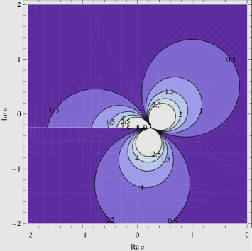
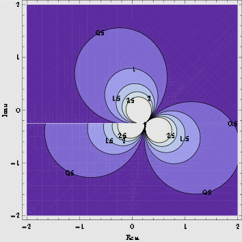
Figure 2: The two different Riemann sheets for rational solutions with broken $\mathcal{PT}$-symmetry of the $\mathcal{H}_{1/3}^{+}$-model with different values of purely complex initial conditions whose imaginary part is indicated in the figure   The asymptotic conditions are chosen to be $\lim_{\zeta\rightarrow\pm\infty}u(\zeta)=(1-i)/4$, the speed of the wave as $c=1$ and the constants of the model as $\beta=2+2i$ and $\gamma=3$

A further characteristic feature of the deformed models is that, in general, one has to view them on various Riemann sheets. An example for a traveling wave solution parameterized by $\zeta=x-ct$, with $c$ denoting the wave speed, for broken $\mathcal{PT}$-symmetry is presented in figure 2.

The branch cut at $-\infty-i/4$ to $(1-i)/4$ is passed from above in panel (a) to below in panel (b). The trajectories for the $\mathcal{PT}$-symmetric and broken $\mathcal{PT}$-symmetric case look qualitatively very similar, the major difference being that the fixed point has moved away from the real axis, thus leading to a loss of the symmetry.

Viewing the systems as two dimensional models, the nature of the fixed points has been investigated systematically by exploiting the fact that their characteristic behaviour is completely classified in dependence on the different types of eigenvalues for the Jacobian. In [18] it was found that they may even undergo Hopf bifurcations in these systems, passing form a star node over a centre to a focus. This feature was derived for the $\mathcal{PT}$-symmetric as well as for the broken $\mathcal{PT}$-symmetric regime. In particular this also means that we encounter closed trajectories despite the fact that the $\mathcal{PT}$-symmetry is broken. We depict an examples in figure 3 for different values of $c$, $\beta$ and $\gamma$.

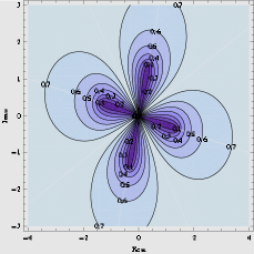
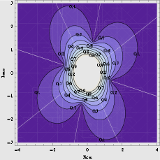
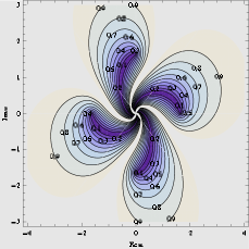
Figure 3: Broken $\mathcal{PT}$-symmetric solution for $\mathcal{H}_{4}^{-}$: (a) Star node at the origin for $c=1$, $\beta=2+i3$, $\gamma=1$; (b) centre at the origin for $c=1$, $\beta=2+i3$, $\gamma=-1$; (c) focus at the origin for $c=1$, $\beta=2$, $\gamma=1+i3$.

An interesting relation between these type of deformations and some simple complex quantum mechanical models was pointed out in [18]. As a special case of this general observation we consider here the model $\mathcal{H}_{2}^{-}$-model with Hamiltonian density

$$\mathcal{H}_{2}^{-}[u]=\frac{\beta}{12}u^{4}+\frac{\gamma}{2}u_{x}^{2},$$ (89)

and make contact with the model studied in [48]. As explained in [18], integrating (87) twice with respect to $\zeta$ we obtain

$$u_{\zeta}^{2}=\frac{2}{\gamma}\left(\kappa_{2}+\kappa_{1}u+\frac{c}{2}u^{2}+\beta\frac{1}{12}u^{4}\right),$$ (90)

with integration constants $\kappa_{1},\kappa_{2}\in\mathbb{C}$. Identifying $u\rightarrow x$ and $\zeta\rightarrow t$ for the traveling wave equation together with the constraints

$$\kappa_{1}=-\gamma\tau,\quad\kappa_{2}=\gamma E_{x},\quad\beta=-3\gamma g\quad\text{and\quad}c=-\gamma\omega^{2},$$ (91)

converts the derivative of equation (90) into Newton’s equation

$$\ddot{x}+\tau+\omega^{2}x+gx^{3}=0,$$ (92)

for the quartic harmonic oscillator of the form

$$H_{\text{quartic}}=E_{x}=\frac{1}{2}p^{2}+\tau x+\frac{\omega^{2}}{2}x^{2}+\frac{g}{4}x^{4}.$$ (93)

One may now directly translate some of the properties of the system (89) to the quantum mechanical model (93). The special choice $\kappa_{1}=\tau=0$ for the integrations constants imply that one is considering asymptotically vanishing waves with $\lim_{\zeta\rightarrow\infty}u(\zeta)=0$ and with Neumann boundary condition $\lim_{\zeta\rightarrow\infty}u_{x}(\zeta)=\sqrt{2E_{x}}$ where $H_{\text{quartic}}=E_{x}$. Accordingly, the energy in the classical analogue of a complex classical particle corresponds to an integration constant in the nonlinear wave equation context multiplied by one of the coupling constants in the latter model. This is of course different from the energy as defined in (88), which also leads to different conclusions regarding the reality of these quantities resulting from the various $\mathcal{PT}$-symmetric scenarios.

In a similar way, the complex seminal [1] cubic harmonic oscillator

$$H_{\text{cubic}}=\frac{1}{2}p^{2}+\frac{1}{2}x^{2}+igx^{3},$$ (94)

treated also in [49] simply results from the integrating the KdV-equation twice with the identification $\kappa_{1}=0$, $\kappa_{2}=\gamma E_{x}$, $\beta=-i6cg$ and $\gamma=-c$.

It appears to be unlikely that the models are still integrable as in general they do not pass the Painlevé test [50, 51]. Similar studies have also be carried out for other types of nonlinear wave equations as for instance for deformed Ito systems in [18]. It was even shown that one can $\mathcal{PT}$-symmetrically deform the supersymmetric version of the KdV-equation (82) while still preserving its supersymmetry [47].

Evidently many features remain still unexplored and it would be very interesting to extend these studies to a larger range of values for the deformation parameter, to other nonlinear field equations such as Burgers, Bussinesque, KP, generalized shallow water equations, extended KdV equations with compacton solution, etc.

Acknowledgments: I would like to thank all my collaborators on the topic presented here for sharing their insights: Paulo Assis, Bijan Bagchi, Olalla Castro-Alvaredo, Andrea Cavaglia, Sanjib Dey, Carla Figueira de Morisson Faria, Laure Gouba, Frederik Scholtz, Monique Smith and Miloslav Znojil.

References

- [1] C. M. Bender and S. Boettcher, Real Spectra in Non-Hermitian Hamiltonians Having PT Symmetry, Phys. Rev. Lett. 80, 5243–5246 (1998).
- [2] F. G. Scholtz, H. B. Geyer, and F. Hahne, Quasi-Hermitian Operators in Quantum Mechanics and the Variational Principle, Ann. Phys. 213, 74–101 (1992).
- [3] C. M. Bender, D. C. Brody, and H. F. Jones, Complex Extension of Quantum Mechanics, Phys. Rev. Lett. 89, 270401(4) (2002).
- [4] A. Mostafazadeh, Pseudo-Hermiticity versus PT symmetry. The necessary condition for the reality of the spectrum, J. Math. Phys. 43, 205–214 (2002).
- [5] C. M. Bender, D. C. Brody, and H. F. Jones, Must a Hamiltonian be Hermitian?, Am. J. Phys. 71, 1095–1102 (2003).
- [6] A. Mostafazadeh and A. Batal, Physical Aspects of Pseudo-Hermitian and -Symmetric Quantum Mechanics, J. Phys. A37, 11645–11680 (2004).
- [7] E. Caliceti, F. Cannata, M. Znojil, and A. Ventura, Construction of PT-asymmetric non-Hermitian Hamiltonians with CPT-symmetry, Phys. Lett. A335, 26–30 (2005).
- [8] C. Figueira de Morisson Faria and A. Fring, Time evolution of non-Hermitian Hamiltonian systems, J. Phys. A39, 9269–9289 (2006).
- [9] F. G. Scholtz and H. B. Geyer, Operator equations and Moyal products – metrics in quasi-hermitian quantum mechanics, Phys. Lett. B634, 84–92 (2006).
- [10] C. Figueira de Morisson Faria and A. Fring, Isospectral Hamiltonians from Moyal products, Czech. J. Phys. 56, 899–908 (2006).
- [11] A. Mostafazadeh, Metric operators for quasi-Hermitian Hamiltonians and symmetries of equivalent Hermitian Hamiltonians, J. Phys. A41, 055304 (2008).
- [12] E. Wigner, Normal form of antiunitary operators, J. Math. Phys. 1, 409–413 (1960).
- [13] J. Dieudonné, Quasi-hermitian operators, Proceedings of the International Symposium on Linear Spaces, Jerusalem 1960, Pergamon, Oxford , 115–122 (1961).
- [14] J. P. Williams, Operators similar to their adjoints, Proc. American. Math. Soc. 20, 121–123 (1969).
- [15] M. Froissart, Covariant formalism of a field with indefinite metric, Il Nuovo Cimento 14, 197–204 (1959).
- [16] E. C. G. Sudarshan, Quantum Mechanical Systems with Indefinite Metric. I, Phys. Rev. 123, 2183–2193 (1961).
- [17] P. Dorey, C. Dunning, and R. Tateo, Spectral equivalences from Bethe ansatz equations, J. Phys. A34, 5679–5704 (2001).
- [18] A. Cavaglia, A. Fring, and B. Bagchi, PT-symmetry breaking in complex nonlinear wave equations and their deformations, J. Phys. A44, 325201 (2011).
- [19] G. von Gehlen, Critical and off-critical conformal analysis of the Ising quantum chain in an imaginary field, J. Phys. A24, 5371–5399 (1991).
- [20] J. L. Cardy, Conformal invariance and the Yang-Lee edge singularity in two-dimension, Phys. Rev. Lett. 54, 1354–1356 (1985).
- [21] A. A. Belavin, A. M. Polyakov, and A. B. Zamolodchikov, Infinite conformal symmetry in two-dimensional quantum field theory, Nucl. Phys. B241, 333–380 (1984).
- [22] O. A. Castro-Alvaredo and A. Fring, A spin chain model with non-Hermitian interaction: The Ising quantum spin chain in an imaginary field, J. Phys. A42, 465211 (2009).
- [23] C. Korff and R. A. Weston, PT Symmetry on the Lattice: The Quantum Group Invariant XXZ Spin-Chain, J. Phys. A40, 8845–8872 (2007).
- [24] T. D. and P. K. G., The exactly solvable quasi-Hermitian transverse Ising model, J. Phys. A42, 475208 (2009).
- [25] C. M. Bender and T. T. Wu, Anharmonic Oscillator, Phys. Rev. 184, 1231–1260 (1969).
- [26] J. von Neuman and E. Wigner, Über merkwürdige diskrete Eigenwerte. Über das Verhalten von Eigenwerten bei adiabatischen Prozessen, Zeit. der Physik 30, 467–470 (1929).
- [27] F. J. Dyson, Thermodynamic Behavior of an Ideal Ferromagnet, Phys. Rev. 102, 1230–1244 (1956).
- [28] A. G. Bytsko, Non-Hermitian spin chains with inhomogeneous coupling, Phys. Rev. B 22N3, 80–106 (2010).
- [29] G. L. Giorgi, Spontaneous symmetry breaking and quantum phase transitions in dimerized spin chains, Phys. Rev. B 82, 052404 (2010).
- [30] A. Fring, A note on the integrability of non-Hermitian extensions of Calogero-Moser-Sutherland models, Mod. Phys. Lett. 21, 691–699 (2006).
- [31] B. Basu-Mallick and B. P. Mandal, On an exactly solvable type Calogero model with nonhermitian PT invariant interaction, Phys. Lett. A284, 231–237 (2001).
- [32] B. Basu-Mallick, T. Bhattacharyya, A. Kundu, and B. P. Mandal, Bound and scattering states of extended Calogero model with an additional PT invariant interaction, Czech. J. Phys. 54, 5–12 (2004).
- [33] B. Basu-Mallick, T. Bhattacharyya, and B. P. Mandal, Phase shift analysis of PT-symmetric nonhermitian extension of Calogero model without confining interaction, Mod. Phys. Lett. A20, 543–552 (2005).
- [34] M. A. Olshanetsky and A. M. Perelomov, Classical integrable finite dimensional systems related to Lie algebras, Phys. Rept. 71, 313–400 (1981).
- [35] H. H. Chen, L. Y. C., and N. R. Pereira, Algebraic internal wave solutions and the integrable Calogero-Moser-Sutherland -body problem, Phys. Fluids 22, 187–188 (1979).
- [36] J. Feinberg, talk at PHHQP workshop VI, City University London, (2007).
- [37] H. Airault, H. P. McKean, and J. Moser, Rational and Elliptic Solutions of the Korteweg-de Vries Equation and a Related Many-Body Problem, Comm. pure appl. Math. 80, 95–148 (1977).
- [38] P. E. G. Assis and A. Fring, From real fields to complex Calogero particles, J. Phys. A42, 425206(14) (2009).
- [39] M. Znojil and M. Tater, Complex Calogero model with real energies, J. Phys. A34, 1793–1803 (2001).
- [40] A. Fring and M. Znojil, -Symmetric deformations of Calogero models, J. Phys. A40, 194010(17) (2008).
- [41] A. Fring and M. Smith, Antilinear deformations of Coxeter groups, an application to Calogero models, J. Phys. A43, 325201 (2010).
- [42] A. Fring and M. Smith, PT invariant complex E(8) root spaces, Int. J. Theor. Phys. 50, 974–981 (2011).
- [43] A. Fring and M. Smith, Non-Hermitian multi-particle systems from complex root spaces, J. Phys. A45, 085203 (2012).
- [44] D. J. Korteweg and deVries G., On the change of form of long waves advancing in a rectangular canal, and on a new type of long stationary waves, Phil. Mag. 39, 422–443 (1895).
- [45] C. M. Bender, D. C. Brody, J. Chen, and E. Furlan, -symmetric extension of the Korteweg-de Vries equation, J. Phys. A40, F153–F160 (2007).
- [46] A. Fring, -Symmetric deformations of the Korteweg-de Vries equation, J. Phys. A40, 4215–4224 (2007).
- [47] B. Bagchi and A. Fring, -symmetric extensions of the supersymmetric Korteweg-De Vries equation, J. Phys. A41, 392004(9) (2008).
- [48] A. G. Anderson, C. M. Bender, and U. I. Morone, Periodic orbits for classical particles having complex energy, Phys. Lett. A375, 3399 3404 (2011).
- [49] C. M. Bender, D. C. Brody, and D. W. Hook, Quantum effects in classical systems having complex energy, J. Phys. A41, 352003 (2008).
- [50] P. E. G. Assis and A. Fring, Integrable models from -symmetric deformations, J. Phys. A42, 105206 (2009).
- [51] P. E. G. Assis and A. Fring, Compactons versus Solitons, Pramana J. Phys. 74, 857–865 (2010).