Asymptotic behaviour of zeros of exceptional Jacobi and Laguerre polynomials

Abstract.

The location and asymptotic behaviour for large $n$ of the zeros of exceptional Jacobi and Laguerre polynomials are discussed. The zeros of exceptional polynomials fall into two classes: the regular zeros, which lie in the interval of orthogonality and the exceptional zeros, which lie outside that interval. We show that the regular zeros have two interlacing properties: one is the natural interlacing between consecutive polynomials as a consequence of their Sturm-Liouville character, while the other one shows interlacing between the zeros of exceptional and classical polynomials. A generalization of the classical Heine-Mehler formula is provided for the exceptional polynomials, which allows to derive the asymptotic behaviour of their regular zeros. We also describe the location and the asymptotic behaviour of the exceptional zeros, which converge for large $n$ to fixed values.

1. Introduction

Let $\mu$ be a probability measure supported on an infinite subset $E$ of the real line. We assume that $\int_{E}|x^{n}|d\mu<\infty$ for every nonnegative number $n$. A sequence of monic polynomials $\{P_{n}(x)\}_{n\geq 0}$ is said to be orthogonal with respect to $\mu$ when deg $P_{n}=n$ and $\int_{E}P_{n}(x)P_{m}(x)d\mu(x)=0$ for $n\neq m$. It is very well known that these polynomials satisfy a three term recurrence relation that yields for the orthonormalized polynomials a symmetric tridiagonal (Jacobi) matrix such that the eigenvalues of the $n$ leading principal submatrix are the zeros of the polynomial $P_{n}$. As a straightforward consequence of this fact the zeros of $P_{n}$ are real, simple and interlace with the zeros of $P_{n-1}$. On the other hand, they are located in the interior of the convex hull of $E$.

The theory of orthogonal polynomials is strongly related to Sturm-Liouville problems. In particular, the so called classical orthogonal polynomials (Hermite, Laguerre, and Jacobi) appear as eigenfunctions of second order linear differential operators with polynomial coefficients. Indeed, the corresponding measure of orthogonality is absolutely continuous and their derivative with respect to the Lebesgue measure (weight function) is the density function of the normal, gamma and beta distributions, respectively. Notice that this fact was pointed out by E. Routh in 1884 [41] as well as by S. Bochner in 1929 [2], but the orthogonality does not play therein any role. On the other hand, they are hypergeometric functions and, as a consequence, many analytic properties can be deduced from this fact. Moreover, certain properties of their zeros can be easily deduced using the classical Sturm theorems. Finally, a nice electrostatic interpretation of their zeros is deduced from the second order linear differential equation as an equilibrium problem for the logarithmic interaction of positive unit charges under an external field.

Exceptional orthogonal polynomials constitute a recent new approach to spectral problems for second order linear differential operators with polynomial eigenfunctions. Previously, a constructive theory of orthogonal polynomials related to the classical ones has been done in two directions. The first one is related to the spectral theory of higher order linear differential operators with polynomial coefficients. For fourth order differential operators the classification of their eigenfunctions, which are sequences of orthogonal polynomials with respect to a nontrivial probability measure supported on an infinite subset of the real line, was done by H. L. Krall and A. M. Krall [27, 28, 29] and essentially yields the classical ones and perturbations of some particular Laguerre weights ${\rm e}^{-x}+M\delta(x)$, Jacobi weights $(1-x)^{\alpha}+M\delta(x)$ and Legendre weight $1+M\delta(x-1)+M\delta(x+1)$, $M\geq 0$. For higher order, some examples are known but a general theory and classification constitutes an open problem. The second one appears when some perturbations of the measure are considered. In particular, three cases are considered in the literature in the framework of the so called spectral linear transformations [45]. The Christoffel transformation (the multiplication of the measure by a positive polynomial in the support of the measure), the Uvarov transformation (the addition of mass points off the support of the measure) and Geronimus transformation (the multiplication by the inverse of a positive polynomial). They can be analyzed in terms of the discrete Darboux transformation of the corresponding Jacobi matrices using the LU and UL factorizations and commuting them [3].

Exceptional orthogonal polynomials depart from the classical families in that the sequence of exceptional polynomials is not required to contain a polynomial of every degree, and as a consequence new differential operators exist, with rational rather than polynomial coefficients. Despite this fact, the sequence of exceptional polynomial eigenfunctions is still dense in the corresponding weighted $L^{2}$ space and constitutes an orthogonal polynomial system. The measure of orthogonality for the exceptional families is a classical measure divided by the square of a polynomial with zeros outside the support of the measure.

The first explicit examples of families of exceptional orthogonal polynomials are the $\mathrm{X}_{1}$-Jacobi and $\mathrm{X}_{1}$-Laguerre polynomials, which are of codimension one, and were first introduced in [15, 16]. In these papers, a characterization theorem was proved for these orthogonal polynomial families, realizing them as the unique complete codimension one families defined by a Sturm-Liouville problem. One of the key steps in the proof was the determination of normal forms for the flags of univariate polynomials of codimension one in the space of all such polynomials, and the determination of the second-order linear differential operators which preserve these flags [13, 19].

Shortly after, Quesne [33, 34] observed the presence of a relationship between exceptional orthogonal polynomials and the Darboux transformation. This enabled her to obtain examples of potentials corresponding to orthogonal polynomial families of codimension two, as well as explicit families of $\mathrm{X}_{2}$ polynomials. Higher-codimensional families were first obtained by Odake and Sasaki [36]. The same authors further showed the existence of two families of $\mathrm{X}_{m}$-Laguerre and $\mathrm{X}_{m}$-Jacobi polynomials [37], the existence of which was explained in [17] for $\mathrm{X}_{m}$-Laguerre polynomials and in [19] for $\mathrm{X}_{m}$-Jacobi polynomials, through the application of the isospectral algebraic Darboux transformation first introduced in [11, 12]. These exceptional orthogonal polynomials have been applied in a number of interesting physical contexts, such as Dirac operators minimally coupled to external fields, [24], entropy measures in quantum information theory, [9], rational extensions of Morse and Kepler-Coulomb problems, [21, 22] or discrete quantum mechanics, [40].

The aim of our contribution is to explore analytic properties of these exceptional polynomials. In particular we will focus our attention in the distribution of their zeros in terms of the support of the orthogonality measure as well as their limit behavior. On the other hand, we will analyze some asymptotic properties as the outer relative asymptotics in terms of the corresponding classical orthogonal polynomials and the Mehler-Heine type formulas. Some properties of the zeros have also been analyzed numerically in [25].

2. Exceptional orthogonal polynomials

Let $W(z)$ be a positive weight function with finite moments. Usually, orthogonal polynomials are defined by applying Gram-Schmidt orthogonalization to the standard flag $1,z,z^{2},\ldots$ relative to an $L^{2}$ inner product associated with the weight $W$. Moreover, if the resulting orthogonal polynomials are eigenfunctions of a Sturm-Liouville problem, we speak of classical orthogonal polynomials. By Bochner’s theorem, the range of such polynomials is limited to the classical families of Hermite, Laguerre, and Jacobi (for positive weights) and Bessel (for signed weights).

In order to go beyond the classical families, we consider orthogonal polynomials spanning a non-standard polynomial flag, say with a basis $p_{m}(z),p_{m+1}(z),\ldots,$ where $\deg p_{j}=j$. Once we drop the assumption that the OP sequence contains a polynomial of every degree, we obtain new classes of orthogonal polynomials defined by Sturm-Liouville problems, which are commonly referred to as exceptional orthogonal polynomials (XOPs).

In the last two years it has become clear that the Darboux transformation, appropriately generalized to the polynomial context, plays an essential part in the deliniation of XOPs. To wit, let $\mathcal{P}_{n}$ denote the vector space of polynomials of degree $\leq n$, and consider a codimension $m$ polynomial flag

$$\mathcal{U}=\{U_{k}\}_{k=1}^{\infty},\quad U_{k-1}\subset U_{k}\subset\mathcal{P}_{m+k-1}\,.$$

Furthermore, let

(1) $$A[y]=b(z)(y^{\prime}-w(z)y),\quad B[y]=\hat{b}(z)(y^{\prime}-\hat{w}(z)y)$$

be first order linear differential operators with rational coefficients such that

(2) $$B[\mathcal{P}_{k-1}]=U_{k},\quad A[U_{k}]=\mathcal{P}_{k-1},\qquad k=1,2,\dots$$

i.e. $B$ maps the standard flag into the codimension $m$ flag while $A$ maps the codimension $m$ into the standard flag. Note that equation (2) implies that $\ker A=\ker B=0$ and the Darboux transformation is isospectral. Next, consider the second order differential operators

(3) $$T=AB,\quad\hat{T}=BA.$$

By construction, $T$ leaves invariant the standard polynomial flag, while $\hat{T}$ leaves invariant the codimension-$m$ flag $\mathcal{U}$. Hence, by Bochner’s theorem,

(4) $$T[y]=p(z)y^{\prime\prime}+q(z)y^{\prime}+r(z)y,\quad\hat{T}[y]=p(z)y^{\prime\prime}+\hat{q}(z)y^{\prime}+\hat{r}(z)y$$

where $p,q,r$ are polynomials with $\deg p\leq 2,\deg q\leq 1,\deg r=0$ but where $\hat{q},\hat{r}$ are in general rational functions. It is then assured that $T$ and $\hat{T}$ have polynomial eigenfunctions . Let $y_{j},\;j\geq 0$, denote the polynomial eigenfunctions of $T[y]$ and $\hat{y}_{j},\;j\geq m$, denote the polynomial eigenfunctions of $\hat{T}[y]$. Again, by construction we have the following intertwining relations

(5) $$TA=A\hat{T},\quad BT=\hat{T}B,$$

which mean that

(6) $$B[y_{j}]=\beta_{j}\hat{y}_{j+m},\quad A[\hat{y}_{j+m}]=\alpha_{j}y_{j},\quad j=0,1,2,\ldots,$$

where $\alpha_{j},\beta_{j}$ are constants, i.e. operator $A$ maps eigenfunctions of $T$ into eigenfunctions of $\hat{T}$ while $B$ does the opposite transformation.

Furthermore, let

(7) $$W(z)=\frac{1}{p}\exp\int^{z}\!\!\frac{q}{p},\qquad\hat{W}=\frac{1}{p}\exp\int^{z}\!\!\frac{\hat{q}}{p}$$

be the solutions of the Pearson’s equations

(8) $$(pW)^{\prime}=qW,\quad(p\hat{W})^{\prime}=\hat{q}\hat{W}.$$

This means that $T[y]$ is formally self-adjoint relative to $W$ while $\hat{T}[y]$ is formally self-adjoint relative to $\hat{W}$. Consequently, the eigenpolynomials $y_{j}$ are formally orthogonal with respect to the weight $W(z)$, while $\hat{y}_{j}$ are formally orthogonal relative to $\hat{W}(z)$. One can also show that

$$\int A[f]gWdz+\int B[g]f\hat{W}dz=\text{ boundary term};$$

which means that operators $A$ and $-B$ are formally adjoint. By a careful choice of the flags, and by imposing appropriate boundary conditions one can construct examples where the above formal relations hold in the $L^{2}$ setting (i.e. boundary conditions such that the boundary terms vanish) and thereby obtain novel classes of exceptional orthogonal polynomials.

In the present note we study asymptotic behaviour of XOPs of Laguerre and Jacobi types. As we show, in the interval of orthogonality the exceptional polynomials satisfy a variant of the classical Heine-Mehler formula. Outside the interval of orthogonality, the convergence picture is less clear. However, one can show that codimension $m$ exceptional orthogonal polynomials possess $m$ extra zeros outside the interval of orthogonality, which we shall denote as exceptional zeros. These exceptional zeros have well-defined convergence behaviour, and they converge to the zeros of some fixed classical orthogonal polynomial.

3. Type I Exceptional Laguerre polynomials

Let us illustrate the above discussion with the particular example of the so-called type I exceptional Laguerre polynomials. Let $L_{n}^{{({\alpha})}}(z)$ denote the classical Laguerre polynomial of degree $n$ and

$$\mathcal{L}_{\alpha}[y]=zy^{\prime\prime}+({\alpha}+1-z)y^{\prime}$$

the classical Laguerre operator. Thus, $y=L_{n}^{{({\alpha})}}$ is the unique polynomial solution of the equation

$$\mathcal{L}_{\alpha}[y]=-ny,\quad\text{ with the normalization }\quad y^{(n)}(0)=(-1)^{n}.$$

An equivalent boundary condition is

(9) $$L_{n}^{{({\alpha})}}(0)=\binom{n+{\alpha}}{n}.$$

For a fixed non-negative integer $m\geq 0$, let us now define

(10) $$\xi_{{\alpha},m}(z) =L_{m}^{{({\alpha})}}(-z),$$

(11) $$A^{{\rm{I}}}_{{\alpha},m}[y] =\xi_{{\alpha},m}y^{\prime}-\xi_{{\alpha}+1,m}y,$$

(12) $$B^{{\rm{I}}}_{{\alpha},m}[y] =\frac{zy^{\prime}+(1+{\alpha})\,y}{\xi_{{\alpha},m}},$$

(13) $$L_{m,m+j}^{{\rm{I}}({\alpha})} =-A^{{\rm{I}}}_{{\alpha}-1,m}\left[L_{j}^{{({\alpha}-1)}}\right],\qquad j=0,1,2,\dots$$

(14) $$\mathcal{L}^{{\rm{I}}}_{{\alpha},m}[y] =\mathcal{L}_{\alpha}[y]+my-2(\log\xi_{{\alpha}-1,m})^{\prime}\left(zy^{\prime}+{\alpha}y\right).$$

The following factorization relations follow from standard Laguerre identities:

(15) $$\mathcal{L}_{{\alpha}} =B^{{\rm{I}}}_{{\alpha},m}A^{{\rm{I}}}_{{\alpha},m}+{\alpha}+m+1,$$

(16) $$\mathcal{L}^{{\rm{I}}}_{{\alpha},m} =A^{{\rm{I}}}_{{\alpha}-1,m}B^{{\rm{I}}}_{{\alpha}-1,m}+{\alpha}+m.$$

Consider now the following codimension $m$ polynomial subspace

(17) $$U^{\rm{I}}_{{\alpha},j}=\{f\in\mathcal{P}_{j+m-1}:\xi_{{\alpha}-1,m}|(zf^{\prime}+{\alpha}f)\},\qquad j=1,2,\ldots,$$

where $f|g$ means polynomial $f(z)$ divides polynomial $g(z)$. At the level of flags, the above factorizations correspond to the following linear isomorphisms:

(18) $$B^{\rm{I}}_{{\alpha}-1,m}:U^{\rm{I}}_{{\alpha},j}\to\mathcal{P}_{j-1},\qquad A^{\rm{I}}_{{\alpha}-1,m}:\mathcal{P}_{j-1}\to U^{\rm{I}}_{{\alpha},j}.$$

The polynomials $\left\{L_{m,m+j}^{{\rm{I}}({\alpha})}\right\}_{j=0}^{\infty}$ are known in the literature as the type I exceptional codimension $m$ Laguerre polynomials (for short, type I $X_{m}$-Laguerre) [36, 17]. By construction, the $X_{m}$-Laguerre polynomials have the following properties:

• they span the flag $U^{\rm{I}}_{{\alpha},1}\subset U^{\rm{I}}_{{\alpha},2}\subset\cdots$

• they satisfy the following second order linear differential equation:

  (19) $$\mathcal{L}^{\rm{I}}_{{\alpha},m}\left[L_{m,m+j}^{{\rm{I}}({\alpha})}\right]=-jL_{m,m+j}^{{\rm{I}}({\alpha})},\qquad j\geq 0,$$

• they are orthogonal with respect to the weight

  (20) $$W^{{\rm{I}}}_{{\alpha},m}(z):=\frac{z^{\alpha}e^{-z}}{\xi_{\alpha-1,m}(z)^{2}}=\frac{z^{\alpha}e^{-z}}{\left[L_{m}^{{({\alpha}-1)}}(-z)\right]^{2}},\quad z\in[0,\infty),$$

• they are dense in the Hilbert space $\mathrm{L}^{2}\big{(}[0,\infty),W^{{\rm{I}}}_{{\alpha},m}\big{)}$.

Note that for ${\alpha}\geq 0$ the polynomial $\xi_{{\alpha}-1,m}(z)=L_{m}^{{({\alpha}-1)}}(-z)$ in the denominator of the weight has its zeros on the negative real axis, and hence $W^{\rm{I}}_{{\alpha},m}dz$ is a positive definite measure in $\mathbb{R}^{+}$, with well defined moments of all orders. As a result, for ${\alpha}\geq 0$ the set $\{L_{m,n}^{{\rm{I}}({\alpha})}\}_{n=m}^{\infty}$ constitutes an orthogonal polynomial basis of $\mathrm{L}^{2}\big{(}[0,\infty),W^{{\rm{I}}}_{{\alpha},m}\big{)}$. We observe that the last property of the above list does not follow by the algebraic construction and needs to be established by a separate argument. The interested reader is referred to [17] for a direct proof of the completeness of the $X_{m}$-Laguerre families.

Proposition 3.1.

The type I $X_{m}$-Laguerre polynomials $L_{m,n}^{{\rm{I}}({\alpha})}$ can be expressed in terms of classical associated Laguerre polynomials with the same parameter ${\alpha}$ as follows

(21) $$L_{m,m+j}^{{\rm{I}}({\alpha})}=\xi_{{\alpha},m}L_{j}^{{({\alpha})}}-\xi_{{\alpha},m-1}L_{j-1}^{{({\alpha})}},\qquad j\geq 0.$$

The above representation will be specially useful to discuss the asymptotic properties of the zeros of type I $X_{m}$-Laguerre polynomials. It is clear from it that $L_{m,m+j}^{{\rm{I}}({\alpha})}$ has degree $m+j$. This representation is reminiscent of the expansions obtained by rational modifications of classical weights in the framework of spectral linear transformations (see [45]). However, it should be stressed that they are essentially different because in the case of exceptional polynomials, although there is a rational modification of the weight, we are not dealing with the standard flag.

Proof.

Using elementary identities, we have

$$0 =\xi_{{\alpha},m}(L_{j}^{{({\alpha})}}-L_{j-1}^{{({\alpha})}}-L_{j}^{{({\alpha}-1)}})+L_{j-1}^{{({\alpha})}}(\xi_{{\alpha},m}-\xi_{{\alpha},m-1}-\xi_{{\alpha}-1,m})$$

$$=-(\xi_{{\alpha},m}L_{j}^{{({\alpha}-1)}}+\xi_{{\alpha}-1,m}L_{j-1}^{{({\alpha})}})+(\xi_{{\alpha},m}L_{j}^{{({\alpha})}}-\xi_{{\alpha},m-1}L_{j-1}^{{({\alpha})}}).$$

Therefore, we can re-express the type I $X_{m}$-Laguerre polynomials as

$$L_{m,m+j}^{{\rm{I}}({\alpha})} =\xi_{{\alpha},m}L_{j}^{{({\alpha}-1)}}-\xi_{{\alpha}-1,m}{L_{j}^{{({\alpha}-1)}}}^{\prime}$$

$$=\xi_{{\alpha},m}L_{j}^{{({\alpha}-1)}}+\xi_{{\alpha}-1,m}L_{j-1}^{{({\alpha})}}$$

$$=\xi_{{\alpha},m}L_{j}^{{({\alpha})}}-\xi_{{\alpha},m-1}L_{j-1}^{{({\alpha})}}.$$

∎

We are now ready to prove an interlacing result for the zeros of type I $X_{m}$-Laguerre polynomials, but before let us recall the following classical identity

(22) $$L_{n}^{{({\alpha})}}(0)=({\alpha}+1)_{n}/n!$$

where

$$(x)_{n}=\begin{cases}x(x+1)\cdots(x+n-1)&\text{if $n\geq 0$,}\\ 1&\text{if $n=0$,}\end{cases}$$

is the usual Pochhammer symbol. Using the above representation we obtain an analogous expression for the type I $X_{m}$-Laguerre polynomials:

(23) $$L_{m,m+j}^{{\rm{I}}({\alpha})}(0)=\frac{{\alpha}+j+m}{k}\frac{({\alpha})_{m}}{m!}\frac{({\alpha})_{j}}{j!}$$

Proposition 3.2.

For ${\alpha}>0$ the type I exceptional Laguerre polynomial $L_{m,m+j}^{{\rm{I}}({\alpha})}(z)$ has $j$ simple zeros in $z\in(0,\infty)$ and $m$ simple zeros in $z\in(-\infty,0)$. The positive zeros of $L_{m,m+j}^{{\rm{I}}({\alpha})}(z)$ are located between consecutive zeros of $L_{j}^{{({\alpha})}}$ and $L_{j-1}^{{({\alpha})}}$ with the smallest positive zero of $L_{m,m+j}^{{\rm{I}}({\alpha})}(z)$ located to the left of the smallest zero of $L_{j}^{{({\alpha})}}$. The negative zeros of $L_{m,m+j}^{{\rm{I}}({\alpha})}(z)$ are located between the consecutive zeros of $\xi_{{\alpha},m-1}$ and $\xi_{{\alpha},m}$.

Proof.

Let $0<\zeta_{n,1}^{{\alpha}}<\zeta_{n,2}^{{\alpha}}<\cdots<\zeta_{n,n}^{{\alpha}}$ denote the zeros of $L_{n}^{{({\alpha})}}(z)$ listed in increasing order. According to the interlacing property of the zeros of classical orthogonal polynomials, we have

$$\zeta_{j,1}^{{\alpha}}<\zeta_{j-1,1}^{{\alpha}}<\zeta_{j,2}^{{\alpha}}<\zeta_{j-1,2}^{{\alpha}}<\cdots<\zeta_{j-1,j-1}^{{\alpha}}<\zeta_{j,j}^{{\alpha}}.$$

Recall that $L_{n}^{{({\alpha})}}(z)>0$ for $z\leq 0$. This implies that $\xi_{{\alpha},m}(z),\xi_{{\alpha},m-1}(z)>0$ for $z\geq 0$. Hence, by (21),

$$\operatorname{sgn}L_{m,m+j}^{{\rm{I}}({\alpha})}(\zeta_{j,i}^{{\alpha}})=(-1)^{i},\quad i=1,\ldots,j;$$

$$\operatorname{sgn}L_{m,m+j}^{{\rm{I}}({\alpha})}(\zeta_{j-1,i}^{{\alpha}})=(-1)^{i},\quad i=1,\ldots,j-1.$$

It follows by (23) that there is a zero of $L_{m,m+j}^{{\rm{I}}({\alpha})}$ in the interval $(0,\zeta_{j,1}^{{\alpha}})$ and a zero in the interval $(\zeta_{j-1,i-1}^{{\alpha}},\zeta_{j,i}^{{\alpha}})$ for every $i=2,\ldots,j$. An analogous argument places zeros of $L_{m,m+j}^{{\rm{I}}({\alpha})}$ in the intervals $(-\zeta_{m,1}^{{\alpha}},0)$ and $(-\zeta_{m,i}^{{\alpha}},-\zeta_{m-1,i-1}^{{\alpha}}),\;i=2,\ldots,m$. By exhaustion, each of the above intervals contains one simple zero of $L_{m,m+j}^{{\rm{I}}({\alpha})}$. ∎

We now study the distribution of the zeros of $L_{m,n}^{{\rm{I}}({\alpha})}$ as $n\to\infty$. To that end, we will use the classical Heine-Mehler formula for Laguerre polynomials

(24) $$L_{n}^{{({\alpha})}}\left(z/n\right)n^{-{\alpha}}\rightrightarrows z^{-{\alpha}/2}J_{{\alpha}}(2\sqrt{z}),\qquad n\to\infty,$$

where $J_{\alpha}(z)$ denotes the Bessel function of the first kind of order ${\alpha}$ $({\alpha}>-1)$ and the double arrow denotes uniform convergence in compact domains of the complex plane.

The exceptional Laguerre polynomials admit a generalization of the classical Heine-Mehler formula, given by the following:

Proposition 3.3 (Generalized Heine-Mehler formula).

We have

(25) $$L_{m,n}^{{\rm{I}}({\alpha})}\left(z/n\right)n^{-{\alpha}}\rightrightarrows\binom{{\alpha}+m-1}{m}z^{-{\alpha}/2}J_{\alpha}(2\sqrt{z}),\qquad n\to\infty.$$

A numerical representation of the convergence of the scaled exceptional Laguerre polynomials to the Bessel function is given in Figure 1.

Proof.

Multiply (21) by $j^{-{\alpha}}$ and replace $z\to z/j$. Taking the limit $j\to\infty$ and using the classical Heine-Mehler formula (24) leads to

$$j^{-{\alpha}}L_{m,m+j}^{{\rm{I}}({\alpha})}\rightrightarrows\big{(}\xi_{{\alpha},m}(0)-\xi_{{\alpha},m-1}(0)\big{)}z^{-{\alpha}/2}J_{\alpha}(2\sqrt{z}).$$

The final expression (25) is recovered by noting that

$$\xi_{{\alpha},m}(0)-\xi_{{\alpha},m-1}(0)=\binom{{\alpha}+m-1}{m}$$

as implied by (10) and (22). ∎

Note that for $m=0$ the classical Heine-Mehler formula is recovered as a particular case.

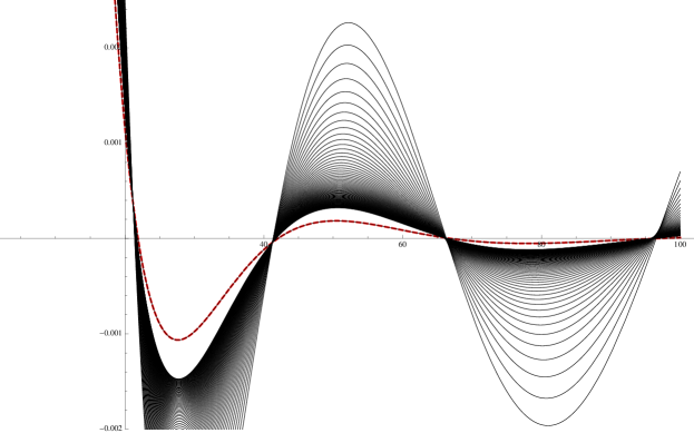
Figure 1. Plot of $n^{-{\alpha}}L_{m,{\alpha}}^{{\rm{I}}(n)}(x/n)$ for $m=3$, ${\alpha}=5.5$ and $20\leq n\leq 100$. The dashed red line corresponds to the limiting Bessel function $x^{-{\alpha}/2}\binom{{\alpha}+m-1}{m}J_{\alpha}(2\sqrt{x})$ predicted by the generalized Heine-Mehler formula (25).

Corollary 3.1.

Let $\left\{\tilde{z}^{({\alpha})}_{i}\right\}_{i\geq 1}$ be the sequence of zeros of the Bessel function $J_{\alpha}(z)$ listed in increasing order and let $\{x_{j,i}\}_{i=1}^{j}$ denote the regular zeros of $L_{m,m+j}^{{\rm{I}}({\alpha})}(z)$ in the interval $[0,\infty)$. Then we get the following asymptotic behaviour

(26) $$\lim_{j\to\infty}jx_{j,i}=\frac{(\tilde{z}^{({\alpha})}_{i})^{2}}{4}.$$

Proof.

The above result follows from (25) and Hurwitz’s theorem. ∎

We have already seen that for fixed $m$ the asymptotic behaviour of the regular zeros of the exceptional Laguerre polynomials coincides with that of the classical Laguerre. We now investigate in the same limit the behaviour of the $m$ exceptional zeros of $L_{m,m+j}^{{\rm{I}}({\alpha})}(z)$.

Proposition 3.4.

As $j\to\infty$ the $m$ zeros of $L_{m,m+j}^{{\rm{I}}(k)}$ in $(-\infty,0)$ converge to the $m$ zeros of $L_{m}^{{({\alpha}-1)}}(-z)$.

Proof.

The classical Laguerre polynomials have the following outer ratio asymptotics

(27) $$\frac{L_{n+1}^{{({\alpha})}}(z)}{L_{n}^{{({\alpha})}}(z)}\rightrightarrows 1,\qquad z\notin[0,\infty),\qquad n\to\infty.$$

Hence, by (21), we have for $z\notin[0,\infty)$,

$$\frac{L_{m,m+j}^{{\rm{I}}({\alpha})}}{L_{j}^{{({\alpha})}}}=\xi_{{\alpha},m}-\xi_{{\alpha},m-1}\frac{L_{j-1}^{{({\alpha})}}}{L_{j}^{{({\alpha})}}}\rightrightarrows\xi_{{\alpha},m}-\xi_{{\alpha},m-1}=\xi_{{\alpha}-1,m}.$$

Therefore, by Hurwitz’s theorem the $m$ exceptional zeros of $L_{m,m+j}^{{\rm{I}}({\alpha})}$ converge to the zeros of $\xi_{{\alpha}-1,m}=L_{m}^{{({\alpha}-1)}}(-z)$. ∎

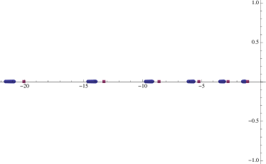
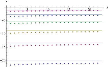
Figure 2. Left: Exceptional zeros of the polynomials $L_{m,m+j}^{{\rm{I}}({\alpha})}(z)$ for $m=6$, ${\alpha}=3.5$ and $1\leq j\leq 22$. The squares denote the zeros of $L_{m}^{{({\alpha}-1)}}(-z)$ to which the zeros of $L_{m,m+j}^{{\rm{I}}({\alpha})}(z)$ converge for $j\to\infty$. Right: Convergence is better seen by plotting the position of the negative zeros as a function of $j$. Solid lines show the limiting values.

4. Type II Exceptional Laguerre polynomials

4.1. Definition and identities.

Let $m\geq 0$ be an integer and ${\alpha}$ a real number. Let us introduce the polynomials

(28) $$\eta_{{\alpha},m}(z):=L_{m}^{{(-{\alpha})}}(z).$$

For a fixed non-negative integer $m$ and a real number $\alpha$ let us define the following first and second order operators

(29) $$A^{\rm{II}}_{{\alpha},m}[y] :=z\eta_{{\alpha},m}y^{\prime}+({\alpha}-m)\eta_{{\alpha}+1,m}y,$$

(30) $$B^{\rm{II}}_{{\alpha},m}[y] :=(y^{\prime}-y)/\eta_{{\alpha},m},$$

(31) $$\mathcal{L}[y] :=zy^{\prime\prime}+({\alpha}+1-z)y^{\prime},$$

(32) $$\mathcal{L}^{\rm{II}}_{{\alpha},m}[y] :=\mathcal{L}[y]+2z(\log\eta_{{\alpha}+1,m})^{\prime}(y-y^{\prime})-my.$$

The following factorizations follow from standard Laguerre identities:

(33) $$\mathcal{L}_{\alpha} =B^{\rm{II}}_{{\alpha},m}A^{\rm{II}}_{{\alpha},m}+{\alpha}-m,$$

(34) $$\mathcal{L}^{\rm{II}}_{{\alpha},m} =A^{\rm{II}}_{{\alpha}+1,m}B^{\rm{II}}_{{\alpha}+1,m}+{\alpha}+1-m.$$

For a real number $\alpha$ and given integers $n\geq m\geq 0$, we define the $n^{\text{th}}$ degree type II exceptional Laguerre polynomial by

(35) $$L_{m,n}^{{\rm{II}}({\alpha})}(z) :=-A^{\rm{II}}_{\alpha+1,m}[L_{j}^{{({\alpha}+1)}}],\qquad j=n-m\geq 0.$$

Expanding (29) and applying standard identities, the following dual representations of the type II polynomials hold:

(36) $$L_{m,m+j}^{{\rm{II}}({\alpha})} =zL_{m}^{{(-{\alpha}-1)}}L_{j-1}^{{({\alpha}+2)}}+(m-{\alpha}-1)L_{m}^{{(-{\alpha}-2)}}L_{j}^{{({\alpha}+1)}}$$

(37) $$=-zL_{m-1}^{{(-{\alpha})}}L_{j}^{{({\alpha}+1)}}-({\alpha}+1+j)L_{m}^{{(-{\alpha}-1)}}L_{j}^{{({\alpha})}}.$$

Hence, up to a constant factor, the type II polynomials extend their classical counterparts, which are recovered for the particular case $m=0$:

(38) $$L_{0,n}^{{\rm{II}}({\alpha})}=-(1+{\alpha}+n)L_{n}^{{({\alpha})}}.$$

The factorizations (33) and (34) yield the following intertwining relations between the standard Laguerre operator $\mathcal{L}_{\alpha}$ and the type II $X$-Laguerre operator $\mathcal{L}^{\rm{II}}_{{\alpha},m}$:

(39) $$\mathcal{L}^{\rm{II}}_{{\alpha},m}A^{\rm{II}}_{{\alpha}+1,m}=A^{\rm{II}}_{{\alpha}+1,m}\mathcal{L}_{{\alpha}+1},$$

(40) $$B^{\rm{II}}_{{\alpha}+1,m}\mathcal{L}^{\rm{II}}_{{\alpha},m}=\mathcal{L}_{{\alpha}+1}B^{\rm{II}}_{{\alpha}+1,m}.$$

The former relation provides the eigenvalue relation for the type II exceptional Laguerre polynomials:

(41) $$\mathcal{L}^{\rm{II}}_{{\alpha},m}\left[L_{m,m+j}^{{\rm{II}}({\alpha})}\right]=-jL_{m,m+j}^{{\rm{II}}({\alpha})},\qquad j=0,1,2\dots.$$

The latter gives the following “lowering” relation between the type II exceptional Laguerre polynomials and their classical counterparts:

(42) $$L_{m,n}^{{\rm{II}}({\alpha})}\,{}^{\prime}-L_{m,n}^{{\rm{II}}({\alpha})}=(1+n-{\alpha})L_{m}^{{(-{\alpha}-1)}}L_{j}^{{({\alpha}+1)}},\quad j=n-m\geq 0$$

In order to find raising and lowering relations for the exceptional Laguerre polynomials, let us introduce the following first order linear differential operators

(43) $${\hat{A}}^{\rm{II}}_{{\alpha},m}[y] :=\frac{\eta_{{\alpha}+2,m}}{\eta_{{\alpha}+1,m}}\left(y^{\prime}-(\log\eta_{{\alpha}+2,m})^{\prime}y\right),$$

(44) $${\hat{B}}^{\rm{II}}_{{\alpha},m}[y] :=\frac{\eta_{{\alpha}+1,m}}{\eta_{{\alpha}+2,m}}\left(zy^{\prime}+({\alpha}+1-z)y\right)-z(\log\eta_{{\alpha}+2,m})^{\prime}y.$$

In terms of these operators we have the following shape-invariant factorizations

(45) $$\mathcal{L}^{\rm{II}}_{{\alpha},m} ={\hat{B}}^{\rm{II}}_{{\alpha},m}{\hat{A}}^{\rm{II}}_{{\alpha},m},$$

(46) $$\mathcal{L}^{\rm{II}}_{{\alpha}+1,m} ={\hat{A}}^{\rm{II}}_{{\alpha},m}{\hat{B}}^{\rm{II}}_{{\alpha},m}+1.$$

From these factorizations the following lowering and raising relations for the exceptional polynomials easily follow:

(47) $${\hat{A}}^{\rm{II}}_{{\alpha},m}\left[L_{m,n}^{{\rm{II}}({\alpha})}\right]=L_{m,n-1}^{{\rm{II}}({\alpha}+1)},\quad n\geq m+1,$$

(48) $${\hat{B}}^{\rm{II}}_{{\alpha},m}\left[L_{m,n}^{{\rm{II}}({\alpha}+1)}\right]=(n-m)L_{m,n+1}^{{\rm{II}}({\alpha})},\quad n\geq m.$$

The above equations can be conveniently re-written as

(49) $$\left(\frac{L_{m,n}^{{\rm{II}}({\alpha})}}{\eta_{{\alpha}+2,m}}\right)^{\prime}=\left(\frac{\eta_{{\alpha}+1,m}}{\eta_{{\alpha}+2,m}}\right)^{2}\frac{L_{m,n-1}^{{\rm{II}}({\alpha}+1)}}{\eta_{{\alpha}+1,m}}\,,$$

(50) $$\left(\frac{e^{-z}z^{{\alpha}+1}}{\eta_{{\alpha}+1,m}}L_{m,n}^{{\rm{II}}({\alpha}+1)}\right)^{\prime}=(n-m+1)\left(\frac{\eta_{{\alpha}+2,m}}{\eta_{{\alpha}+1,m}}\right)^{2}\frac{e^{-z}z^{{\alpha}}}{\eta_{{\alpha}+2,m}}L_{m,n+1}^{{\rm{II}}({\alpha})}\,.$$

4.2. Orthogonality

The type II exceptional Laguerre polynomials are formally orthogonal with respect to the weight

(51) $$W^{\rm{II}}_{{\alpha},m}(z):=\frac{e^{-z}z^{\alpha}}{\eta_{{\alpha}+1,m}^{2}}=\frac{e^{-z}z^{\alpha}}{\left[L_{m}^{{(-{\alpha}-1)}}(z)\right]^{2}}.$$

The above weight is the solution $W^{\rm{II}}={\hat{W}}$ of Pearson’s equation (8) where

$$p=z,\quad\hat{q}=(1+{\alpha}-z)-2z(\log\eta_{{\alpha}+1,m})^{\prime}$$

are extracted from (32). As a consequence, (41) and Green’s formula imply

(52) $$(n_{2}-n_{1})\int L_{m,n_{2}}^{{\rm{II}}({\alpha})}\,L_{m,n_{1}}^{{\rm{II}}({\alpha})}\,W^{\rm{II}}_{{\alpha},m}\,dz=zW^{\rm{II}}_{{\alpha},m}\,\operatorname{Wr}\left[L_{m,n_{2}}^{{\rm{II}}({\alpha})},L_{m,n_{1}}^{{\rm{II}}({\alpha})}\right],$$

where $n_{2}>n_{1}\geq m$ and where

$$\operatorname{Wr}[f,g]=f^{\prime}g-fg^{\prime}$$

denotes the usual Wronskian operator. The following crucial result is established in [43, Ch. 6.73].

Proposition 4.1.

For ${\alpha}>m-1$ the polynomials $\eta_{{\alpha},m}(z)$ have no zeros in $[0,\infty)$. The number of negative real zeros is either $0$ or $1$ according to whether $m$ is even or odd, respectively.

Thus, assuming $\alpha>m-1$ and restricting the interval of orthogonality to $[0,\infty)$, $W^{\rm{II}}_{{\alpha},m}$ is a weight with finite moments of all orders, and the RHS of (52) vanishes, whch ensures genuine orthogonality in the $L^{2}$ sense.

4.3. Zeros of the type II Laguerre polynomials

Henceforth, let us assume that $\alpha>m-1$, where $m\geq 0$ is an integer. As above, we will call the real positive zeros of $L_{m,n}^{{\rm{II}}({\alpha})}(z),\;n\geq m$ regular and the negative and complex zeros exceptional. From (36) we have

(53) $$L_{m,m+j}^{{\rm{II}}({\alpha})}(0)=(m+1)\binom{{\alpha}+j+1}{j}\binom{m-{\alpha}-1}{m+1},\quad j=0,1,2,\ldots$$

Hence, $z=0$ is never a zero of such a polynomial.

Proposition 4.2.

The zeros of $L_{m,n}^{{\rm{II}}({\alpha})}(z),\;n\geq m$, are simple.

Proof.

This follows by (36) (37) (42) and the fact that the zeros of the classical Laguerre polynomials are simple. ∎

Proposition 4.3.

The polynomial $L_{m,n}^{{\rm{II}}({\alpha})}(z),\;n\geq m$, has exactly $n-m$ regular zeros.

Proof.

We prove the existence of at least $j=n-m$ regular zeros by induction on $j$. The case $j=0$ is trivial. Suppose now that the proposition has been established for $j\geq 0$ and ${\alpha}>m-1$. Since ${\alpha}+1>m-1$, the proposition is also true for $L_{m,n}^{{\rm{II}}({\alpha}+1)}$. Let $\zeta_{1},\ldots,\zeta_{k},\;k\geq j$, be the regular zeros of $L_{m,n}^{{\rm{II}}({\alpha}+1)}(z)$. By (50) and Rolle’s theorem, $L_{m,n+1}^{{\rm{II}}({\alpha})}(z)$ has at least one zero in each of the intervals $(\zeta_{1},\zeta_{2}),(\zeta_{2},\zeta_{3}),\ldots,(\zeta_{k-1},\zeta_{k})$. Also by (50), there is a zero in $(0,\zeta_{1})$ and a zero in $(\zeta_{i},\infty)$, for a total of at least $k+1$ zeros.

We conclude by showing that $j$ is also an upper bound for the number of regular zeros. The proof is again by induction on $j=n-m$. By (36),

(54) $$L_{m,m}^{{\rm{II}}({\alpha})}=(m-1-{\alpha})L_{m}^{{(-{\alpha}-1)}}=(m-1-{\alpha})\eta_{{\alpha}+1,m}.$$

by Proposition 4.1, the latter has no real, non-negative zeros. The lowering relation (49) shows that between two regular zeros of $L_{m,n}^{{\rm{II}}({\alpha})}$ at least one zero of $L_{m,n-1}^{{\rm{II}}({\alpha}+1)}(z)$ lies. Hence, if we assume that the latter has at most $j-1$ regular zeros, then the former has at most $j$ regular zeros. ∎

Proposition 4.4.

The type II polynomial $L_{m,n}^{{\rm{II}}({\alpha})},\;n\geq m$, has either 0 or 1 negative zeros, according to whether $m$ is even or odd.

Proof.

Let

$$\epsilon_{m}=\begin{cases}0&m\text{ even}\\ 1&m\text{ odd.}\end{cases}$$

Let $\epsilon_{{\alpha},m,n}$ be the number of negative zeros of $L_{m,n}^{{\rm{II}}({\alpha})}$. We wish to show that

$$\epsilon_{{\alpha},m,n}=\epsilon_{m},\quad{\alpha}>m-1,\;n\geq m.$$

Suppose that $m$ is odd. By (53),

$$\operatorname{sgn}L_{m,n}^{{\rm{II}}({\alpha})}(0)=(-1)^{m+1}.$$

By (36),

$$L_{m,n}^{{\rm{II}}({\alpha})}=\frac{m-1-j-{\alpha}}{m!j!}(-z)^{m+j}+\text{lower degree terms.}$$

As a consequence,

$$\lim_{z\to-\infty}\operatorname{sgn}L_{m,n}^{{\rm{II}}({\alpha})}(z)=-1.$$

Hence, $\epsilon_{{\alpha},m,n}\geq 1$ if $m$ is odd, and therefore $\epsilon_{{\alpha},m,n}\geq\epsilon_{m}$.

By Proposition 4.3, $L_{m,m+j}^{{\rm{II}}({\alpha})}$ has $j+\epsilon_{\alpha,m,n}$ real zeros. Hence, by (49), $L_{m,m+j-1}^{{\rm{II}}({\alpha}+1)}$ has at least $j-1+\epsilon_{\alpha,m,n}$ real zeros. Continuing inductively, $L_{m,m}^{{\rm{II}}({\alpha}+j)}$ has at least $\epsilon_{{\alpha},m,n}$ real zeros. Hence, by (54) and Proposition 4.1, $\epsilon_{{\alpha},m,n}\leq\epsilon_{m}$, as was to be shown. ∎

For the type II exceptional Laguerre polynomials, a Heine-Mehler type formula also holds:

Proposition 4.5.

As $n\to\infty$, we have

(55) $$L_{m,n}^{{\rm{II}}({\alpha})}(z/n)n^{-{\alpha}-1}\rightrightarrows-\binom{m-1-{\alpha}}{m}z^{-{\alpha}/2}J_{\alpha}(2\sqrt{z}).$$

Proof.

Multiplying (37) by $j^{-1-{\alpha}}$, replacing $z\to z/j$, and applying the classical Heine-Mehler formula, we get

$$j^{-1-{\alpha}}L_{m,m+j}^{{\rm{II}}({\alpha})}(z/j)+z^{{\alpha}/2}J_{\alpha}(2\sqrt{z})L_{m}^{{(-{\alpha}-1)}}(z/j)\rightrightarrows 0,\quad j\to\infty.$$

The polynomials $L_{m,m+j}^{{\rm{II}}({\alpha})}$ and $L_{m}^{{(-{\alpha}-1)}}$ are uniformly continuous on compact subsets of $\mathbb{C}$. Setting $n=m+j$, we have by uniform continuity on compact subsets

$$L_{m}^{{(-{\alpha}-1)}}(z/n)\rightrightarrows\binom{m-{\alpha}-1}{m}$$

$$j^{-1-{\alpha}}L_{m,m+j}^{{\rm{II}}({\alpha})}(z/j)-n^{-1-{\alpha}}L_{m,n}^{{\rm{II}}({\alpha})}(z/n)\rightrightarrows 0$$

as $n\to\infty$. Equation (9) is needed to establish the first statement. ∎

Note that, as a consequence of (38), the above assertion reduces to the classical Heine-Mehler formula for $m=0$.

Corollary 4.1.

Let $0<\tilde{z}_{1}<\tilde{z}_{2}<\tilde{z}_{3}<\cdots$ denote the positive zeros of the Bessel function of the first kind $J_{\alpha}(z)$ arranged in an increasing order and let $0<z_{n,1}<z_{n,2}<\cdots<z_{n,m-n}$ be the regular zeros of $L_{m,n}^{{\rm{II}}({\alpha})}$ also arranged in increasing order.Then,

(56) $$\lim_{n\to\infty}nz_{n,i}=\tilde{z}^{2}_{i}/4$$

Proof.

The above result follows from (55) and Hurwitz’s theorem. ∎

Away from the interval of orthogonality, we can describe the asymptotic behaviour as follows:

Proposition 4.6.

As $j\to\infty$ we have

$$-({\alpha}+1+j)^{-1}\frac{L_{m,m+j}^{{\rm{II}}({\alpha})}(z)}{L_{j}^{{({\alpha})}}(z)}=\eta_{{\alpha}+1,m}(z)+O(j^{-1/2})$$

on compact subsets of $\mathbb{C}/[0,\infty)$.

Proof.

For the outer ratio asymptotics of the classical Laguerre polynomials, we have

$$(-z)^{t/2}\frac{L_{j}^{{({\alpha}+t)}}(z)}{L_{j}^{{({\alpha})}}(z)}=O(j^{t/2}),\quad j\to\infty$$

uniformly on compact subsets of $\mathbb{C}/[0,\infty)$. The desired conclusion now follows by (37). ∎

Proposition 4.7.

As $n\to\infty$ the exceptional zeros of $L_{m,n}^{{\rm{II}}({\alpha})},\;n\geq m$, converge to the zeros of $\eta_{{\alpha}+1,m}(z)=L_{m}^{{(-{\alpha}-1)}}(z)$.

Proof.

The desired conclusion follows by the preceding Proposition and by Hurwitz’s theorem. ∎

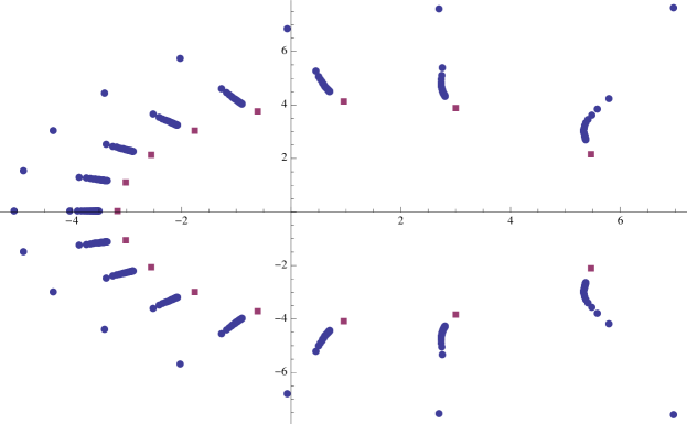
Figure 3. Exceptional zeros of the polynomials $L_{m,m+j}^{{\rm{II}}({\alpha})}(z)$ for $m=15$, ${\alpha}=14.01$ and $1\leq j\leq 22$. The squares denote the zeros of $L_{m}^{{(-{\alpha}-1)}}(z)$ to which the zeros of $L_{m,m+j}^{{\rm{II}}({\alpha})}(z)$ converge for $j\to\infty$.

5. Exceptional Jacobi polynomials

5.1. Definitions and identities

Let $m\geq 0$ be a fixed integer, and $\alpha,\beta$ real numbers. Let

(57) $$T_{{\alpha},{\beta}}[y]=(1-z^{2})y^{\prime\prime}+(\beta-\alpha+(\alpha+\beta+2)z)y^{\prime},$$

denote the Jacobi differential operator. The classical Jacobi polynomial of degree $n$ can be defined as the polynomial solution $y=P_{n}^{(\alpha,\beta)}(z)$ of the second order linear differential equation

(58) $$T_{{\alpha},{\beta}}[y]=-n(1+{\alpha}+{\beta}+n)y,\quad y(1)=\frac{({\alpha}+1)_{n}}{n}.$$

Next, define

(59) $$T_{\alpha,\beta,m}[y] =T_{\alpha,\beta}[y]+(\alpha-\beta-m+1)my$$

$$\qquad-(\log P_{m}^{(-{\alpha}-1,{\beta}-1)})^{\prime}\,\Big{(}\beta(1-z)y+(1-z^{2})y^{\prime}\Big{)},$$

(60) $$A_{\alpha,\beta,m}[y] =(1-z)P_{m}^{(-{\alpha},{\beta})}\,y^{\prime}+(m-\alpha)P_{m}^{(-{\alpha}-1,{\beta}-1)}\,y,$$

(61) $$B_{\alpha,\beta,m}[y] =\frac{(1+z)y^{\prime}+(1+\beta)y}{P_{m}^{(-{\alpha},{\beta})}}.$$

The following operator factorizations can be verified by the application of elementary identities.

(62) $$T_{\alpha,\beta,m} =A_{\alpha+1,\beta-1,m}B_{\alpha+1,\beta-1,m}-(m-\alpha-1)(m+\beta),$$

(63) $$T_{\alpha,\beta} =B_{\alpha,\beta,m}A_{\alpha,\beta,m}-(m-\alpha)(m+\beta+1).$$

For $n\geq m$, we define the degree $n$ exceptional Jacobi polynomial to be

(64) $${\hat{P}}_{m,n}^{(\alpha,\beta)} =\frac{(-1)^{m+1}}{\alpha+1+j}\,A_{\alpha+1,\beta-1,m}\left[P_{j}^{(\alpha+1,\beta-1)}\right],\qquad j=n-m\geq 0,$$

(65) $$=\frac{(-1)^{m}}{\alpha+1+j}\left(\frac{1}{2}(1+{\alpha}+{\beta}+j)(z-1)P_{m}^{(-{\alpha}-1,{\beta}-1)}P_{j-1}^{(\alpha+2,\beta)}\right.$$

$$\qquad\qquad\qquad\left.+(\alpha+1-m)\,P_{m}^{(-{\alpha}-2,{\beta})}P_{j}^{(\alpha+1,\beta-1)}\right).$$

The exceptional polynomials and operator extend their classical counterparts

(66) $$T_{\alpha,\beta,0}[y] =T_{\alpha,\beta}[y],$$

(67) $${\hat{P}}_{0,n}^{(\alpha,\beta)} =P_{n}^{(\alpha,\beta)}.$$

By construction, these polynomials satisfy several identities, which we enumerate below. The factorizations (62) (63) give the intertwining relations

(68) $$A_{\alpha+1,\beta-1,m}T_{\alpha+1,\beta-1}=T_{\alpha,\beta,m}A_{\alpha+1,\beta-1,m},$$

(69) $$T_{\alpha+1,\beta-1}B_{\alpha+1,\beta-1,m}=B_{\alpha+1,\beta-1,m}T_{\alpha,\beta,m}.$$

From the above relations we can derive the eigenvalue equation for the $X_{m}$-Jacobi polynomials

(70) $$T_{\alpha,\beta,m}\left[{\hat{P}}_{m,n}^{(\alpha,\beta)}\right]=-(n-m)(1+\alpha+\beta+n-m){{\hat{P}}^{(\alpha,\beta)}_{m,n}},\quad n\geq m.\\$$

The factorization (63) implies the following identity

(71) $$(-1)^{m}(\alpha+1+j)(\beta{{\hat{P}}^{(\alpha,\beta)}_{m,m+j}}+(z+1){{\hat{P}}_{m,m+j}^{(\alpha,\beta)^{\prime}}})=$$

$$\qquad\qquad(\alpha+1-m+j)(\beta+m+j){P^{(-\alpha-1,\beta-1)}_{m}}{P^{(\alpha+1,\beta-1)}_{j}}\,.$$

It will be useful to express ${\hat{P}}$ in a way that is symmetric in the dimension $j$ and the codimension $m$. Namely,

$$(-1)^{m}(\alpha+j){{\hat{P}}^{(\alpha-1,\beta+1)}_{m,m+j}}$$

(72) $$\qquad=(\alpha-m)P_{m}^{(-\alpha-1,\beta+1)}P_{j}^{(\alpha,\beta)}+(z-1)P_{m}^{(-\alpha,\beta)}{P_{j}^{(\alpha,\beta)}}^{\prime}$$

(73) $$\qquad=(\alpha+j){P^{(\alpha-1,\beta+1)}_{j}}{P^{(-\alpha,\beta)}_{m}}-(z-1)P_{j}^{(\alpha,\beta)}{P_{m}^{(-\alpha,\beta)}}^{\prime}\,.$$

The first equation is just a restatement of the definition (64), while the second identity follows from the classical relation

(74) $$(z-1){P_{j}^{(\alpha,\beta)}}^{\prime} =\alpha{P^{(\alpha,\beta)}_{j}}-(\alpha+j){P^{(\alpha-1,\beta+1)}_{j}}\,.$$

At the endpoints of the interval of orthogonality we have the following classical identities

(75) $${P^{({\alpha},{\beta})}_{n}}(-1) =(-1)^{n}\frac{({\beta}+1)_{n}}{n!},$$

(76) $${P^{({\alpha},{\beta})}_{n}}(1) =\frac{({\alpha}+1)_{n}}{n!},$$

which in the case of exceptional Jacobi polynomials yield the following generalizations

(77) $${{\hat{P}}^{(\alpha,\beta)}_{m,n}}(1) =\binom{\alpha+n-m}{n}\binom{n}{m},\quad n\geq m,$$

(78) $$=\frac{(\alpha+1-m)_{m+j}}{m!\,j!},\quad j=n-m,$$

(79) $${{\hat{P}}^{(\alpha,\beta)}_{m,m+j}}(-1) =(-1)^{j}\frac{(\beta+j+m)(1+\alpha-m+j)}{(1+\alpha+j)}\frac{(\beta+1)_{m-1}(\beta)_{j}}{m!\,j!}.$$

Define the 1st-order operators

(80) $${\hat{A}}_{\alpha,\beta,m}[y]=\frac{P_{m}^{(-{\alpha}-2,{\beta})}}{P_{m}^{(-{\alpha}-1,{\beta}-1)}}\left(y^{\prime}-(\log P_{m}^{(-{\alpha}-2,{\beta})})^{\prime}\,y\right)\,,$$

(81) $${\hat{B}}_{\alpha,\beta,m}[y]=(1-z^{2})\frac{P_{m}^{(-{\alpha}-1,{\beta}-1)}}{P_{m}^{(-{\alpha}-2,{\beta})}}\left[y^{\prime}-\left((\log P_{m}^{(-{\alpha}-1,{\beta}-1)})^{\prime}+\frac{\alpha+1}{1-z}-\frac{\beta+1}{1+z}\right)y\right]\,.$$

The following “shape-invariant” factorizations relate exceptional operators of the same codimension at different values of the parameters $\alpha,\beta$

(82) $${\hat{B}}_{\alpha,\beta,m}{\hat{A}}_{\alpha,\beta,m} =T_{\alpha,\beta,m}$$

(83) $${\hat{A}}_{\alpha,\beta,m}{\hat{B}}_{\alpha,\beta,m} =T_{\alpha+1,\beta+1,m}+2+\alpha+\beta.$$

The corresponding intertwining relations, namely,

(84) $$T_{\alpha+1,\beta+1,m}{\hat{A}}_{\alpha,\beta,m} ={\hat{A}}_{\alpha,\beta,m}T_{\alpha,\beta,m},$$

(85) $${\hat{B}}_{\alpha,\beta,m}T_{\alpha+1,\beta+1,m} =T_{\alpha,\beta,m}{\hat{B}}_{\alpha,\beta,m},$$

give rise to the lowering and raising relations for the exceptional Jacobi polynomials

(86) $$\left(\frac{{\hat{P}}_{m,n}^{(\alpha,\beta)}}{P_{m}^{(-{\alpha}-2,{\beta})}}\right)^{\prime}=\frac{1}{2}(n-m+\alpha+\beta+1)\left(\frac{P_{m}^{(-{\alpha}-1,{\beta}-1)}}{P_{m}^{(-{\alpha}-2,{\beta})}}\right)^{2}\,\frac{{\hat{P}}_{m,n-1}^{(\alpha+1,\beta+1)}}{P_{m}^{(-{\alpha}-1,{\beta}-1)}},\quad n\geq m+1,$$

(87) $$(1-z)^{-\alpha}(1+z)^{-\beta}\left((1-z)^{\alpha+1}(1+z)^{\beta+1}\frac{{\hat{P}}_{m,n}^{(\alpha+1,\beta+1)}}{P_{m}^{(-{\alpha}-1,{\beta}-1)}}\right)^{\prime}=$$

$$\qquad\qquad-2(n-m+1)\left(\frac{P_{m}^{(-{\alpha}-2,{\beta})}}{P_{m}^{(-{\alpha}-1,{\beta}-1)}}\right)^{2}\frac{{\hat{P}}_{m,n+1}^{(\alpha,\beta)}}{P_{m}^{(-{\alpha}-2,{\beta})}},\quad n\geq m.$$

As usual, we denote by $f^{\prime}(z)$ the derivative of $f$ with respect to the $z$ variable.

5.2. Orthogonality

The exceptional Jacobi polynomials are formally orthogonal with respect to ${\hat{W}}_{\alpha,\beta,m}(z)dz,\;-1\leq z\leq 1$, where

(88) $${\hat{W}}_{\alpha,\beta,m}(z)=\frac{(1-z)^{\alpha}(1+z)^{\beta}}{\left[P_{m}^{(-{\alpha}-1,{\beta}-1)}(z)\right]^{2}}.$$

In order to have orthogonality in the $L^{2}$ sense, additional conditions need to be imposed on the parameters $\alpha,\beta$, and $m$. The condition $\alpha,\beta>-1$ is necessary for the measure (88) to have finite moments of all orders. Another requirement is that the denominator $P_{m}^{(-{\alpha}-1,{\beta}-1)}$ does not vanish for $z\in(-1,1)$, which imposes extra conditions on $\alpha,\beta$, and $m$.

An analysis of the zeros of classical Jacobi polynomials can be found in Szegő’s book [43, Chapter 6.72]. First, let us recall that ${P^{(\alpha,\beta)}_{n}}(z)$ has a zero of multiplicity $k$ at $z=1$ if $\alpha=-k,\;k=1,\ldots,m$, and a zero of multiplicity $j$ at $z=-1$ if $\beta=-j,\;j=1,\ldots,m$.

We also mention the degenerate cases where

$$\deg{P^{(\alpha,\beta)}_{n}}=k\quad\text{ when }\quad n+\alpha+\beta+1=-k,\qquad k=0,1,\ldots,n-1.$$

For such parameter values the $n$th Jacobi polynomial has degree $<n$. In these degenerate cases (where ${\alpha}+{\beta}$ is a negative integer), we have

(89) $$\binom{{\alpha}+m}{m}{P^{({\alpha},{\beta})}_{n}}(z)=\binom{{\alpha}+n}{n}{P^{({\alpha},{\beta})}_{m}}(z),\quad{\alpha}+{\beta}=-1-m-n.$$

Since $\beta>-1$, the denominator has a zero at $z=-1$ if and only if $\beta=0$. However, the latter condition gives a weight with an overall factor of $(1+z)^{-1}$, which would violate the assumption that it has finite moments of all orders. Therefore we must impose $\beta\neq 0$. The condition that ${P^{(-\alpha-1,\beta-1)}_{m}}(z)\neq 0$ for $z\in(-1,1)$ is satisfied in exactly two cases

• Both $\beta$ and $\alpha+1-m$ $\in(-1,0)$.

• Both $\beta$ and $\alpha+1-m$ $\in(0,\infty)$.

For (A) we have $m-2<\alpha<m-1$, while for (B) we have $\alpha>m-1$. Therefore, in both cases ${P^{(-1-\alpha,\beta-1)}_{m}}(1)\neq 0$. According to identity (89), we also require

(90) $$\alpha+1-m-\beta\notin\{0,1,\ldots,m-1\}.$$

If this condition is violated, then $\deg{P^{(-\alpha-1,\beta-1)}_{m}}(z)<m$ and, therefore, the codimension (see below for discussion) is $\alpha+1-m-\beta$, rather than $m$. We therefore append condition (90) to the assumptions in (A) and (B), to complete the following

Proposition 5.1.

Suppose that $m\geq 1$. The measure ${\hat{W}}_{\alpha,\beta,m}dz,\;z\in(-1,1)$ is positive definite with finite moments of all orders if and only if $\alpha,\beta,m$ satisfy one of the following conditions

• $\beta,\alpha+1-m\in(-1,0)$.

• $\beta,\alpha+1-m\in(0,\infty)$.

In order to ensure that $\deg P_{m}^{(-\alpha-1,\beta-1)}=m$ it is also necessary to require that $\alpha+1-m-\beta\notin\{0,1,\ldots,m-1\}$.

5.3. Exceptional Flag

Let us define the following codimension $m$ polynomial flag $\{U_{\alpha,\beta,m,j}\}_{j=1}^{\infty}$ where

$$U_{\alpha,\beta,m,j}=\{f(z)\in\mathcal{P}_{m+j-1}(z):P_{m}^{(-{\alpha}-1,{\beta}-1)}|(1+z)f^{\prime}+\beta f\}.$$

At the level of flags, the factorizations (62) (63) correspond to the linear isomorphisms

$$A_{\alpha+1,\beta-1,m}:\mathcal{P}_{j-1}\to U_{\alpha,\beta,m,j},\quad B_{\alpha+1,\beta-1,m}:U_{\alpha,\beta,m,j}\to\mathcal{P}_{j-1},\quad j=1,2,\ldots.$$

Thus, the exceptional polynomials ${{\hat{P}}^{(\alpha,\beta)}_{m,m+j}}$ give a basis of the flag $\{U_{\alpha,\beta,m,j}\}_{j=1}^{\infty}$

Proposition 5.2.

Suppose that $\alpha,\beta,m$ satisfy either condition (A) or condition (B). Then ${\hat{P}}_{m,m+j}^{(\alpha,\beta)}(z)$ is the unique polynomial in $U_{\alpha,\beta,m,j}$, orthogonal to $U_{\alpha,\beta,m,j-1}$ with respect to ${\hat{W}}_{\alpha,\beta,m}\,dz,\;z\in(-1,1)$ that satisfies the normalizing condition (77).

Once we have analyzed the underlying factorizations that give rise to $X_{m}$-Jacobi polynomials, and the conditions on the parameters that ensure their $L^{2}$-orthogonality, we can now turn our attention to describing some properties of their zeros.

5.4. Zeros of exceptional Jacobi polynomials

Let us refer to the real zeros of ${{\hat{P}}^{(\alpha,\beta)}_{m,m+j}}(z)$ in $z\in(-1,1)$ as the regular zeros. All other zeros, whether in $(-\infty,-1)\cup(1,\infty)$, or complex, will be said to be exceptional zeros.

Proposition 5.3.

Suppose that $\alpha,\beta,m$ obey either condition (A) or condition (B). Then the regular zeros of ${{\hat{P}}^{(\alpha,\beta)}_{m,m+j}}(z)$ are simple.

Proof.

This follows from (64) (71) and the simplicity of the zeros of classical Jacobi polynomials. ∎

Proposition 5.4.

Suppose that $\alpha,\beta,m$ obey either condition (A) or condition (B). Then ${{\hat{P}}^{(\alpha,\beta)}_{m,m+j}}$ has exactly $j$ regular zeros and $m$ exceptional zeros.

Proof.

We begin by showing that ${\hat{P}}_{m,m+j}^{(\alpha,\beta)}$ has at least $j$ regular zeros by induction on $j$. The case $j=0$ is trivial. Suppose now that the proposition has been established for $j\geq 0$. Note that $\alpha+1,\beta+1,m$ always belong to class B by hypothesis. We observe also [43, Chapter 6.72] that $P_{m}^{(-{\alpha}-1,{\beta}-1)}(z)$ and $P_{m}^{(-{\alpha}-2,{\beta})}(z)$ have no zeros in $z\in[-1,1]$. Let $\zeta_{1},\ldots,\zeta_{i},\;i\geq j$, be the regular zeros of ${\hat{P}}_{m,m+j}^{(\alpha+1,\beta+1)}$. By (87) and Rolle’s theorem, ${\hat{P}}_{m,m+j+1}^{(\alpha,\beta)}(z)$ has at least one zero in each of the intervals $(\zeta_{1},\zeta_{2}),(\zeta_{2},\zeta_{3}),\ldots,(\zeta_{i-1},\zeta_{i})$. There will also be a zero in $(-1,\zeta_{1})$ and a zero in $(\zeta_{i},1)$, for a total of at least $i+1$ zeros.

We conclude by showing that ${\hat{P}}_{m,m+j}^{(\alpha,\beta)}$ has at most $j$ regular zeros. The proof is again by induction on $j$. Observe that

$${\hat{P}}_{m,m}^{(\alpha,\beta)}=(-1)^{m}\left(\frac{\alpha+1-m}{\alpha+1+j}\right)P_{m}^{(-{\alpha}-2,{\beta})},$$

and the latter has no zeros in $[-1,1]$. Relation (86) shows that between two regular zeros of ${\hat{P}}_{m,m+j}^{(\alpha,\beta)}$ there is at least one zero of ${\hat{P}}_{m,m+j-1}^{(\alpha+1,\beta+1)}$. Hence, if we assume that the latter has at most $j-1$ regular zeros, then the former has at most $j$ regular zeros. ∎

5.5. Asymptotic behaviour of the zeros

Our next goal is to derive a representation for the $X_{m}$-Jacobi polynomials that is amenable to asymptotic analysis.

Proposition 5.5.

The following identity holds:

(91) $$(-1)^{m}{\hat{P}}_{m,m+j}^{(\alpha,\beta)}=$$

$$\qquad\frac{\alpha-\beta-m+1}{1+\alpha+j}{P^{(-\alpha,\beta)}_{m-1}}\left(\frac{j}{\alpha+\beta+2j}{P^{(\alpha,\beta)}_{j}}-\frac{\alpha+j}{\alpha+\beta+2j}{P^{(\alpha,\beta)}_{j-1}}\right)+$$

$$\qquad\left(\frac{1+\alpha-m}{1+\alpha+j}{P^{(-2-\alpha,\beta)}_{m}}+\frac{j}{1+\alpha+j}{P^{(-\alpha-1,\beta-1)}_{m}}\right){P^{(\alpha,\beta)}_{j}}\,.$$

Proof.

We begin with (73) and apply (74) as well as the following classical identities:

$${P^{(1+\alpha,\beta-1)}_{j}} ={P^{(\alpha+1,\beta)}_{j-1}}+{P^{(\alpha,\beta)}_{j}}$$

$$(\alpha+\beta+2j)(z-1){P^{(\alpha+1,\beta)}_{j-1}} =2j{P^{(\alpha,\beta)}_{j}}-2(\alpha+j){P^{(\alpha,\beta)}_{j-1}}$$

∎

Proposition 5.6.

Suppose that $\alpha,\beta>-1$. As $j\to\infty$ we have the following asymptotic behaviour for $z$ in compact sets of $\mathbb{C}\backslash[-1,1]$

(92) $${{\hat{P}}^{(\alpha,\beta)}_{m,m+j}}-(-1)^{m}P_{m}^{(-{\alpha}-1,{\beta}-1)}P_{j}^{({\alpha},{\beta})}\rightrightarrows 0,\qquad j\to\infty.$$

Proof.

We make use of the following well known ratio asymptotics formula for classical Jacobi polynomials:

(93) $$\frac{{P^{(\alpha,\beta)}_{j-1}}(z)}{{P^{(\alpha,\beta)}_{j}}(z)}\rightrightarrows\frac{1}{z+\sqrt{z^{2}-1}},\quad z\notin[-1,1].$$

The conclusion now follows directly from (91). ∎

As a straightforward consequence, the following corollary describes the asymptotic behaviour of the zeros of exceptional Jacobi polynomials.

Corollary 5.1.

The $j$ regular zeros of ${{\hat{P}}^{(\alpha,\beta)}_{m,m+j}}$ approach the zeros of the classical Jacobi polynomial ${P^{(\alpha,\beta)}_{j}}$ as $j\to\infty$, while the $m$ exceptional zeros of ${{\hat{P}}^{(\alpha,\beta)}_{m,m+j}}$ approach the zeros of ${P^{(-\alpha-1,\beta-1)}_{m}}$.

The Heine-Mehler formula for the classical Jacobi polynomials states

(94) $$n^{-\alpha}{P^{(\alpha,\beta)}_{n}}(\cos(z/n))\rightrightarrows(z/2)^{-\alpha}J_{\alpha}(z).$$

The $X_{m}$-Jacobi polynomials satisfy a generalized Heine-Mehler formula, given by the following proposition.

Proposition 5.7.

When $n\to\infty$, we get

(95) $$n^{-\alpha}{{\hat{P}}^{(\alpha,\beta)}_{m,n}}(\cos(z/n))\rightrightarrows(-1)^{m}(z/2)^{-\alpha}\binom{m-1-\alpha}{m}J_{\alpha}(z),\quad n\geq m.$$

Proof.

Taking the limit $j\to\infty$ in (91) and using the classical Heine-Mehler formula (94) leads to the desired result, keeping in mind also that

$${P^{(-\alpha-1,\beta-1)}_{m}}(1)=\binom{m-1-\alpha}{m}.$$

∎

6. Summary and Open problems

We have provided suitable representations of exceptional polynomials in terms of their classical counterparts by exploiting the isospectral Darboux transformations that connect them. These representations allow to derive Heine-Mehler type formulas for the exceptional Jacobi and Laguerre polynomials, which describe the asymptotic behaviour of their regular zeros (those lying in the interval of orthogonality). The behaviour of the regular zeros of exceptional polynomials follows the same Bessel asymptotics as the zeros of their classical counterparts. We have also proved interlacing between the zeros of exceptional and classical polynomials, while the zeros of consecutive exceptional polynomials also interlace according to their Sturm-Liouville character. As for the exceptional zeros (those lying outside the interval of orthogonality) we have established their number and location and we have proved that for fixed codimension $m$ and large degree $n$ they approach the zeros of a classical polynomial. We have performed a careful analysis of the admissible ranges of the parameters that ensure a well defined Sturm-Liouville problem. We have also given raising and lowering relations for the exceptional polynomials. These relations correspond to a shape-invariant factorization, i.e. a Darboux transformation that falls within the same class of operators, with a shift in the parameters (see for instance (43)–(46)), and they imply that the associated potentials in quantum mechanics will be exactly solvable and shape invariant.

It was recently noticed that more families of exceptional orthogonal polynomials can be constructed through multi-step Darboux or Darboux-Crum transformations [18], an idea that has been further developed in [23, 35, 39]. In this work we have analyzed the zeros of exceptional orthogonal polynomials that can be obtained from the classical ones by a 1-step Darboux transformation. These polynomials can be written as a first order linear differential operator acting on their classical counterparts and the exceptional weight is a classical weight divided by the square of a classical polynomial with zeros outside the interval of orthogonality. An open problem is to extend this analysis to multi-step exceptional families, where exceptional polynomials are obtained by the action of an $m$-th order differential operator.

We believe that all exceptional orthogonal polynomials can be obtained from a classical system by a multi-step Darboux transformation, [20], and the exceptional weight for these systems will have in its denominator the Wronskian of all the factorizing functions, which are essentially classical orthogonal polynomials. The characterization of all such Wronskians whose zeros lie outside the interval of orthogonality becomes then a crucial question.

It is trivial to know the location of the zeros of a classical polynomial, and therefore to constrain its parameters so that they fall outside the interval of orthogonality for the exceptional weight to be regular. The question becomes much more involved when dealing with a Wronskian of classical polynomials as it happens in the multi-step case. However, this question must be addressed in order to select those multistep weights that are non-singular.

The position of the zeros for Wronskians of consecutive Hermite polynomials have been investigated numerically by Clarkson [4] since these functions appear as rational solutions to nonlinear differential equations of Painlevé type, [5]. A further numerical analysis together with some conjectures in a more general case have been recently put forward by Felder et al.[10], in connection with the theory of monodromy free potentials. We stress that a Wronskian of classical polynomials might have no real zeros even if the polynomials themselves do. The Adler-Krein theorem [1, 30] provides a useful criterion to identify these cases, and it is actually a much more general result for eigenfunctions of a Schrödinger operator, not just polynomials. A generalization of this result is being carried out by Grandati, who is extending the analysis to factorizing functions of isospectral Darboux transformations [23], as opposed to the Adler-Krein case which refers only to state-deleting Darboux transformations, for which the factorizing functions are true $L^{2}$ eigenfunctions. The most general problem of Wronskians that involve factorizing functions of mixed type remains unsolved.

Acknowledgements

The research of the first author (DGU) has been supported by Dirección General de Investigación, Ministerio de Ciencia e Innovación of Spain, under grant MTM2009-06973. The work of the second author (FM) has been supported by Dirección General de Investigación, Ministerio de Ciencia e Innovación of Spain, grant MTM2009-12740-C03-01. The research of the thirds author (RM) was supported in part by NSERC grant RGPIN-228057-2009.

References

- [1] V. E. Adler, A modification of Crum’s method, Theor. Math. Phys. 101 (1994) 1381–1386.
- [2] S. Bochner, Über Sturm-Liouvillesche Polynomsysteme, Math. Z. 29 (1929), 730-736.
- [3] M. I Bueno, F. Marcellán, Darboux Transformation and Perturbation of Linear Functionals, Linear Algebra Appl. 384 (2004) 215–242.
- [4] P.A. Clarkson, The fourth Painlevé equation and associated special polynomials. J. Math. Phys. 44 (2003), 5350–5374.
- [5] P.A. Clarkson, On rational solutions of the fourth Painlevé equation and its Hamiltonian, CRM Proc. Lect. Notes 39 (2005) 103–118.
- [6] M. M. Crum, Associated Sturm-Liouville systems, Quart. J. Math. 6 (1955) 121.
- [7] G. Darboux Théorie Générale des Surfaces vol 2, Gauthier-Villars, Paris, 1888.
- [8] D. Dutta and P. Roy, Conditionally exactly solvable potentials and exceptional orthogonal polynomials, J. Math. Phys. 51 (2010) 042101.
- [9] D. Dutta and P. Roy, Darboux transformation, exceptional orthogonal polynomials and information theoretic measures of uncertainty, in Algebraic aspects of Darboux transformations, quantum integrable systems and supersymmetric quantum mechanics. P. Acosta-Humánez et al. Eds. Contemp. Math. 563 (2012) 33–50.
- [10] G. Felder, A.D. Hemery, and A.P. Veselov, Zeroes of Wronskians of Hermite polynomials and Young diagrams, (2012) arXiv:1005.2695
- [11] D. Gómez-Ullate, N. Kamran and R. Milson, The Darboux transformation and algebraic deformations of shape-invariant potentials, J. Phys. A 37 (2004) 1789–1804.
- [12] D. Gómez-Ullate, N. Kamran and R. Milson, Supersymmetry and algebraic Darboux transformations, J. Phys. A 37 (2004) 10065–10078.
- [13] D. Gómez-Ullate, N. Kamran and R. Milson, Quasi-exact solvability and the direct approach to invariant subspaces. J. Phys. A 38 (2005) 2005–2019.
- [14] D. Gómez-Ullate, N. Kamran and R. Milson, Quasi-exact solvability in a general polynomial setting, Inverse Problems, 23 (2007) 1915.
- [15] D. Gómez-Ullate, N. Kamran, and R. Milson, An extended class of orthogonal polynomials defined by a Sturm-Liouville problem, J. Math. Anal. Appl. 359 (2009) 352–367.
- [16] D. Gómez-Ullate, N. Kamran, and R. Milson, An extension of Bochner’s problem: exceptional invariant subspaces, J. Approx. Theory 162 (2010) 897–1006.
- [17] D. Gómez-Ullate, N. Kamran, and R. Milson, Exceptional orthogonal polynomials and the Darboux transformation, J. Phys. A 43 (2010) 434016.
- [18] D. Gómez-Ullate, N. Kamran, and R. Milson, Two-step Darboux transformations and exceptional Laguerre polynomials, J. Math. Anal. Appl., 387 (2012), 410–418.
- [19] D. Gómez-Ullate, N. Kamran, and R. Milson, On orthogonal polynomials spanning a non-standard flag, in Algebraic aspects of Darboux transformations, quantum integrable systems and supersymmetric quantum mechanics. P. Acosta-Humánez et al. Eds. Contemp. Math. 563 (2012) 51–72.
- [20] D. Gómez-Ullate, N. Kamran, and R. Milson, A conjecture on exceptional orthogonal polynomials, arXiv:1203.6857
- [21] Y. Grandati, Solvable rational extensions of the isotonic oscillator , Ann. Phys. 326 (2011) 2074–2090.
- [22] Y. Grandati, Solvable rational extensions of the Morse and Kepler-Coulomb potentials , J. Math. Phys. 52 (2011) 103505.
- [23] Y. Grandati, Multistep DBT and regular rational extensions of the isotonic oscillator, (2012) arXiv:1108.4503
- [24] C-L. Ho, Dirac(-Pauli), Fokker–Planck equations and exceptional Laguerre polynomials, Ann. Phys. 326 (2011) 797–807.
- [25] C-L. Ho and R. Sasaki, Zeros of the exceptional Laguerre and Jacobi polynomials, arXiv:1102.5669
- [26] R. Koekoek, P. A. Lesky, R. F. Swarttouw, Hypergeometric Orthogonal Polynomials and Their q-Analogues, Springer Monographs in Mathematics, Springer Verlag, Berlin 2010.
- [27] H. L. Krall, On orthogonal polynomials satisfying a certain fourth order differential equation, the Pennsylvania State College Studies, 6, State College PA, 1940.
- [28] A. M. Krall, Orthogonal polynomials satisfying fourth order differential equations, Proc. Roy. Soc. Edinburgh Sec. A 87 (1981), 271–288.
- [29] A. M. Krall, Hilbert Space, Boundary Value Problems, and Orthogonal Polynomials, in Operator Theory, Advances and Applications. Vol 133. Birkhauser, Basel. 2002.
- [30] M.G. Krein, On a continual analogue of a Christoffel formula from the theory of orthogonal polynomials (Russian), Dokl. Akad. Nauk SSSR (N.S.), 113 (1957) 970-973.
- [31] P. Lesky, Die Charakterisierung der klassischen orthogonalen Polynome durch SturmLiouvillesche Differentialgleichungen, Arch. Rat. Mech. Anal. 10 (1962), 341–352.
- [32] B. Midya and B. Roy, Exceptional orthogonal polynomials and exactly solvable potentials in position dependent mass Schrödinger Hamiltonians, Phys. Lett. A 373(45) (2009) 4117–4122.
- [33] C. Quesne, Exceptional orthogonal polynomials, exactly solvable potentials and supersymmetry, J. Phys. A 41 (2008) 392001–392007.
- [34] C. Quesne, Solvable rational potentials and exceptional orthogonal polynomials in supersymmetric quantum mechanics, SIGMA 5 (2009) 084.
- [35] C. Quesne, Higher-order SUSY, exactly solvable potentials, and exceptional orthogonal polynomials, Mod. Phys. Lett. A 26 (2011) 1843-1852.
- [36] S. Odake and R. Sasaki, Infinitely many shape invariant potentials and new orthogonal polynomials, Phys. Lett. B 679 (2009) 414.
- [37] S. Odake and R. Sasaki, Another set of infinitely many exceptional () Laguerre polynomials, Phys. Lett. B684 (2010) 173–176.
- [38] S. Odake and R. Sasaki, Infinitely many shape invariant potentials and cubic identities of the Laguerre and Jacobi polynomials, J. Math. Phys. 51 (2010) 053513.
- [39] S. Odake and R. Sasaki, Exactly solvable quantum mechanics and infinite families of multi-indexed orthogonal polynomials, Phys. Lett. B 702 (2011), 164–170.
- [40] S. Odake and R. Sasaki, Discrete quantum mechanics, J. Phys. A 44 (2011), 353001.
- [41] E. Routh, On some properties of certain solutions of a differential equation of the second order, Proc. London Math. Soc. 16 (1884), 245–261.
- [42] R. Sasaki, S. Tsujimoto, and A. Zhedanov, Exceptional Laguerre and Jacobi polynomials and the corresponding potentials through Darboux-Crum transformations, J. Phys. A 43 (2010) 315204.
- [43] G. Szegő, Orthogonal polynomials, Amer. Math. Soc. Colloq. Publ. 23, American Mathematical Society, Providence, Rhode Island 1975. Fourth Edition.
- [44] T. Tanaka, -fold Supersymmetry and quasi-solvability associated with -Laguerre polynomials, J. Math. Phys. 51 (2010) 032101
- [45] A. Zhedanov. Rational spectral transformations and orthogonal polynomials, J. Comput. Appl. Math. 85 (1997), no. 1, 67–86.