Partial freeness of random matrices

Abstract.

We investigate the implications of free probability for finite-dimensional, Hermitian random matrices. While most pairs of matrices are not free, they can nevertheless be characterized by the joint moments which violate freeness. We use this to extend the notion of freeness to an intermediate property which we call partial freeness. Furthermore, we can calculate the deviation of the true density of states from the free convolution using asymptotic moment expansions, whose coefficients have a natural combinatorial interpretation over weights of closed paths. We have developed computer programs for characterizing partial freeness from either numerical samples of matrices or analytic eigenvalue distributions. Our results provide a rich extension of free probability into the realm of finite linear algebra, with freeness emerging in limiting cases.

Introduction

Free probability has received much attention since its discovery as an algebraic structure for noncommuting operators.[25] Subsequently, it has found a place in combinatorics with the deep relationship between free cumulants and noncrossing partitions.[16, 17] Free probability for random matrices usually focuses on the asymptotic freeness of infinite matrices.[27, 2] In contrast, we investigate here how free probability offers us new perspectives on finite-dimensional matrices. We develop and extend the notion of freeness to finite random matrices using linear algebra and elementary statistics, without requiring intricate knowledge of operator algebras or combinatorics.

In this paper, we consider the problem of calculating eigenvalues of sums of finite matrices given the eigenvalues of the individual matrices, as an illustration of the power of free probability theory. In general, the eigenvalues of the sum of two matrices $A+B$ are not simply the sums of the eigenvalues of the individual matrices $A$ and $B$;[11] as matrices do not generally commute, the addition of eigenvalues must take into account the relative orientations of eigenvectors. However, free probability does allows us to do this calculation in the limiting case where the rotation matrix between the two bases is so random as to be uniformly oriented, i.e. of uniform Haar measure. The matrices $A$ and $B$ are then said to be in generic position, or free, and the eigenvalue spectrum of $A+B$ converges, in a sense, to the additive free convolution $A\boxplus B$ of two random matrices $A$ and $B$ as the matrix dimensions increase to infinity.[16]

A natural question to ask is how accurately $A\boxplus B$ approximates the exact eigenvalue spectrum, or density of states (d.o.s.), of the sum $A+B$ when the individual matrices are known to be noncommuting but not necessarily free. We seek to quantify this statement in this paper. In addition to classifying two random matrices as being free or not free relative to each other, we can characterize them as having an intermediate, graduated property which we call partial freeness, and furthermore we are able to quantify the leading-order discrepancy between freeness and partial freeness. This has already helped us explain the unexpected accuracy of approximations to the Hamiltonians of disordered condensed matter systems.[4]

We begin with a brief, self-contained review of free probability from a random matrix theoretic perspective, and provide an elementary illustration of how computing the additive free convolution using an integral transform allows us to calculate the d.o.s. for the sum of free random matrices. Next, we recap how the additive free convolution can also be approached via the moments of random matrices, and in particular how both classical and free independence can be interpreted as imposing precise rules for the decomposition of joint moments of arbitrary orders. We then show how we can generalize this to the notion of partial freeness and describe a procedure for detecting it numerically from samples of random matrices.

1. Freeness of two matrices

We use the notation $\left\langle\cdot\right\rangle$ for the normalized expected trace (n.e.t.) $\frac{1}{N}\mathbb{E}\mbox{ Tr}\cdot$ of a $N\times N$ matrix.

Definition 1.

The random matrices $A$ and $B$ are free (or synonymously, freely independent) with respect to the n.e.t. if for all $k\in\mathbb{N}$,

(1.1) $$\left\langle p_{1}\!\left(A\right)q_{1}\!\left(B\right)p_{2}\!\left(A\right)q_{2}\!\left(B\right)\cdots p_{k}\!\left(A\right)q_{k}\!\left(B\right)\right\rangle=0$$

for all polynomials $p_{1},q_{1},p_{2},q_{2},\dots p_{k},q_{k}$ such that $\left\langle p_{1}\!\left(A\right)\right\rangle=\left\langle q_{1}\!\left(B\right)\right\rangle=\cdots=0$.[25, Definition 4.2]

This generalizes the notion of (classical) independence of scalar random variables: were $A$ and $B$ to commute, the preceding with $k=1$ would suffice.

Fact 2.

The preceding is equivalent to defining free independence using the special case of the centering polynomials $p_{i}\left(x\right)=x^{n_{i}}-\left\langle x^{n_{i}}\right\rangle$, $q_{i}\left(x\right)=x^{m_{i}}-\left\langle x^{m_{i}}\right\rangle$, $i=1,\dots,k$ for positive integers $n_{1},m_{1},\dots,n_{k},m_{k}$.[25, Proposition 4.3]

That this is sufficient follows from the linearity of the n.e.t. In principle, this would allow us to check if two matrices $A$ and $B$ were free by checking that all centered joint moments

$$\left\langle\left(A^{n_{1}}\!-\!\left\langle A^{n_{1}}\right\rangle\right)\left(B^{m_{1}}\!-\!\left\langle B^{m_{1}}\right\rangle\right)\cdots\left(A^{n_{k}}\!-\!\left\langle A^{n_{k}}\right\rangle\right)\left(B^{m_{k}}\!-\!\left\langle B^{m_{k}}\right\rangle\right)\right\rangle$$

vanish for all positive exponents $n_{1}$,$m_{1}$,$\ldots$,$n_{k}$,$m_{k}$. However, this is numerically impractical due to the need to check joint moments of all orders, as well as the presence of fluctuations from sampling error if using Monte Carlo, which causes the higher order joint moments to converge slowly. In practice, it is far easier to check for freeness by examining how the d.o.s. of the exact sum $A+B$ converges to the p.d.f. defined by the free convolution $A\boxplus B$,[26] which we will now define.

1.1. The free convolution

Definition 3.

The $R$-transform of the p.d.f. $f_{A}$, denoted by $R_{A}$, is defined implicitly via the following Cauchy transform:[25, 16]

(1.2) $$w=\lim_{\epsilon\downarrow 0}\int_{\mathbb{R}}\frac{f_{A}\left(z\right)}{R_{A}\left(w\right)-\left(z+i\epsilon\right)}dz.$$

Some intuition for the $R$-transform may be achieved by expanding the Cauchy integral as a formal power series:

(1.3) $$G_{A}\left(w\right)=\lim_{\epsilon\downarrow 0}\int_{\mathbb{R}}\frac{f_{A}\left(z\right)}{w-z-i\epsilon}dz=\sum_{k=0}^{\infty}\frac{\mu_{k}\left(A\right)}{w^{k+1}},$$

where $\mu_{k}$ is the $k$th moment

(1.4) $$\mu_{k}\left(A\right)=\int_{\mathbb{R}}x^{k}f_{A}\left(x\right)dx=\left\langle A^{k}\right\rangle.$$

In other words, the Cauchy transform of a p.d.f. is a generating function of its moments. We then have that the $R$-transform $R_{A}$ inverts the Cauchy transform $G_{A}$ in the functional sense, i.e. that

(1.5) $$G_{A}\left(R_{A}\left(w\right)\right)=w.$$

Viewing both $G_{A}$ and $R_{A}$ as formal power series, the latter is simply the reversion of the former,[13, 8] in the sense that $R_{A}$ is a series in $w$ whose inverse with respect to composition is $G_{A}$ as a series in $1/z$. The coefficients of the $R$-transform are then the free cumulants $\nu_{k}$, i.e.

(1.6) $$R_{A}\left(w\right)=\sum_{k=0}^{\infty}\nu_{k}w^{k-1},$$

with $\nu_{0}=1$. The free cumulants are particular combinations of moments $\nu_{k}=\nu_{k}\left(\mu_{1},\dots,\mu_{k}\right)$ which shall be made more explicit later.

Definition 4.

The free convolution $A\boxplus B$ is defined via its $R$-transform

(1.7) $$R_{A\boxplus B}\left(w\right)=R_{A}\left(w\right)+R_{B}\left(w\right)-\frac{1}{w}.$$

The free cumulants linearize the free convolution in the sense that for all $k>0$,[16, 17]

(1.8) $$\nu_{k}\left(A\boxplus B\right)=\nu_{k}\left(A\right)+\nu_{k}\left(B\right),$$

and the subtraction of $1/w$ produces a properly normalized p.d.f. by conserving $\nu_{0}\left(A\boxplus B\right)=\mu_{0}\left(A\boxplus B\right)=1$.

In Section 1.3, we show an example of calculating $f_{A\boxplus B}$ analytically via the $R$-transform. In general, such analytic calculations are hindered by the functional inversions required in (1.2). This has inspired interesting work in calculating $A\boxplus B$ numerically, such as in the RMTool package.[19, 18] We discuss instead an alternate strategy starting directly from numerical samples of random matrices, which generalizes naturally to general pairs of matrices. In situations where only the numerical samples are known, it may be convenient instead to use the result of Fact 7 described in the next section.

1.2. Free convolution from random rotations

Definition 5.

A square matrix $Q$ is a unitary/orthogonal/symplectic random matrix of Haar measure if for any constant unitary/orthogonal/symplectic matrix $P$, the integral of any function over $dQ$ is identical to the integral over $d\left(PQ\right)$ or that over $d\left(QP\right)$.

Example 6.

Unitary matrices of dimension $N=1$ are simply scalar unit complex phases of the form $e^{i\theta}$. Haar measure over $e^{i\theta}$ can be written simply as $\mbox{d}\theta/2\pi$. This is manifestly rotation invariant, as multiplying $e^{i\theta}$ by any constant phase factor $e^{i\phi}$ simply changes the measure to $\mbox{d}(\theta+\phi)/2\pi=\mbox{d}\theta/2\pi$.

Uniform Haar measure generalizes the concept of uniformity to higher dimensions by preserving the notion of invariance with respect to arbitrary rotations. Consequently, the eigenvalues of $Q$ lie uniformly on the unit circle on the complex plane.[6] Explicit samples can be generated numerically by performing $QR$ decompositions on $N\times N$ matrices sampled from the Gaussian orthogonal (unitary) ensemble.[5]

Fact 7.

For a pair of Hermitian (real symmetric) random matrices $A$ and $B$, the d.o.s. of $A+QBQ^{\dagger}$, where $Q$ is a unitary (orthogonal) random matrix of Haar measure, coincides with the p.d.f. of $A\boxplus B$ in the limit of infinitely large matrices $N\rightarrow\infty$.

Consider the diagonalization of $A=Q_{A}\Lambda_{A}Q_{A}^{\dagger}$ and $B=Q_{B}\Lambda_{B}Q_{B}^{\dagger}$. The d.o.s. of $A+QBQ^{\dagger}$ is identical to that of $\Lambda_{A}+\left(Q_{A}^{\dagger}QQ_{B}\right)\Lambda_{B}\left(Q_{B}^{\dagger}Q^{\dagger}Q_{A}\right)$, since these matrices are related by the similarity transformation $Q_{A}^{\dagger}\left(\cdot\right)Q_{A}$. However, the Haar property of $Q$ means that the d.o.s. of this matrix is identical to that of $\Lambda_{A}+Q\Lambda_{B}Q^{\dagger}$. This gives us another interpretation of free convolution: it describes the statistics resulting from adding two random matrices when the basis of one matrix is randomly rotated or “spun around” relative to the other. The information about the relative orientations of the two bases is effectively ignored, retaining only the knowledge that they are not parallel so that $A$ and $B$ do not commute.

The freeness of random matrices usually discussed only in the limit of infinitely large matrices, where it is called asymptotic freeness.[27] For example, two matrices sampled from the Gaussian ensembles (orthogonal, unitary or symplectic) are free.[16] Nevertheless, finite-dimensional random matrices can exhibit freeness as well. We now provide some examples and illustrate the analytic calculation of the free convolution using the $R$-transform.

1.3. Examples of free finite-dimensional matrices

Example 8.

Consider the $2\times 2$ real symmetric random matrices

(1.9) $$A\left(t\right)=U\left(t\right)\sigma_{z}U\left(-t\right),\quad B\left(t\right)=U\left(-t\right)\sigma_{z}U\left(t\right),$$

where $\sigma_{z}$ is the Pauli matrix $\left(\begin{array}[]{cc}1&0\\ 0&-1\end{array}\right)$, $U\left(t\right)$ is the rotation matrix $\left(\begin{array}[]{cc}\cos t&\sin t\\ -\sin t&\cos t\end{array}\right)$, and the rotation angle $t$ is uniformly sampled on the interval $\left[0,\pi\right)$. By construction, the d.o.s. of $A\left(t\right)$ and $B\left(t\right)$ are identical; their eigenvalues have the p.d.f.

(1.10) $$f_{A}\left(x\right)=f_{B}\left(x\right)=\frac{1}{2}\left(\delta\left(x+1\right)+\delta\left(x-1\right)\right),$$

where $\delta\left(x\right)$ is the Dirac delta distribution. Furthermore, for any particular $t$, the sum of $A\left(t\right)$ and $B\left(t\right)$ can be written in the basis where $A\left(t\right)$ is diagonal as

(1.11) $$M\left(t\right)=\sigma_{z}+U\left(-2t\right)\sigma_{z}U\left(2t\right).$$

By construction, $U\left(2t\right)$ is of uniform Haar measure and so the d.o.s. of $M\left(t\right)$ is given exactly by the additive free convolution of $A\left(t\right)$ and $B\left(t\right)$.[27, 16] The $R$-transforms of $f_{A}$ and $f_{B}$ are

(1.12) $$R_{A}\left(w\right)=R_{B}\left(w\right)=\frac{1\pm\sqrt{1+4w^{2}}}{2w}.$$

Performing the free convolution,

(1.13) $$R_{A\boxplus B}\left(w\right)=R_{A}\left(w\right)+R_{B}\left(w\right)-\frac{1}{w}=\pm\frac{\sqrt{1+4w^{2}}}{w}.$$

Finally, we calculate the p.d.f. using the Plemelj inversion formula:

(1.14a) $$f_{A\boxplus B}\left(x\right) =\frac{1}{\pi}\left[\mbox{Im }R_{A\boxplus B}^{-1}\left(w\right)\right]_{w=x}$$

(1.14b) $$=\frac{1}{\pi\sqrt{4-x^{2}}},$$

which is the arcsine distribution on the interval $\left[-2,2\right]$, and we have retained only the positive root to obtain a nonnegative probability density. The odd moments all vanish by the even symmetry of $f_{\negthinspace A\boxplus B}$, and the even moments are the central binomial coefficients $\mu_{2n}\negthinspace\left(\negthinspace A\negthinspace\boxplus\negthinspace B\right)$ $=\binom{2n}{n}$.

This example shows that the free convolution of two discrete probability distributions can be a continuous probability distribution. In contrast, the classical convolution $A\star B$ produces the p.d.f.

(1.15) $$f_{A\star B}\left(x\right)=f_{A}\star f_{B}=\int_{\mathbb{R}}f_{A}\left(y\right)f_{B}\left(x-y\right)dy=\frac{1}{4}\left(\delta\left(x+2\right)+2\delta\left(x\right)+\delta\left(x-2\right)\right),$$

which is simply a discrete binomial distribution. The results of the two convolutions are plotted in Figure 1.

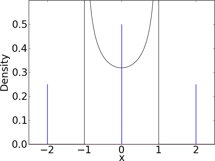
Figure 1. The d.o.s. $f_{A\boxplus B}\left(x\right)$ and $f_{A\star B}$$\left(x\right)$ for the free (dashed blue line) and classical convolutions (solid black bars) of the matrices in Example 1, as given in (1.14b) and (1.15) respectively. The heights of the lines in the plot of $f_{A\star B}$ indicate the point masses.

Here is another example of matrices with the same d.o.s. as before. This time, the matrices are not random at all.

Example 9.

The $2N\times 2N$ deterministic matrices

(1.16) $$A=\left(\begin{array}[]{ccccc}0&1\\ 1&0\\ &&0&1\\ &&1&0\\ &&&&\ddots\end{array}\right),\quad B=\left(\begin{array}[]{ccccc}0&&&&1\\ &0&1\\ &1&0\\ &&&\ddots\\ 1&&&&0\end{array}\right)$$

are asymptotically free as $N\rightarrow\infty$. Each consists of $N$ direct sums of the Pauli matrix $\sigma_{x}=\left(\begin{array}[]{cc}0&1\\ 1&0\end{array}\right)$, with $B$ having a basis shifted relative to $A$ with circulant (periodic) boundary conditions. The d.o.s. are the same as in the previous example and so the calculations of $A\boxplus B$ and $A\star B$ proceed identically. Considering the matrix $B^{\prime}$, being $B$ without the circulant entries on the lower left and upper right, we also have that $A$ and $B^{\prime}$ are asymptotically free as $N\rightarrow\infty$.

1.4. Comparison of free and classical convolutions

To conclude this introductory survey, we compare the free additive convolution $\boxplus$ and the classical convolution $\star$ in more detail. We note that the Fourier transform $\;\widehat{\cdot}\;$ turns classical convolutions into products according to the convolution theorem, i.e. $\widehat{f_{A}\star f_{B}}=\widehat{f_{A}}\widehat{f_{B}}$; taking the logarithm allows this to be written as a linear sum:

(1.17) $$\log\widehat{f_{A}\star f_{B}}=\log\widehat{f_{A}}+\log\widehat{f_{B}}.$$

Furthermore if $f_{A}$ and $f_{B}$ are p.d.f.s, then $\log\widehat{f_{A}}$ and $\log\widehat{f_{B}}$ can be identified as the corresponding (classical) cumulant generating functions, i.e. $\log\widehat{f_{A}}$ can be expanded in a formal power series

(1.18) $$\log\widehat{f_{A}}\left(w\right)=\sum_{k=0}^{\infty}\frac{\kappa_{n}\left(A\right)w^{n}}{n!},$$

where $\kappa_{n}\left(A\right)$ is the $n$th (classical) cumulant of $f_{A}$, and similarly for $f_{B}$. We have also have that $\kappa_{n}\left(A\star B\right)=\kappa_{n}\left(A\right)+\kappa_{n}\left(B\right)$ for $n\geq 1$, i.e. that cumulants linearize the convolution. Drawing an analogy between the cumulants $\kappa_{n}$ and the free cumulants $\nu_{n}$, the $R$-transform is often described as the free analogue of the log-Fourier transform, with the Cauchy transform being the analogue of the Fourier transform and the functional inversion playing the part analogous to the logarithm.

Finally, we note that the sum of two scalar random variables $a$ and $b$, sampled with p.d.f.s $f_{A}$ and $f_{B}$ respectively, itself has the resulting p.d.f. $f_{A\star B}$.[7] For matrices $A$ and $B$ with d.o.s. $f_{A}$ and $f_{B}$ respectively, then the matrix $A+\Pi B\Pi^{T}$, where $\Pi$ is a random permutation matrix, has d.o.s. $f_{A}\star f_{B}$. This is equivalent to the p.d.f. formed by picking an eigenvalue of $A$ at random and an eigenvalue of $B$ at random. In this sense, the discrete random permutation $\Pi$ which generates the classical convolution is the analogue of the continuous random rotation $Q$ of uniform Haar measure in free convolution.

Table 1 summarizes the analogies between the free and classical convolutions.

Table 1. Correspondence between the free and classical convolutions.

$A\boxplus B$	$A\star B$
$R$-transform $R$	log-Fourier transform $\log\hat{f}$
Cauchy transform $G$	Fourier transform $\hat{f}$
functional inversion	logarithm
free cumulants $\nu_{n}$	(classical) cumulants $\kappa_{n}$
Plemelj inversion	inverse Fourier transform
$A+QBQ^{\dagger}$	$A+\Pi B\Pi^{T}$
uniform Haar measure $Q$	random permutations $\Pi$

2. Density of states of sums of random matrices

The introductory examples show that if $A$ and $B$ are free, then the d.o.s. of $A+B$ can be calculated exactly without any detailed knowledge of the eigenvectors of $A$ and $B$. However, not all pairs of random matrices are free. Nevertheless, the free convolution can provide surprisingly accurate approximations to their d.o.s. even in the general case, and the degree of approximation can even be quantified by examining individual moments of the sum, $\mu_{n}\left(A+B\right)$ as shown in Section 15. In order to do this, however, we will first need to examine how each moment of $A+B$ subdivides into sums over joint moments of $A$ and $B$, and how the primordial definition of freeness in (1.1) determines what these moments must be for free $A$ and $B$. For simplicity, we assume in this paper that all necessary moments $\left\{\mu_{n}\right\}$ exist, so that the moments capture all the information contained in the corresponding p.d.f. For random matrices, this simply means that all powers of the matrix must have a finite n.e.t.

2.1. Calculating moments of $A+B$ from the joint moments of $A$ and $B$

For general $A$ and $B$, it is possible to characterize the d.o.s. of $A+B$ completely without constructing the sum and diagonalizing it if all their joint moments are known. We can then calculate all the moments $\left\{\mu_{n}\left(A+B\right)\right\}$ from the definition of the moment of a random matrix:

(2.1a) $$\mu_{n}= \left\langle\left(A+B\right)^{n}\right\rangle$$

(2.1b) $$= \langle A^{n}+A^{n-1}B+A^{n-2}BA+\cdots+BA^{n-1}+A^{n-2}B^{2}+\cdots+B^{2}A^{n-2}+\cdots+B^{n}\rangle$$

(2.1c) $$= \left\langle A^{n}\right\rangle+n\left\langle A^{n-1}B\right\rangle+n\left\langle A^{n-2}B^{2}\right\rangle+\cdots+\left\langle B^{n}\right\rangle.$$

The second equality follows directly from the noncommutative binomial expansion of (2.1b), and the third equality follows from the linearity of $\left\langle\cdot\right\rangle$ and its cyclic invariance, i.e. $\left\langle AB\right\rangle=\left\langle BA\right\rangle$.

We refer to (2.1c) as the word expansion of $\mu_{n}$. As written, there are $2^{n}$ terms in (2.1b) but some of them yield the same n.e.t. in (2.1c) identically because of cyclic invariance. The equivalence classes defined by grouping identical terms in this manner are exactly those of combinatorial necklaces.[12, 20]

Definition 10.

An $\left(n,k\right)$-word $W$ is a string of $n$ symbols, each of which can have any of $k$ values. An $\left(n,k\right)$-necklace $\left[\mathcal{N}\right]$ is the equivalence class over $\left(n,k\right)$-words $W$ with respect to cyclic permutations $\Pi$ of length $n$, i.e.

(2.2) $$\left[\mathcal{N}\right]=\left\{w\in W|\exists\pi\in\Pi:\;\mathcal{N}=\pi w\right\}.$$

There are efficient algorithms for enumerating all $\left(n,k\right)$-necklaces for a given $n$ and $k$.[21, 22] Furthermore, the total number of terms in the word expansion (2.1c) is well-known:

Fact 11.

The number of $\left(n,k\right)$-necklaces is

(2.3) $$N\left(n,k\right)=\frac{1}{n}\sum_{d|n}\phi\left(d\right)k^{n/d}=\frac{1}{n}\sum_{i=1}^{n}k^{\gcd\left(i,n\right)},$$

where $d|n$ means that $d$ divides $n$, $\phi$ is the Euler totient function, and $\gcd$ is the greatest common divisor.[12, 20] By definition, $\phi\left(d\right)$ is the number of integers $m$ in the range $1\leq m\leq d$ that are relatively prime to $d$, i.e. $gcd\left(d,m\right)=1$.

In addition, we can determine the multiplicity of each term in (2.1c), which is identical to the number of words in the equivalence class defined by each corresponding particular necklace. We state this very simple fact without proof and provide an example.

Fact 12.

Let $m=\#\left(\left[\mathcal{N}\right]\right)$ be the number of $\left(n,k\right)$-words belonging to the equivalence class that defines the necklace $\left[\mathcal{N}\right]$. Then $m$ is the length of the longest cyclic permutation that leaves any word $W\in\mathcal{N}$ unchanged, i.e. it is the length of the longest subword $S$ of a word $W\in\mathcal{N}$ such that $W=S^{n/m}$.

Example 13.

The necklace $\left[AABAAB\right]=\left[A^{2}BA^{2}B\right]$ is an equivalence class over $\left(6,2\right)$-words of size 3, since applying a (one-symbol) cyclic permutation three times leaves $A^{2}BA^{2}B$ unchanged:

(2.4) $$AABAAB\mapsto ABAABA\mapsto BAABAA\mapsto AABAAB,$$

i.e. $\#\left(\left[A^{2}BA^{2}B\right]\right)=3$ which follows from the fact that $AABAAB=\left(AAB\right)^{2}$.

The algorithmic enumeration of necklaces and their multiplicities allow us to sum the joint moments in the word expansion (2.1c) to obtain $\mu_{n}$. As $N\left(n,k\right)=\mathcal{O}\left(k^{n}/n\right)$ asymptotically as $n\rightarrow\infty$, the word expansion saves approximately a factor of $n$ in effort relative to working with the naive noncommutative binomial expansion, which has $k^{n}$ terms.

2.2. Decomposition rules for joint moments

We have reduced the problem of calculating $\mu_{n}$ to that of calculating joint moments; each has the form $\left\langle A^{n_{1}}B^{m_{1}}\cdots A^{n_{k}}B^{m_{k}}\right\rangle$ for positive integers $n_{1}$, $m_{1}$, $\ldots$, $n_{k}$, $m_{k}$. In general, this is not the most compact way to specify the relationship between $A$ and $B$. However, classical and free independence each provide a prescription for computing such joint moments in terms of the pure moments $\left\langle A\right\rangle$, $\left\langle A^{2}\right\rangle$, $\ldots$ and $\left\langle B\right\rangle$, $\left\langle B^{2}\right\rangle$, $\ldots$ of $A$ and $B$ respectively.

Fact 14.

For classically independent random matrices $A$ and $B$,

(2.5) $$\left\langle A^{n_{1}}B^{m_{1}}\cdots A^{n_{k}}B^{m_{k}}\right\rangle=\left\langle A^{n_{1}+\cdots+n_{k}}B^{m_{1}+\cdots+m_{k}}\right\rangle=\left\langle A^{n_{1}+\cdots+n_{k}}\right\rangle\left\langle B^{m_{1}+\cdots+m_{k}}\right\rangle,$$

i.e. $A$ and $B$ behave as if they commute.[16]

The analogous rule for free independence is more complicated; however, an implicit formula can be derived from the primordial definition of freeness in (1.1) by using the linearity of the n.e.t.:

(2.6a) $$0= \left\langle\left(A^{n_{1}}-\left\langle A^{n_{1}}\right\rangle\right)\left(B^{m_{1}}-\left\langle B^{m_{1}}\right\rangle\right)\left(A^{n_{k}}-\left\langle A^{n_{k}}\right\rangle\right)\left(B^{m_{k}}-\left\langle B^{m_{k}}\right\rangle\right)\right.$$

$$= \left\langle A^{n_{1}}B^{m_{1}}\cdots A^{n_{k}}B^{m_{k}}\right\rangle$$

$$-\left\langle A^{n_{1}}\right\rangle\left\langle A^{n_{2}}B^{m_{2}}\cdots A^{n_{k}}B^{m_{k}+m_{1}}\right\rangle-\left\langle B^{m_{1}}\right\rangle\left\langle A^{n_{1}+n_{2}}B^{m_{2}}\cdots A^{n_{k}}B^{m_{k}}\right\rangle$$

(2.6b) $$+\dots+\left(-1\right)^{\sum_{i=1}^{k}\left(n_{i}+m_{i}\right)}\left\langle A^{n_{1}}\right\rangle\cdots\left\langle A^{n_{k}}\right\rangle\left\langle B^{m_{1}}\right\rangle\cdots\left\langle B^{m_{k}}\right\rangle,$$

which can be rearranged immediately to give a recurrence relation for the joint moment $\left\langle A^{n_{1}}B^{m_{1}}\cdots A^{n_{k}}B^{m_{k}}\right\rangle$ in terms of joint moments of lower order.

3. Partial freeness

The main result of our paper is to show that the following notion of partial freeness is a useful generalization of freeness, particularly for finite random matrices.

Definition 15.

Two random matrices $A$ and $B$ are partially free to order $p$ if the first difference between $A+B$ and $A\boxplus B$ occurs at the $p$th moment $\mu_{p}$, i.e. (2.6b) holds for all joint moments of the form

$$\left\langle A^{n_{1}}B^{m_{1}}\cdots A^{n_{k}}B^{m_{k}}\right\rangle$$

with positive integers $n_{1}$, $m_{1}$, $\dots$, $n_{k}$, $\sum_{i=1}^{n}\left(n_{i}+m_{i}\right)=q$, for all $q<p$, but there exists at least one joint moment for $q=p$ for which (2.6b) does not hold. We say that $A$ and $B$ are free to $p$ moments.

In numerical applications, the difference between $A+B$ and $A\boxplus B$ must be tested for statistical significance if the joint moments are calculated from Monte Carlo samples of $A$ and $B$.

This definition immediately allows us to restate the matching three moments theorem of Refs. [14, 15]:

Fact 16.

Let $A$ and $B$ be a pair of $N\times N$ diagonalizable random matrices with $A=Q_{A}\Lambda_{A}Q_{A}^{\dagger}$ and $B=Q_{B}\Lambda_{B}Q_{B}^{\dagger}$. If $\mathbb{E}\left[\left(Q_{B}^{\dagger}Q_{A}\right)_{ij}\right]=1/N$ for each matrix element of $Q_{B}^{\dagger}Q_{A}$, then $A$ and $B$ are free to $p>3$ moments.

Our definition is a natural generalization of the concept of freeness, and they coincide if all the moments match.

Claim 17.

Two random matrices $A$ and $B$ are free if they are partially free to all orders.

This follows immediately from the definitions of freeness and partial freeness, so long as the limit $N\rightarrow\infty$ exists.

The following example illustrates that (partial) freeness can also be a property of a pair of random and deterministic matrices.

Example 18.

The $N\times N$ random matrix $A$, a diagonal matrix with elements i.i.d. standard Gaussian random variates, and $B$, the tridiagonal matrix

$$\left(\begin{array}[]{cccc}0&1&&0\\ 1&\ddots&\ddots\\ &\ddots&\ddots&1\\ 0&&1&0\end{array}\right)$$

are partially free of order 8. This can be verified by explicit calculation of the first eight moments. Again by even symmetry all the odd moments of $A+B$ vanish while even moments are 1, 3, 17, 125, 1099, 11187, 129759,$\dots$ Furthermore we can identify the leading order deviation as arising from the term $\left\langle\left(AB\right)^{4}\right\rangle=1$. The significance of this result for condensed matter physics is discussed in Ref. [4].

In fact, partial freeness can also be a property of purely deterministic matrices. Revisiting Example 9, we can show that the $2N\times 2N$-dimensional matrices $A$ and $B$ in that Example are partially free to $2N$ moments. Since $A$ and $B$ are each constructed out of direct sums of the same Pauli matrix, $A^{2}=B^{2}=I$ where $I$ is the identity matrix. Therefore, the demonstration of partial freeness reduces to finding a $k$ for which $\mbox{tr }\left(AB\right)^{k}\neq 0$. As an illustration of what happens, consider that for $N=6$, we have the sequence of matrices

(3.1) $$\left\{\left(AB\right)^{k}\right\}_{k=0}^{3}=\left\{I,\left(\begin{array}[]{cccccc}0&0&1&0&0&0\\ 0&0&0&0&0&1\\ 0&0&0&0&1&0\\ 0&1&0&0&0&0\\ 1&0&0&0&0&0\\ 0&0&0&1&0&0\end{array}\right),\left(\begin{array}[]{cccccc}0&0&0&0&1&0\\ 0&0&0&1&0&0\\ 1&0&0&0&0&0\\ 0&0&0&0&0&1\\ 0&0&1&0&0&0\\ 0&1&0&0&0&0\end{array}\right),I\right\}.$$

As $k$ increments by 1, the 1s in the odd columns move up two rows (with wraparound) and the 1s in the even columns move down two rows. Thus $k=N$ is the smallest positive integer for which the trace of $\left(AB\right)^{k}$ does not vanish, and $A$ and $B$ are partially free to $2N$ moments. We then recover the asymptotic freeness of $A$ and $B$ immediately by taking the $N\rightarrow\infty$ limit.

Returning to the problem of computing the d.o.s. of the sum $A+B$, we seek to ask how good an approximation the free convolution $A\boxplus B$ is to the d.o.s. of the sum $A+B$ when $A$ and $B$ are not free, but only partially free. We now quantify this statement using asymptotic moment expansions.[4]

4. Distinguishing between two distributions using asymptotic moment expansions

We have described partial freeness in terms of how the moments of the sum $A+B$ differ from what free probability requires it to be. This suggests that asymptotic moment expansions,[28] which expand a p.d.f. $f$ about a reference p.d.f. $\tilde{f}$ and are parameterized by the moments (or cumulants) of the two distributions being compared, provide a natural framework for examining how the exact p.d.f. differs from the free convolution. We develop this notion using the two standard expansions, namely the Gram–Charlier series (of Type A) and the Edgeworth series.[23]

4.1. The Gram–Charlier series

The Gram–Charlier series arises immediately from the orthogonal polynomial expansion with respect to $\tilde{f}$ as the weight:[24, Chapter IX]

(4.1) $$f\left(x\right)=\sum_{n=0}^{\infty}c_{n}\phi_{n}\left(x\right)\tilde{f}\left(x\right),$$

where the coefficients can be shown, by the orthonormality of the orthogonal polynomials, to be

(4.2) $$\int_{\mathbb{R}}\phi_{m}\left(x\right)f\left(x\right)dx =\sum_{n=0}^{\infty}c_{n}\int_{\mathbb{R}}\phi_{m}\left(x\right)\phi_{n}\left(x\right)\tilde{f}\left(x\right)dx=c_{m},$$

i.e. the $m$th coefficient is the expected value of the $m$th orthogonal polynomial with respect to the probability density $f$. By expressing the orthogonal polynomials in the monomial basis,

(4.3) $$\phi_{m}\left(x\right)=\sum_{k=0}^{m}a_{mk}x^{k},\quad c_{m}=\sum_{k=0}^{m}a_{mk}\int_{\mathbb{R}}x^{k}f\left(x\right)dx=\sum_{k=0}^{m}a_{mk}\mu_{k},$$

we get an explicit expansion of the Gram–Charlier coefficients $\left\{c_{m}\right\}$ as linear combinations of the moments $\left\{\mu_{k}\right\}$ of $f$. The so–called Gram–Charlier Type A series is simply the special case of a standard Gaussian weight:

(4.4) $$\tilde{f}\left(x\right)=\Phi\left(x\right)=\frac{1}{\sqrt{2\pi}}\exp\left(-\frac{x^{2}}{2}\right).$$

The corresponding orthogonal polynomials $\left\{\phi_{n}\right\}_{n}$ are the (probabilist’s) Hermite polynomials $\left\{He_{n}\right\}_{n}$.

4.2. Edgeworth series

The Gram–Charlier series can be seen as the output of an operator $T$:

(4.5) $$T:\tilde{f}\rightarrow f,\quad T\left(x\right)=\sum_{n=0}^{\infty}c_{n}\phi_{n}\left(x\right),$$

as applied to the reference p.d.f. $\tilde{f}$. In contrast, the Edgeworth series is derived by rewriting $T$ as a differential operator, as can be derived using the relations between a probability density, its characteristic function $\chi\left(x\right)$ and the moment generating function, and its cumulant generating function:

(4.6) $$\chi\left(t\right)=\int_{\mathbb{R}}e^{itx}f\left(x\right)dx=\mathbb{E}_{f\left(x\right)}\left(e^{itx}\right)=\sum_{n=0}^{\infty}\frac{\mu_{n}}{n!}\left(it\right)^{n}=\exp\left(\sum_{n=1}^{\infty}\frac{\kappa_{n}}{n!}\left(it\right)^{n}\right).$$

Writing down the analogous relations for $\tilde{f}$ and dividing yields

(4.7) $$\frac{\chi\left(t\right)}{\tilde{\chi}\left(t\right)}=\exp\left(\sum_{n=1}^{\infty}\frac{\kappa_{n}-\tilde{\kappa}_{n}}{n!}\left(it\right)^{n}\right),$$

which, after rearrangement and taking the inverse Fourier transform, yields

(4.8) $$f\left(x\right)=\exp\left(\sum_{n=1}^{\infty}\frac{\kappa_{n}-\tilde{\kappa}_{n}}{n!}\left(-\frac{d}{dx}\right)^{n}\right)\tilde{f}\left(x\right).$$

As with the Gram–Charlier series, the Edgeworth series is usually presented for the Gaussian case $\tilde{f}=\Phi$. Although these series are formally identical, they yield different partial sums when truncated to a finite number of terms and hence have different convergence properties. The Edgeworth form is generally considered more compact than the Gram–Charlier series, as only the former is a true asymptotic series.[3, 23]

4.3. Deriving the Gram–Charlier series from the Edgeworth series

Rederiving the Gram–Charlier form from the Edgeworth series reveals additional interesting relationships. One such relation follows from the identity

(4.9) $$\exp\left(\sum_{n=1}^{\infty}\frac{a_{n}}{n!}t^{n}\right)=\sum_{n=0}^{\infty}\frac{B_{n}(\left\{a_{k}\right\}_{k=1}^{n})}{n!}t^{n},$$

where $B_{n}$ is the complete Bell polynomial of order $n$ with parameters $a_{1},\dots,a_{n}$.[1] Setting $t=-d/dx$ gives immediately the differential operator

(4.10) $$T\left(x\right)=\exp\left(\sum_{n=1}^{\infty}\frac{\left(\kappa_{n}-\tilde{\kappa}_{n}\right)}{n!}\left(-\frac{d}{dx}\right)^{n}\right)=\sum_{n=0}^{\infty}\frac{B_{n}\left(\left\{\kappa_{k}-\tilde{\kappa}_{k}\right\}_{k=1}^{n}\right)}{n!}\left(-\frac{d}{dx}\right)^{n}.$$

We will call the last series of (4.10) the direct series of $T$.

Further specializing again to the Gaussian reference, we can use Rodrigues’s formula

(4.11) $$He_{n}\left(x\right)\Phi\left(x\right)=\left(-1\right)^{n}\left(\frac{d}{dx}\right)^{n}\Phi\left(x\right),$$

so that

(4.12) $$T\left(x\right)\Phi\left(x\right)=\sum_{n=0}^{\infty}\frac{B_{n}\left(\left\{\kappa_{k}-\tilde{\kappa}_{k}\right\}_{k=1}^{n}\right)}{n!}He_{n}\left(x\right)\Phi\left(x\right).$$

The first few coefficients $c_{n}=B_{n}\left(\left\{\kappa_{k}-\tilde{\kappa}_{k}\right\}_{k=1}^{n}\right)$ have been tabulated explicitly,[23] but to our knowledge the relationship to the Bell polynomials have not been previously discussed in the literature.

4.4. Quantifying the effect of differing moments

The Edgeworth series yields a useful result for error quantification. If the first $k-1$ moments of two p.d.f.s $f$ and $\tilde{f}$ are the same, but the $k$th moments differ, then the leading term in the Edgeworth series is

(4.13a) $$f\left(x\right) =\tilde{f}\left(x\right)+\frac{\left(-1\right)^{k}B_{k}\left(\left\{\kappa_{l}-\tilde{\kappa}_{l}\right\}_{l=1}^{k}\right)}{k!}\tilde{f}^{\left(k\right)}\left(x\right)+\mathcal{O}\left(\tilde{f}^{\left(k+1\right)}\right)$$

(4.13b) $$=\tilde{f}\left(x\right)+\frac{\left(-1\right)^{k}\left(\mu_{k}-\tilde{\mu}_{k}\right)}{k!}\tilde{f}^{\left(k\right)}\left(x\right)+\mathcal{O}\left(\tilde{f}^{\left(k+1\right)}\right).$$

The second equality follows from the definition of cumulants: the $k$th cumulant is a function of only the first $k$ moments and can be written as $\kappa_{k}=\kappa_{k}\left(\mu_{1},\dots,\mu_{k}\right)=\mu_{k}+\dots$.

4.5. The locus of differences in moments

The first-order term in the preceding expansion is a quantitative, asymptotic estimate of the difference between $f_{A+B}$ and $f_{A\star B}$. The word expansion (2.1c) allows us to refine the error analysis in terms of specific joint moments that contribute to $\mu_{k}\left(A+B\right)-\mu_{k}\left(A\star B\right)$. Further insight may be gained from the lattice sum approach pioneered by Wigner[30] to interpret each term in (2.1c), being a trace of a product of $k$ matrices, as a closed path with up to $k$ hops as allowed by the structure of the matrices being multiplied.

Example 19.

Consider $A$ and $B$ as in Example 18, which are partially free of degree 8 and whose discrepancy in the eighth moments relative to complete freeness is solely in the term $\left\langle\left(AB\right)^{4}\right\rangle$. $B$ is the adjacency matrix of the one–dimensional chain $\cdot-\cdot-\cdots-\cdot-\cdot$ with $N$ nodes and periodic boundary conditions, and we can interpret $\left\langle\left(AB\right)^{4}\right\rangle$ as the expected sum of weights of particular paths on this lattice. These paths must have exactly four hops, as $A$, being diagonal, does not permit hops, whereas $B$, having nonzero entries only on the super- and sub-diagonals, require exactly one hop either to the immediate left or the immediate right. This gives rise to four different paths as illustrated in Figure 2.

Figure 2. Paths contributing to the term $\left\langle\left(AB\right)^{4}\right\rangle$ in Example 19.

We can show this by writing out the explicit matrix multiplication. Writing the diagonal elements of $A$ as the i.i.d. standard Gaussians $A_{ii}=g_{i}$ and using the Einstein implicit summation convention,

(4.14a) $$\left\langle\left(AB\right)^{4}\right\rangle= \frac{1}{N}\mathbb{E}A_{i_{1}i_{2}}B_{i_{2}i_{3}}A_{i_{3}i_{4}}B_{i_{4}i_{5}}A_{i_{5}i_{6}}B_{i_{6}i_{7}}A_{i_{7}i_{8}}B_{i_{8}i_{1}}$$

$$= \frac{1}{N}\mathbb{E}g_{i_{1}}g_{i_{3}}g_{i_{5}}g_{i_{7}}\delta_{i_{1}i_{2}}\left(\delta_{i_{2}-1,i_{3}}+\delta_{i_{2}+1,i_{3}}\right)\delta_{i_{3}i_{4}}\left(\delta_{i_{4}-1,i_{5}}+\delta_{i_{4}+1,i_{5}}\right)$$

(4.14b) $$\qquad\times\delta_{i_{5}i_{6}}\left(\delta_{i_{6}-1,i_{7}}+\delta_{i_{6}+1,i_{7}}\right)\delta_{i_{7}i_{8}}\left(\delta_{i_{8}-1,i_{1}}+\delta_{i_{8}+1,i_{1}}\right)$$

(4.14c) $$= \frac{1}{N}\mathbb{E}\left(g_{i}g_{i-1}g_{i}g_{i+1}+g_{i}g_{i+1}g_{i}g_{i-1}+g_{i}g_{i-1}g_{i}g_{i-1}+g_{i}g_{i+1}g_{i}g_{i+1}\right)$$

(4.14d) $$= 2\mathbb{E}\left(g_{1}\right)^{2}\mathbb{E}\left(g_{1}^{2}\right)+2\mathbb{E}\left(g_{1}^{2}\right)^{2}=2.$$

This simple example illustrates several important concepts. First, if the underlying matrices can be interpreted as adjacency matrices of graphs, these graphs are topologically significant for the calculation of joint moments by controlling the number of allowed returning paths in the lattice sum. The third equality makes explicit use of this fact, and the numerical factor of 2 can be seen as encoding the average degree of the underlying graph, which in this case is the infinite one–dimensional chain. Second, the analyses of joint moments of random matrices can be reduced to studying moments and correlations of scalar matrix elements. While in this example we assumed that the $g_{i}$s were uncorrelated, the calculation up to the penultimate line is still valid in the general case where they are correlated, and results like Wick’s theorem[29] or Isserles’s theorem[9, 10] can be applied instead to finish the calculation. In an even more general setting, other random variates other than standard Gaussians can be analyzed with little difficulty so long as the required moments and correlations exist. Third, these calculations can be performed for both finite and infinite random matrices; for the former, there is even some information about boundary conditions. If $B$ were replaced by $B^{\prime}$, the implicit sum after the third equality excludes the some terms for the boundary cases $i=1$ and $i=N$, since the paths would not be able to travel beyond the edges of the lattice. As a result, the numerical factors of 2 in the last line would be replaced by $2-2/N$ instead. In general, we expect boundary conditions to give rise to corrections from the bulk behavior of order $\mathcal{O}\left(1/N\right)$.

To summarize this section, the notion of partial freeness unites two disparate ideas in probability theory. First, the violation of free independence in specific joint moments leads to asymptotic correction factors to the density of states that show up as leading–order terms in Edgeworth series expansions of the free convolution. These correction factors have magnitudes that decay strongly with the lengths of the words in question. Second, the coefficient of the correction also encodes information about lattice sums over closed paths on random graphs, whose topologies are encoded by the random matrices in question, and can be related to quantities such as the average degree of a node in the graph. Our generalization of the Edgeworth series to correct for deviations from freeness (rather than to correct for nonnormality in its classical usage) thus elucidates new connections between the combinatorics of joint moments, sums over lattice paths on random graphs, and asymptotic moment expansions of probability distributions.

5. Computational implementation

The relationship between joint moments and corrections to the density of states is a particular feature of partial freeness which lends itself naturally to numerical investigation. In this section, we sketch how the characterization of partial freeness can be calculated in an entirely automated fashion, by combining algorithms for enumerating all joint moments of a given order with new algorithms using the results above. Perhaps interestingly, partial freeness generates useful statistics even when the analytic forms of the random matrices $A$ and $B$ are not known a priori. We will treat this as a separate case below.

5.1. Symbolic computation of moments and joint moments

If the analytic forms of the random matrices $A$ and $B$ are known and can be multiplied analytically, a computer algebra system can be used to calculate the necessary moments symbolically. The algorithm for characterizing partial freeness then proceeds as follows:

1. Calculate the moments of $A$ and $B$ as well as the moments $\mu_{k}\left(A\boxplus B\right)$. The $k$th moment of $A\boxplus B$ can be calculated by generating all terms in the word expansion of $\left\langle\left(A+B\right)^{k}\right\rangle$ using Sawada’s algorithm to generate all $\left(k,2\right)$–bracelets[22].

2. For each word, check whether the relation (1.1) required by free independence holds. The first order $p$ for which this fails is the degree of partial freeness.

3. Calculate the density of states $f_{A\boxplus B}$ using the $R$–transform (1.2) and its $p$th derivative $f_{A\boxplus B}^{\left(p\right)}$.

4. The leading–order correction to $f_{A\boxplus B}$ due to lack of freeness is then $f_{A\boxplus B}+f_{A\boxplus B}^{\left(p\right)}\left(\mu_{p}-\tilde{\mu}_{p}\right)/p!$.

To illustrate Step 2, we provide some Mathematica code for calculating the necessary moments and joint moments in Algorithm 1. The code also provides a function for calculating n.e.t.s of an arbitrary joint moment or centered joint moment in terms of the distribution of matrix elements. For simplicity, only the i.i.d. case of one scalar probability distribution with moments $\left\{m_{k}\right\}$ is illustrated, although this approach can be extended to more complicated situations as necessary.

Algorithm 1 Mathematica code for calculating normalized expected traces of joint matrix products and centered joint matrix products for finite dimensional random matrices.

⬇

NN = 100; (* Size of matrix *)

(* The following generates the map which

formally evaluates the expectation of the

G random variables assuming that they

are i.i.d. with vanishing mean. *)

MomentsOfG := Flatten[{

Table[Subscript[G, j]^i -> Subscript[m, i],

{i, 2, NN}, {j, 1, NN}],

Table[Subscript[G, j] -> 0, {j, 1, NN}]

}];

ExpectationOfG[x_] := x /. MomentsOfG;

(* Normalized expected trace *)

AngleBracket[x_] := ExpectationOfG[

Tr[x]/NN // Expand ];

(* centering operator *)

c[x_] := (x - AngleBracket[x] IdentityMatrix[NN])

(* Example 19 *)

A = DiagonalMatrix[Array[Subscript[G, #] &, NN]];

B = SparseArray[{Band[{1, 2}] -> 1}, {NN, NN}];

B[[1]][[-1]] = 1; (* Add circulant boundary *)

B = B + Transpose[B];

AngleBracket[c[A.A].c[B.B]]

(* Output: 0 *)

AngleBracket[MatrixPower[c[A].c[B], 4]]

(* Output: 2 Subscript[m, 2]^2 *)

(* Specialized to standard Gaussian Gs *)

GaussianG = Array[Subscript[m, #] ->

Moment[NormalDistribution[], #] &, NN];

AngleBracket[MatrixPower[A+B], 4]] /. GaussianG

(* Output: 1099 *)

5.2. Numerical calculations on empirical samples

The partial freeness formalism can also be used when the underlying distributions of the random matrices $A$ and $B$ are unknown, but when samples of each are available, e.g. from Monte Carlo simulations or from empirical data. The algorithm for characterizing the partial freeness of numerical samples is as follows:

1. Generate $t$ pairs of samples $\left\{\left(A_{i},B_{i}\right)\right\}_{i=1}^{t}$ of $N\times N$ diagonalizable random matrices $A$ and $B$.

2. For each pair:

   1. Calculate the exact eigenvalues of $A_{i}$ and $B_{i}$.

   2. Calculate the eigenvalues of the sample $A_{i}+B_{i}$ of the exact sum $A+B$. (This is for comparison purposes only and can be omitted.)

   3. Calculate $n$ samples of the free convolution $f_{A\boxplus B}$ using the eigenvalues of $M_{i}=A_{i}+Q_{i}B_{i}Q_{i}^{\dagger}$ using a numerically generated Haar orthogonal (or unitary) matrix $Q_{i}$.

   4. Calculate $n$ samples from the classical convolution $f_{A\star B}$ using the eigenvalues of $L_{i}=A_{i}+\Pi_{i}^{-1}B_{i}\Pi_{i}$ using a random permutation matrix $\Pi_{i}$.

3. Calculate the first $2K$ moments of $A$ and $B$ as well as the first $K$ moments of $\mu_{k}\left(A\boxplus B\right)$, $\mu_{k}\left(A\star B\right)$, and $\mu_{k}\left(A+B\right)$.

4. Calculate the degree $k$ for which $A$ and $B$ are partially free by testing for the smallest $k$ such that the moments of the free convolution differ from the exact result, i.e. test the hypothesis

   $$\mu_{k}\left(A+B\right)\neq\mu_{k}\left(A\boxplus B\right).$$

5. Using Sawada’s algorithm,[22] enumerate all unique terms $T_{j}=\left\langle A^{m_{1j}}B^{n_{1j}}\cdots A^{m_{k_{j}j}}B^{n_{k_{j}j}}\right\rangle$ in $\left\langle\left(A+B\right)^{k}\right\rangle$. For each term $T_{j}$:

   1. Calculate

      $$T_{j}^{\left(cl\right)}=\left\langle A^{m_{1j}+\cdots+m_{k_{j}j}}\right\rangle\left\langle B^{n_{1j}+\cdots+n_{k_{j}j}}\right\rangle,$$

      which would be its value expected from classical independence. Test the hypothesis of equality $T_{j}=T_{j}^{\left(cl\right)}$.

   2. Calculate the normalized expected trace of the centered term

      $$T_{j}^{\left(c\right)}=\left\langle\left(A^{m_{1j}}-\left\langle A^{m_{1j}}\right\rangle\right)\left(B^{n_{1j}}-\left\langle B^{n_{1j}}\right\rangle\right)\cdots\right\rangle,$$

      which would be expected to vanish if $A$ and $B$ were truly free. Test the hypothesis of equality $T_{j}^{\left(c\right)}=0$.

6. Calculate the $k$th derivative $f_{A\boxplus B}^{\left(k\right)}$ using numerical finite difference.

7. Plot $f_{A+B}$, $f_{A\boxplus B}$ and $f_{A\boxplus B}+\left(\mu_{k}-\tilde{\mu}_{k}\right)/k!\cdot f_{A\boxplus B}^{\left(k\right)}$.

This algorithm tests for partial freeness of degree $k\leq K$, attempts to identify the locus of discrepancy by testing all possible $\left(k,2\right)$-words, and calculates the leading order correction term to the density of states. The calculation of the classical convolution and exact density of states are purely for comparative purposes and can be omitted. In practice, we also account for sampling error in the hypothesis tests in Steps 4 and 5 by calculating the standard error of each term being tested, and evaluating the $p$–value for each such hypothesis. For example, the standard error of the $k$th moment is

(5.1) $$SE\left(\mu_{k}\right)=\sqrt{\frac{\mu_{2k}-\mu_{k}^{2}}{t}},$$

and the standard error of a term $T_{j}=\left\langle\left(A^{m_{1j}}B^{n_{1j}}\cdots A^{m_{k_{j}j}}B^{n_{k_{j}j}}\right)\right\rangle$ in the expansion of $\left\langle\left(A+B\right)^{k}\right\rangle$ is

(5.2) $$SE\left(T_{j}\right)=\sqrt{\frac{\left\langle\left(A^{m_{1j}}B^{n_{1j}}\cdots A^{m_{k_{j}j}}B^{n_{k_{j}j}}\right)^{2}\right\rangle-T_{j}^{2}}{t}}.$$

The calculation of necessary standard errors require information up to the $2K$th moment for calculating variances stemming from the $K$th moment, which is why $2K$ moments of $A$ and $B$ are calculated in Step 3. Alternatively, other measures of statistical fluctuation could be used, such as bootstrap or jackknife errors.

The Supplementary Information includes an implementation of the algorithm described in this section for analyzing empirical samples of random matrices that is written in MATLAB. In numerical tests of this algorithm, we observe the expected $O\left(1/\sqrt{Nt}\right)$ rate of convergence in the word values with the number of eigenvalues $Nt$. Thus in practical numerical studies where $N$ and $t$ can be controlled, we recommend that for maximum numerical efficiency that $N$ be set only as large as necessary to minimize finite-size effects, and $t$ be taken as large as necessary to ensure numerical convergence, as the diagonalization of typical matrices is superlinear in $N$.

6. Summary

Partial freeness is a relationship between random matrices that brings together ideas from various aspects of probability theory. First, the notion of asymptotic freeness arises naturally as a special limiting case of partial freeness for infinite–dimensional matrices, but unlike the former, partial freeness is still well–defined for arbitrary diagonal random or deterministic matrices of finite or infinite dimensions. Second, partial freeness allows for deviations from asymptotic freeness to be quantified in terms of well–defined asymptotic corrections to quantities such as the empirical density of states. These asymptotic corrections generalize the notions of Gram–Charlier and Edgeworth series which arise from classical probability in the study of deviations from non–Gaussianity. Third, the organization of joint moments by words of a given length reveals new combinatorial structure, which to our knowledge, has not been elucidated in the context of free probability before. The enumeration of joint moments evokes the combinatorics of necklaces, which also shows how the ideas in this paper generalize straightforwardly to multiple additive free convolutions: the $k$ parameter of the necklaces in Definition 10 counts the number of matrices whose sum $M=A+B+\dots$ is being investigated.

We have also demonstrated that partial freeness is a theoretically interesting abstract relation between random matrices, but it also comes with a statistical framework which can be tested in numerical computations in a practical manner. Partial freeness organizes clearly the relationships between the joint moments of random matrices and the moments and correlations of the scalar random variables in their matrix elements. Additionally, partial freeness can be tested for statistically using purely empirical data, without resorting to any model for the random matrices in question. These ideas can be stated in algorithmic form and thus we expect partial freeness to be useful both theoretically and in practical numerical applications. We are currently exploring how the theoretical ideas brought together by partial freeness can be used to construct new computational statistical tools.

We acknowledge funding from NSF SOLAR Grant No. 1035400. A.E. acknowledges additional funding from NSF DMS Grant No. 1016125. We gratefully acknowledge useful discussions with D. Shlyakhtenko (UCLA), N. Raj Rao (Michigan) and A. Suárez (Univ. Autónoma Madrid) that have led us to pursue this avenue of investigation. We thank M. Welborn (MIT) and E. Hontz (MIT) for graphics assistance with Figure 2 and Figure 2 respectively.

References

- 1. E. T. Bell, Partition polynomials, Ann. Math. 29, 38–46 (1927–1928).
- 2. P. Biane, Free probability for probabilists, in Quantum probability communications, vol. 11, ( 1998).
- 3. S. Blinnikov, R. Moessner, Expansions for nearly Gaussian distributions, Astron. Astrophys. Suppl. Ser. 130(1), 193–205 (1998).
- 4. J. Chen, E. Hontz, J. Moix, M. Welborn, T. Van Voorhis, A. Suárez, R. Movassagh, A. Edelman, Error analysis of free probability approximations to the density of states of disordered systems, Phys. Rev. Lett. 109(3), 036403 (2012).
- 5. P. Diaconis, What is a random matrix?, Not. Am. Math. Soc. 52(11), 1348–1349 (2005).
- 6. P. Diaconis, M. Shahshahani, On the eigenvalues of random matrices, J. Appl. Probab. 31(1994), 49–62 (1994).
- 7. W. Feller, An introduction to probability theory and its applications, vol. 1 (Wiley, New York, 1971), 2 ed.
- 8. P. Henrici, Applied and computational complex analysis (Wiley, New York, 1974).
- 9. L. Isserlis, On certain probable errors and correlation coefficients of multiple frequency distributions with skew regression, Biometrika 11(3), 185–190 (1916).
- 10. L. Isserlis, On a formula for the product-moment coefficient of any order of a normal frequency distribution in any number of variables, Biometrika 12(1), 134–139 (1918).
- 11. A. Knutson, T. Tao, Honeycombs and sums of Hermitian matrices, Not. Am. Math. Soc. 48(2), 175–186 (2001).
- 12. P. A. MacMahon, Applications of a theory of permutations in circular procession to the theory of numbers, Proc. Lond. Math. Soc. 23(449), 305–313 (1892).
- 13. P. M. Morse, H. Feshbach, Methods of theoretical physics, International series in pure and applied physics (McGraw-Hill, New York, 1953).
- 14. R. Movassagh, A. Edelman, Isotropic entanglement, arXiv:quant-ph/1012.5039 (2010).
- 15. R. Movassagh, A. Edelman, Density of states of quantum spin systems from isotropic entanglement, Phys. Rev. Lett. 107(9), 097205 (2011).
- 16. A. Nica, R. Speicher, Lectures on the Combinatorics of Free Probability, London Mathematical Society Lecture Note Series (Cambridge University Press, London, 2006).
- 17. J. Novak, P. Śniady, What is a free cumulant?, Not. Am. Math. Soc. 58(2), 300–301 (2011).
- 18. S. Olver, R. R. Nadakuditi, Numerical computation of convolutions in free probability theory, arXiv:1203.1958 (2012).
- 19. N. R. Rao, A. Edelman, The polynomial method for random matrices, Found. Comput. Math. 8(6), 649–702 (2008).
- 20. J. Riordan, The combinatorial significance of a theorem of Pólya, J. Soc. Ind. Appl. Math. 5(4), 225–237 (1957).
- 21. F. Ruskey, T. Min, Y. I. H. Wang, Necklaces, J. Algorithms 430, 414–430 (1992).
- 22. J. Sawada, Generating bracelets in constant amortized time, SIAM J. Comput. 31(1), 259–268 (2001).
- 23. A. Stuart, J. K. Ord, Kendall’s advanced theory of statistics (Edward Arnold, London, 1994).
- 24. G. Szegő, Orthogonal polynomials, Colloquium Publications (American Mathematical Society, Providence, 1975), 4 ed.
- 25. D. Voiculescu, Symmetries of some reduced free product -algebras, in H. Araki, C. Moore, S.-V. Stratila, D.-V. Voiculescu, eds., Operator algebras and their connections with topology and ergodic theory, vol. 1132 of Lecture Notes in Mathematics, pp. 556–588, (Springer1985).
- 26. D. Voiculescu, Addition of certain non-commuting random variables, J. Funct. Anal. 66(3), 323–346 (1986).
- 27. D. Voiculescu, Limit laws for random matrices and free products, Invent. Math. 104(1), 201–220 (1991).
- 28. D. Wallace, Asymptotic approximations to distributions, Ann. Math. Stat. 29(3), 635–654 (1958).
- 29. G. C. Wick, The evaluation of the collision matrix, Phys. Rev. 80(2), 268–272 (1950).
- 30. E. P. Wigner, Characteristic vectors of bordered matrices with infinite dimensions, Ann. Math. 62, 548–564 (1955).