On break-even correlation: the way to price structured credit derivatives by replication.

Abstract

We consider the pricing of European-style structured credit payoff in a static framework, where the underlying default times are independent given a common factor. A practical application would consist of the pricing of nth-to-default baskets under the Gaussian copula model (GCM). We provide necessary and sufficient conditions so that the corresponding asset prices are martingales and introduce the concept of “break-even” correlation matrix. When no sudden jump-to-default events occur, we show that the perfect replication of these payoffs under the GCM is obtained if and only if the underlying single name credit spreads follow a particular family of dynamics. We calculate the corresponding break-even correlations and we exhibit a class of Merton-style models that are consistent with this result. We explain why the GCM does not have a lot of competitors among the class of one-period static models, except perhaps the Clayton copula.

Key words and phrases: CDO, replication, Gaussian Copula, structural models.

JEL Classification: G12, G13.

1 Introduction

The risk management of structured credit products has become a key issue for many financial institutions. Even if their payoffs are only driven by the realization of default events, the value of these products are exposed to credit spread volatility. The recent credit crisis has highlighted the need for pricing models which can produce dynamic hedging strategies that would replicate the payoff at maturity of these products and, more importantly, reduce to zero the “P&L volatility” of structured credit trading portfolios.

The most common structured credit products are synthetic CDO tranches (also known as CSO tranches). A standard modelling approach to value CSO tranches is the one factor Gaussian copula model (GCM). This model specifies directly the joint law of the underlying default times (Li, 2000), where the dependence between these default times is measured through a correlation parameter. With the marking of correlation levels of base tranches $[0,K]$, $K\in[0,100\%]$, GCM has become a market standard known as the “base correlation” model (see O’Kane and Livasey 2004, for instance).

The Gaussian copula approach has been criticized for several reasons. Firstly, the model does not define any credit spread or default intensity dynamics. It only takes as a set of inputs current credit spread curves, recoveries and a correlation. Secondly, the common opinion is that CDO tranches are not priced through a replication argument, contrary to the Black-Scholes model. D. Li  also wrote: “The current copula framework gains its popularity owing to its simplicity. However, there is little theoretical justification of the current framework from financial economics. We essentially have a credit portfolio model without solid credit portfolio theory”. In our opinion, these criticisms are partly due to a lack of understanding of the properties and limitations of the GCM. In this article, we will consider the larger class of static factor models, for which the default times are assumed as independent conditionally on a random variable (the so-called “common factor”). We will explain to what extent and under which conditions such copula models can be seen has pricing models by replication, as in the standard Black-Scholes theory. In a continuous spread model, we show that the payoff of an arbitrary European basket credit derivative can be perfectly hedged under particular spread dynamics and if the copula pricing model satisfies some functional equation.

The replication of CDO-type cash flows has generated a significant amount of literature in the last years. Some authors have tried to write explicit hedging strategies for some particular top-down models, particularly when risks are driven mainly by sudden default events (pure jump dynamics with contagion): Arnsdorf and Halperin (2008), Frey and Backhaus (2008, 2009), Herbertsson (2008), Laurent et al. (2008), among others. Then, the relevant hedging instruments are most often instantaneous CDS (virtual instruments) and/or credit indices. See the survey of Cousin, Jeanblanc and Laurent (2010). Recently, Cousin and Jeanblanc (2010) have obtained general theoretical results when the default events are ordered. None of these authors deals with the case of static factor models, particularly the market standard GCM. Others have studied empirically the performances of various delta hedging strategies, including the current practice: Cont and Kan (2008), Ammann and Brommundt (2009), Cont et al. (2010), Cousin, Crepey and Kan (2010) etc. In this article, we choose rather an opposite point of view: we restrict ourselves on the diffusive part of the risk (spread risk), but under standard market models and with individual CDS as hedging instruments.

In section 2, we specify the framework and the notations. We explain how the price given by a general factor model can become a martingale. In section 3, we particularize the latter result in the case of the one-factor Gaussian copula model (1FGCM). We exhibit the single credit spread dynamics that are consistent with the pricing by replication of credit basket structures in this model. We call “break-even” correlation the flat Gaussian copula correlation level to perfectly replicate a given structured product with individual CDS, when no sudden default occurs. Break-even correlations are written explicitly as some functions of the spread volatilities and correlations. Section 4 extends these results in the general case of $p$-factor Gaussian copulas, and introduces the concept of break-even correlation matrix. In section 5, we calculate explicit hedging errors for all First-$p$-To-Default securities. In section 6, we show the one-to-one correspondence between our spreads dynamics and a class of structural models . Alternative factor models are studied in section 7. Finally, section 8 provides empirical illustrations of our results, particularly break-even correlation levels, by simulating spread trajectories and by using real market quotes.

2 The framework

First, let us describe our underlying market and technical assumptions. To simplify, we will assume we are not exposed to any interest rate risk:

Assumption (I): interest rates are zero now and in the future.

The basic building blocks in the market are $n$ individual $T$-maturity Credit Default Swaps, or, equivalently, $n$ survival probabilities up to $T$. To be specific, for every name $i$ and every maturity $T$, let the survival probabilities $Q_{it}(T)$ be

$$Q_{it}(T)=Q(\tau_{i}>T|{\mathcal{F}}_{t}):=\exp\left(-h_{it}.(T-t)\right).$$ (1)

When there will be no ambiguity, such survival probabilities will be denoted by $Q_{it}$ or even $Q_{i}$. In the equation above, $Q$ denotes a “risk-neutral” probability measure and $h_{it}$ is the hazard rate of $i$ between time $t$ and maturity $T$. From the quantity $Q_{it}$, we can deduce the price of the $T$-maturity CDS of name $i$: for every $i$ and $t$, $dCDS_{it}=-dQ_{it}(T).(1-R_{i}),$ where $R_{i}$ is the constant recovery rate of $i$. As a result, $Q_{it}$ can be considered as a traded asset and our market will be defined as $(Q_{1t}(T),\ldots,Q_{nt}(T))_{t\in[0,T]}$, endowed with its natural filtration ${{\mathcal{F}}}:=({{\mathcal{F}}}_{t})_{t\in[0,T]}$, ${{\mathcal{F}}}_{t}=\sigma(Q_{iu}(T),u\leq t,i=1,\ldots,n)$. Note that the filtration ${\mathcal{F}}$ contains all the relevant information at time $t$, including past default events as well as past and current credit spreads.

Second, let’s consider a credit basket product of $n$ underlying names, $n\geq 2$. Its payoff depends only on the realizations of default events in the underlying basket up to the maturity T of the basket. We will further assume that all the default payments are made at maturity and that the premium to enter this derivative contract is paid upfront. Mathematically, we can write the payoff using indicator functions:

$$\psi(\delta_{1}(T),\ldots,\delta_{n}(T)),\;\;\;\;\delta_{i}(T)={\bf 1}(\tau_{i}\leq T),\;i=1,\ldots,n,$$

where $\tau_{i}$ is the default time of obligor $i$. For convenience, set $\vec{\delta}(t)=(\delta_{1}(t),\ldots,\delta_{n}(t))$. This framework encompasses potentially all the European credit basket derivatives, through an Arrow-Debreu type payoff decomposition.

Placing ourselves within the framework of an arbitrage-free financial market model, as in Bielecki and Rutkowski (2002) for instance, the $t$-value of any attainable product is the expected value of its future cash-flows under a risk-neutral measure $Q$. Here, it will be

$$V_{t}=\sum_{\vec{\delta}(T)}\psi(\vec{\delta}(T))Q(\vec{\delta}(T)|{\mathcal{F}}_{t}).$$ (2)

In other words, $(V_{t})_{t\in[0,T]}$ has to be a ${{\mathcal{F}}}$-martingale under $Q$.

In order to derive tractable pricing and hedging of the basket derivatives, we make a further assumption that will allow us to work in the class of “static” factor models:

Assumption (F1): At any time, conditionally on some random factor $X\in{\mathbb{R}}^{p}$ and the current market information, the underlying default events $(\tau_{i}\leq T)$, $i=1,\ldots,n$, are independent. The factor $X$ has got a density $f_{X}$ w.r.t. the Lebesgue measure in ${\mathbb{R}}^{p}$.

With the latter assumption, we encompass most of the current market models in the credit area (see for instance Burtschell et al. 2005). Note that “systemic” factor $X$ depends on the current time $t$ implicitly, but we specify no dynamics concerning the successive $X$. This factor $X$ could be multidimensional and when $X$ is a vector, its values will be denoted in bold. When we restrict ourselves to a one factor model, we will add this to our set of assumptions:

Assumption (F2): The dimension of systemic factor $X$ is one.

Under (F1), the risk-neutral joint law of the default times is defined by some intermediary quantities called “conditional default probabilities” $p_{i|{\mathbf{x}}}=Q(\tau_{i}\leq T|X={\mathbf{x}},{\mathcal{F}}_{t})$, that depend on $Q_{it}$, $t$ and ${\mathbf{x}}$ only. Similarly the “conditional survival probabilities” will be denoted by $q_{i|{\mathbf{x}}}:=1-p_{i|{\mathbf{x}}}$. It is proved in section 6 that $(p_{i|{\mathbf{x}}})_{t\in[0,T]}$ is a martingale under $Q$ and for a convenient extension of the filtration ${{\mathcal{F}}}$. There, ${\mathbf{x}}$ will be the proper $t$ realization of an adapted process in this extended filtration.

The $t$-value of the structured product is denoted by $V_{t}$. As usual in a factor model and under (F1),

$$V_{t}=\sum_{\vec{\delta}(T)}\psi(\vec{\delta}(T))\int\displaystyle\prod_{j=1}^{n}p_{j|{\mathbf{x}}}^{\delta_{j}}q_{j|{\mathbf{x}}}^{1-\delta_{j}}f_{X}({\mathbf{x}})\,d{\mathbf{x}},$$ (3)

where the summation is w.r.t. all the $n$-vectors of default indicators. Note that $V_{t}=V(Q_{1t},\ldots,Q_{nt})$, and $V_{t}$ does not depend on time or remaining maturity, except through the survival probabilities themselves. Equivalently, there is no theta effect: $\partial V_{t}/\partial t=0$.

The key issue we are interested in is the following one: Under which conditions is the “ad-hoc” standard pricing formula (3) a ${{\mathcal{F}}}$-martingale ? In other words, can we write $V_{t}=E_{Q}\left[\psi(\vec{\delta})|{\mathcal{F}}_{t}\right]$, as we can for any attainable claim (see (2))?

Note that the pricing formula in equation (3) does not depend on the volatilities of the default intensities and/or probabilities, due to the static nature of the underlying model . It does not mean that the volatilities $\sigma_{it}$ do not matter to calculate the price $V_{t}$. Indeed, we will see that they influence the choice of the “right” pricing parameters, particularly the pricing correlation in the GCM.

Assumption (A): no default event will occur in the time interval $[0,T)$.

Apparently, the latter assumption is a bit provocative: it assumes we are living in a credit world without credit events except at the maturity $T$. However, this does not preclude that the spread of any name becomes so wide that it trades close to default within that period. Also, for short/medium term horizons and for investment grade portfolios (like Master indices), the assumption (A) will be acceptable and is equivalent to consider that the structured product, while in a trading book, is exposed to spread risks mainly. It could be stressed that, historically, most of the default events have been anticipated by the main market dealers some weeks before their official announcements with the price of the CDS trading near the recovery value. Additionally, we assume that the survival probabilities $Q_{it}(T)$ are Ito processes. Thus, we will live in a Black-Scholes world.

Assumption (Q): Under the historical measure $P$, the survival probability process of name $i$ up to maturity $T$ is given by $dQ_{it}(T)=\mu_{i,t,T}dt+\sigma_{i,t,T}dW_{it},$ when $i$ is not defaulted, and $Q_{it}(T)=0$ else. The volatility and drift processes above are ${\mathcal{F}}$-adapted. Obviously, the processes $(W_{it})$ are correlated ${\cal F}$-Brownian motions under $P$: $E_{P}[dW_{it}.dW_{jt}]=\rho_{ij}dt$, $i\neq j$. We will call $\rho_{ij}$ the “spread correlation” between the names $i$ and $j$.

As deduced from standard arguments, the risk neutral $Q$ can be assumed to be the risk-neutral measure given by the Girsanov’s theorem. Therefore, under $Q$, the survival probabilities follow the processes $dQ_{it}(T)=\sigma_{i,t,T}dW_{it},$ when $i$ is not defaulted, and $Q_{it}(T)=0$ else. Here, the processes $(W_{it})$ are correlated ${\cal F}$-Brownian motions under $Q$, and $E_{Q}[dW_{it}.dW_{jt}]=\rho_{ij}dt$, $i\neq j$. Since there will be no ambiguity, $\sigma_{i,t,T}$ is denoted by $\sigma_{it}$ simply. We denote $\Sigma^{S}:=[\rho_{ij}]_{1\leq i,j\leq n}$, where $\rho_{ii}=1$. We prove

Theorem. 1

Under the assumptions (I) (Q) (A) (F1) (F2),

$$dV_{t} =(\ldots)\cdot d\vec{W}_{t}+\frac{dt}{2}\sum_{\vec{\delta}(T)}\psi(\vec{\delta}(T))\sum_{(i,j),i<j}\int\displaystyle\prod_{k\neq i,j}p_{k|x}^{\delta_{k}}q_{k|x}^{1-\delta_{k}}.(2\delta_{i}-1)(2\delta_{j}-1)$$

$$\cdot\left[2\sigma_{it}\sigma_{jt}\rho_{ij}\frac{\partial p_{i|x}}{\partial Q_{i}}\cdot\frac{\partial p_{j|x}}{\partial Q_{j}}f_{X}(x)-\sigma_{it}^{2}\frac{\partial p_{j|x}}{\partial x}\chi_{i}(x)-\sigma_{jt}^{2}\frac{\partial p_{i|x}}{\partial x}\chi_{j}(x)\right]\,dx+\eta$$

where

$$\chi_{i}(x):=\int_{-\infty}^{x}\frac{\partial^{2}p_{i|u}}{\partial^{2}Q_{i}}f_{X}(u)\,du,$$

and

$$\eta:=\frac{dt}{2}\sum_{\vec{\delta}(T)}\psi(\vec{\delta}(T))\sum_{i=1}^{n}(2\delta_{i}-1)\frac{\sigma_{i}^{2}}{2}\left[\displaystyle\prod_{j,j\neq i}p_{j|x}^{\delta_{j}}q_{j|x}^{1-\delta_{j}}\chi_{i}(x)\right]_{-\infty}^{+\infty}.$$

When there are two names only in the basket, the product over $k$ above is just replaced by the constant one. See the proof in the appendix A. The last term residual term $\eta$ is zero in a lot of models, particularly the Gaussian copula one. Actually, $\eta=0$ when $\lim_{|x|\rightarrow+\infty}\chi_{i}(x)=0$ for every name $i$.

Therefore, under the “no default” assumption (A), it is possible to get a strictly flat P&L by delta hedging any structured product with $T$-maturity individual CDS if and only if the following partial differential equation is satisfied: for every couple of indices $(i,j)$, $i\neq j$, for every time $t$ and every $x$,

$$2\sigma_{it}\sigma_{jt}\rho_{ij}\frac{\partial p_{i|x}}{\partial Q_{i}}\cdot\frac{\partial p_{j|x}}{\partial Q_{j}}f_{X}(x)=\sigma_{it}^{2}\frac{\partial p_{j|x}}{\partial x}\chi_{i}(x)+\sigma_{jt}^{2}\frac{\partial p_{i|x}}{\partial x}\chi_{j}(x).$$ (4)

Note that, in general, traders try to be hedged simultaneously against spread moves and against jump-to-defaults. This means they have to trade two types of hedging instruments, typically two CDS per name with different maturities. In that case, it is no more possible to get a flat P&L, because the trader will pay carry to be protected against default events. In average and in the long-term, this additional cost is zero, but not between two successive times.

3 The Gaussian Copula revisited

It is now fruitful to consider the Gaussian copula model under the framework of section 2. Indeed, it is still the market standard, even if it has been criticized, particularly during the credit crisis 2007-2009.

Assumption (Cop): To price our European structured product, the framework is the one-factor Gaussian copula model. The correlation between the $i$-th asset value and the systemic factor $X$ is denoted by $\rho_{i}$.

Since we consider payments at maturity only, the timing of default events and term structures of credit spreads do not matter to price the structured product. As a consequence, (Cop) is equivalent to define the joint law of the default events $\vec{\delta}(T)$ only. In general, both approaches are not equivalent. Typically, the so-called “base correlation” methodology specifies the joint law of default events at several maturities, but it is not possible to infer from them the joint law of default times, except when the correlation levels are the same for all maturities.

As a consequence of (Cop), the correlation between two different asset values $X_{i}$ and $X_{j}$ will be $\rho_{i}\rho_{j}$. Set $\bar{\Phi}=1-\Phi$ and

$$d_{j}:=d_{j}(T,x):=\frac{\bar{\Phi}^{-1}(Q_{jt})-\rho_{j}x}{\sqrt{1-\rho_{j}^{2}}}\cdot$$

Under (Cop), the “conditional default probability” of name $j$ by time $T$ is by definition

$$p_{j|x}=\Phi\left(\frac{\bar{\Phi}^{-1}(Q_{jt})-\rho_{j}x}{\sqrt{1-\rho_{j}^{2}}}\right)=\Phi(d_{j}),$$ (5)

and $q_{j|x}=1-p_{j|x}=\bar{\Phi}(d_{j}).$

It is proved in the appendix B that the function $\chi_{j}$ of theorem 1 is now

$$\chi_{j}(x)=\frac{\rho_{j}\phi(x)}{\phi(\Phi^{-1}(Q_{jt}))}\cdot\frac{\partial p_{j|x}}{\partial Q_{j}}\cdot$$ (6)

Equation (6) is a noteworthy and a nice property of the Gaussian copula specification. Note that $\chi_{j}(x)$ tends to zero when $|x|$ tends to the infinity. We deduce that the “noisy” term $\eta$ in theorem 1 is zero.

Theorem. 2

Under the assumptions (Cop) (I) (A) (Q) (F1),

$$dV_{t} =(\cdots)\cdot d\vec{W}_{t}+\frac{dt}{2}\sum_{\vec{\delta}(T)}\psi(\vec{\delta}(T))\sum_{i<j}\int\displaystyle\prod_{k\neq i,j}p_{k|x}^{\delta_{k}}q_{k|x}^{1-\delta_{k}}.(2\delta_{i}-1)(2\delta_{j}-1)$$

$$\cdot\left[2\beta_{it}\beta_{jt}\rho_{ij}-\rho_{i}\rho_{j}\beta_{it}^{2}-\rho_{i}\rho_{j}\beta_{jt}^{2}\right]\frac{\phi(d_{i})\phi(d_{j})\phi(x)}{\sqrt{1-\rho_{j}^{2}}\sqrt{1-\rho_{i}^{2}}}\,dx,$$

where

$$\beta_{it}:=\frac{\sigma_{it}}{\phi(\Phi^{-1}(Q_{it}))}\cdot$$

In practice, it is highly valuable to exhibit the “right” values of pricing parameters, i.e. the values under which $(V_{t})$ becomes a ${{\mathcal{F}}}$-martingale under $Q$. Then, without any default default before $T$, we can hedge our structured product dynamically with $T$-maturity CDSs’. Under (Cop), the single parameters are the “beta” factors $\rho_{i}$, $i=1,\ldots,n$. Remind that we know the “real-world” correlation parameters $\rho_{ij}$. This leads us to introduce the concept of break-even correlation.

Definition. 3

A given structured credit security is priced under the one-factor Gaussian copula framework with a constant parameter $\rho$. This security is hedged dynamically with individual $T$-maturity CDS and no default occurs during the time interval we consider. Then, the value of the copula (flat) correlation that induces a zero P&L in this time interval and for a realized trajectory of individual credit spreads is called a “break-even” correlation. When the time interval is infinitesimal, we will be calling it “instantaneous break-even” correlation. When its value is independent of the (random) credit spread trajectories, it will be called a “universal break-even” correlation.

For us, the term “break-even” correlation is related to $\rho_{BE,t}^{2}$ and not to $\rho_{BE,t}$. The latter quantity will be called “beta factor” rather. This concept has been introduced first in [5] for First-To-Default. A break-even correlation is comparable to a base correlation. Its squared root is the so-called “beta”-factor used by practitioners, i.e. the correlation between an individual asset value and the systemic random factor in the one-factor Gaussian copula.

Instead of looking for a single break-even correlation number and flat correlation structures, we can extend these definitions straightforwardly to deal with one-factor pricing structures. Then, the beta factors $\rho_{i}$, $i=1,\ldots,n$, that induce a zero P&L in a given time interval and for a realized trajectory of individual credit spreads will be called “break-even beta factors”.

Invoking theorem 2, the break-even correlation $\rho_{BE,t}^{2}$ in the infinitesimal time interval $[t,t+dt]$ has to be a linear combination of the pairwise spread correlations:

$$\rho_{BE,t}^{2}=\sum_{(i,j),i\neq j}w_{ij,t}\rho_{ij},$$

where the weights $w_{ij,t}$ involve individual survival probabilities at $t$, instantaneous volatilities $\sigma_{it}$ and the payoff functional . The weights $w_{ij,t}$ could be negative because of the default indicator functions $\delta_{k}$. Thus, the existence of $\rho_{BE,t}$ is not guaranteed. The only way to be sure that there exist a break-even correlation, or at least break-even beta factors is to cancel all the terms

$$2\beta_{it}\beta_{jt}\rho_{ij}-\rho_{i}\rho_{j}\beta_{it}^{2}-\rho_{i}\rho_{j}\beta_{jt}^{2},\;\;i\neq j,$$

for every $\beta_{it}$ and $\beta_{jt}$. If it can be done, we find universal break-even beta factors. And they will be the same whatever the payoff $\psi(\cdot)$, because the $\beta_{it}$ terms depend on the spread dynamics only. This intuition will be formalized in the next theorem. Before stating this result, we need to define the names that have really an influence on the realized payoffs of the structured product.

Assumption (P): for every name $i$ in the basket, there exists another index $j\neq i$ and some indicators $\delta^{*}_{k}$, $k\neq i,j,$ such that

$$\psi(1,1,\vec{\delta}^{*}_{-(i,j)})-\psi(1,0,\vec{\delta}^{*}_{-(i,j)})-\psi(0,1,\vec{\delta}^{*}_{-(i,j)})+\psi(0,0,\vec{\delta}^{*}_{-(i,j)})\neq 0.$$ (7)

In the equation above, the first (resp. second) index is related to name $i$ (resp. $j$), and $\vec{\delta}_{-(i,j)}$ is the $n-2$-vector of indicators $\delta_{k}$, $k\neq i,j$.

The equation (7) means: the knowledge of $i$’s default is informative to evaluate the change of the final payoff induced by $j$’s behavior, under some scenario of other default events. Such a technical condition is satisfied in practice by all the usual credit derivatives, particularly First-To-Default securities. Since every structured credit product can be seen as a linear combination of First-To-Default on some sub-portfolios (see Brasch 2006), (P) is satisfied generally when $i$ and $j$ take really part of the payoff $\psi$.

Moreover, to state the necessity part in the next theorem, we need another technical condition.

Assumption (B): for every name $i$ in the basket, the function $Q_{i}\mapsto\sigma_{it}(Q_{i})/\phi(\Phi^{-1}(Q_{i}))$ from $(0,1)$ to ${\mathbb{R}}^{+}$ is bounded from above.

The latter assumption avoids some pathological behaviors, when survival probabilities become close to zero or one. It provides a type of upper bound in terms of volatility explosion in the tails.

Now, we can state a striking result: we are able to exhibit the dynamics of $Q_{it}$ (under the historical and risk-neutral measures), that allow perfect replication in our framework. In section C, we prove the following result.

Theorem. 4

Under the assumptions (Cop) (I) (Q) (F1) (A) (P) (B), any credit basket derivative can be perfectly hedged against credit spread variations if and only if

1. the dynamics of the survival probabilities under $P$ are given by

   $$dQ_{it}=\bar{\sigma}_{i}\xi_{t}\phi(\Phi^{-1}(Q_{it}))dW_{it}+\mu_{it}dt,$$ (8)

   for every index $i$. Above, $\bar{\sigma}_{i}$ denotes some positive constant and $\xi$ a deterministic function such that $\lim_{t\rightarrow T}\int_{0}^{t}\xi_{u}^{2}\,du=+\infty$.

2. there exist some real numbers $\rho_{i}^{S}$ such that

   $$\rho_{ij}=E_{P}[dW_{it}.dW_{jt}]/dt=\left[\frac{\bar{\sigma}_{i}^{2}+\bar{\sigma}_{j}^{2}}{2\bar{\sigma}_{i}\bar{\sigma}_{j}}\right]\rho_{i}^{S}\rho_{j}^{S},\;\;\forall i\neq j.$$ (9)

3. for every index $i$, the correlations that are used for the pricing of the structured product, in the one-factor Gaussian copula model, are given by the relations $\rho_{i}=\rho_{i}^{S}.$

Corollary. 5

Under the assumptions of theorem 4, assume that the matrix of spread correlations $\Sigma^{S}$ is one-factor, i.e. there exist coefficients $\rho_{i}^{S}$ such that $\rho_{ij}=\rho_{i}^{S}\rho_{j}^{S}$ for all $i\neq j$. Then, if the coefficients $\bar{\sigma}_{it}$ are the same for every index $i$, the pricing by replication under the 1FGCM is possible. In this case, $\rho_{i}=\rho_{i}^{S}$.

In general, an arbitrary correlation matrix $\Sigma^{S}$ (even one-factor) and arbitrary deterministic “volatility” coefficients $\bar{\sigma}_{i}$ do not imply the existence of “break-even” pricing coefficients $\rho_{i}$. Indeed, we are not sure that there exist coefficients $\rho_{i}^{S}$ that satisfy the key equation (9). In other words, the correlation matrix $\Sigma^{S}$ must have got a particular structure, given by (9), so that there exist break-even beta factors. This family of correlation matrices is parameterized by the “volatility” coefficients $\bar{\sigma}_{i}$, except when all of them are equal.

Actually, consider the matrix $\tilde{\Sigma}^{S}$, obtained by reverting equation (9), i.e.

$$\tilde{\Sigma}^{S}:=\left[\rho_{ij}\frac{2\bar{\sigma}_{i}\bar{\sigma}_{j}}{\bar{\sigma}_{i}^{2}+\bar{\sigma}_{j}^{2}}\right].$$

Fortunately, $\tilde{\Sigma}^{S}$ is a correlation matrix. This is proved incidentally in section 6. Nonetheless, we are not insured that this correlation matrix is one-factor. Thus, the existence of the coefficients $\rho_{i}^{S}$ is not guaranteed.

In section 6, we will see that, typically, the classical one-period structural model induces the choice $\xi_{t}=(T-t)^{-1/2}$ and $\bar{\sigma}_{i}=1$. In this case, the only discrepancy between the underlying spread dynamics is due to different survival probabilities $Q_{it}$ and different spread correlations. Now, we have stated that perfect replication may be compatible with an additional level of heterogeneity between spread volatilities, i.e. when the $\bar{\sigma}_{i}$ are different among the underlying names. For instance, all other things being equal, when a “volatility” factor $\bar{\sigma}_{i}$ goes up (resp. down), then the “break-even” beta factor of $i$ goes down (resp. up), so that equation (9) remains satisfied.

Nicely, equation (8) can be solved explicitly. Indeed, it can be checked that the solution of the latter equation is

$$Q_{it} =\Phi\left(\exp(\frac{\bar{\sigma}_{i}^{2}\int_{0}^{t}\xi_{u}^{2}\,du}{2})\Phi^{-1}(Q_{i0})+\int_{0}^{t}\exp(\frac{\bar{\sigma}_{i}^{2}\int_{u}^{t}\xi_{s}^{2}\,ds}{2})\{\bar{\sigma}_{i}\xi_{u}\,dW_{iu}\right.$$

$$\left.+\frac{\mu_{iu}}{\phi(\Phi^{-1}(Q_{u}))}\,du\}\right),$$ (10)

where $(W_{it})$ is a Brownian motion under $P$. Note that the consistency condition $\lim_{t\rightarrow T}Q_{it}(T)\in\{0,1\}$ is satisfied through the property $\lim_{t\rightarrow T}\int_{0}^{t}\xi_{u}^{2}\,du=+\infty$. Finally, note that the previous individual dynamics can be rewritten easily in terms of hazard rates (or credit spreads, approximately) $h_{it}$, defined by $Q_{it}:=\exp(-h_{it}.(T-t))$.

4 Extension to the $p$-factor Gaussian copula model

Now, we extend the results of the previous section to deal with more general Gaussian copulas, i.e. not only one-factor. By definition, this means that the default events are independent w.r.t. a $p$-dimensional standard Gaussian random variable $X$, and that there exist vectors $\rho_{i}\in{\mathbb{R}}^{p}$, $i=1,\ldots,n$, such that “conditional default probabilities” are

$$p_{i|{\mathbf{x}}}=Q(\tau_{i}\leq T|X={\mathbf{x}},{\cal F}_{t})=\Phi\left(\frac{\bar{\Phi}^{-1}(Q_{it})-\rho_{i}^{\prime}{\mathbf{x}}}{\sqrt{1-|\rho_{i}|^{2}}}\right):=\Phi(d_{i}),$$ (11)

for all $i=1,\ldots,n$ and ${\mathbf{x}}\in{\mathbb{R}}^{p}$, and with our previous notations. In the equation above, $|\rho_{i}|$ denotes the Euclidian norm of the $p$-vector $|\rho_{i}|$. Obviously, joint default probabilities are obtained by an integration w.r.t. the factor density $f_{X}$, where $f_{X}:{\mathbb{R}}^{p}\rightarrow{\mathbb{R}}^{+}$, ${\mathbf{x}}\mapsto\prod_{k=1}^{p}\phi(x_{k})$. In this framework, the pricing parameters are the vectors $\rho_{i}\in{\mathbb{R}}^{p}$, $i=1,\ldots,n$. They allow to build a correlation matrix $\Sigma$ of rank $p$, for pricing purpose. It is defined by $\Sigma_{i,j}=\rho^{\prime}_{i}\rho_{j}$, $i\neq j$ and $\Sigma_{ii}=1$. Thus, in this section, we assume

Assumption (pCop): To price any European structured product, the framework is the $p$-factor Gaussian copula model, for some $p\in\{1,\ldots,n\}$.

When $p\geq 2$, we cannot invoke theorem 1 anymore. Indeed, it is based on a single integration by parts argument. When $x$ is replaced by a vector ${\mathbf{x}}$, it is far from obvious to exhibit the relevant univariate variable of integration, and then to find the new functions $\chi_{i}$. Nonetheless and nicely, we prove here that the results of theorems 2 and 4 are still available.

Theorem. 6

Under the assumptions (pCop) (I) (A) (Q) (F1),

$$dV_{t} =(\cdots)\cdot d\vec{W}_{t}+\frac{dt}{2}\sum_{\vec{\delta}(T)}\psi(\vec{\delta}(T))\sum_{i<j}\int\displaystyle\prod_{k\neq i,j}p_{k|{\mathbf{x}}}^{\delta_{k}}q_{k|{\mathbf{x}}}^{1-\delta_{k}}.(2\delta_{i}-1)(2\delta_{j}-1)$$

$$\cdot\left[2\beta_{it}\beta_{jt}\rho_{ij}-\rho_{i}^{\prime}\rho_{j}\beta_{it}^{2}-\rho_{i}^{\prime}\rho_{j}\beta_{jt}^{2}\right]\frac{\phi(d_{i})\phi(d_{j})\phi({\mathbf{x}})}{\sqrt{1-|\rho_{j}|^{2}}\sqrt{1-|\rho_{i}|^{2}}}\prod_{l=1}^{p}\phi(x_{l})\,dx_{l},$$

where

$$\beta_{it}:=\frac{\sigma_{it}}{\phi(\Phi^{-1}(Q_{it}))}\cdot$$

See the proof in appendix D. Assume we know the “real-world” correlation parameters $\rho_{ij}$ and the volatility parameters $\beta_{it}$. This leads to the concept of break-even correlation matrix.

Definition. 7

A given structured credit security is priced under the $p$-factor Gaussian copula framework. This security is hedged dynamically with individual $T$-maturity CDS and no default occurs during the time interval we consider. Then, the $p$-factor correlation matrix that is used for pricing purpose and that induces a flat P&L in this time interval and for a realized trajectory of individual credit spreads is called a “break-even” correlation matrix. When its value is independent of the (random) credit spread trajectories, it will be called a “universal break-even” correlation matrix.

Note that this matrix does not always exist for arbitrary spread correlations $\rho_{ij}$ and arbitrary volatilities $\sigma_{it}$. As in the univariate case, we can detail necessary and sufficient conditions for the existence of a break-even correlation matrix. With the same reasoning as in theorem 4, we find the single dynamics that are compatible with perfect replication of credit structured products.

Theorem. 8

Under the assumptions (pCop) (I) (Q) (F1) (A) (P) (B), consider a particular credit basket derivative. It can be perfectly hedged against credit spread variations if and only if

1. the dynamics of survival probabilities under $P$ are given by

   $$dQ_{it}=\bar{\sigma}_{i}\xi_{t}\phi(\Phi^{-1}(Q_{it}))dW_{it}+\mu_{it}dt,$$ (12)

   for every index $i$. Above, $\bar{\sigma}_{i}$ denotes a positive constant and $\xi$ some deterministic function such that $\lim_{t\rightarrow T}\int_{0}^{t}\xi_{u}^{2}\,du=+\infty$.

2. there exist some vectors $\rho_{i}^{S}$ in ${\mathbb{R}}^{p}$ such that

   $$\rho_{ij}=E_{P}[dW_{it}.dW_{jt}]/dt=\left[\frac{\bar{\sigma}_{i}^{2}+\bar{\sigma}_{j}^{2}}{2\bar{\sigma}_{i}\bar{\sigma}_{j}}\right](\rho_{i}^{S})^{\prime}\rho_{j}^{S},\;\;\forall i\neq j.$$ (13)

3. for every index $i$, the correlations that are used for the pricing of the structured product, in the $p$-factor Gaussian copula model, are given by the relations $\rho_{i}=\rho_{i}^{S}$, $i=1,\ldots,n$.

Corollary. 9

Under the assumptions of theorem 8, assume that the matrix of spread correlations $\Sigma^{S}$ is $p$-factor, i.e. there exist $p$-dimensional vectors $\rho_{i}^{S}$ such that $\rho_{ij}=(\rho_{i}^{S})^{\prime}\rho_{j}^{S}$ for all $i\neq j$. Then, if the coefficients $\bar{\sigma}_{i}$ are the same for every index $i$, the pricing by replication under (pCop) is possible. In this case, $\rho_{i}=\rho_{i}^{S}$.

The result above can be rewritten in a more striking way. If the matrix $\tilde{\Sigma}^{S}=[\{\frac{2\bar{\sigma}_{i}\bar{\sigma}_{j}}{\bar{\sigma}_{i}^{2}+\bar{\sigma}_{j}^{2}}\}\rho_{ij}]$ is given by a $p$-factor correlation structure, then the Gaussian copula pricing model should be $p$-factor. And the corresponding pricing correlations are given by the decomposition of $\tilde{\Sigma}^{S}$, that is a correlation matrix (see section 6). This is clearly in contrast with the current practice, where practitioners use only one-factor Gaussian copula model by far.

5 Analysis of a First $p$-th to default

The simplest basket credit derivative is a First-To-Default, where the payoff is non zero, except when all the names have survived until the maturity date $T$. By assuming that all the names share the same recovery rate $R$ and with our previous notations, it means

$$\psi_{FtD}(\vec{\delta})=(1-R).\left(1-\prod_{j=1}^{n}(1-\delta_{j})\right).$$

Invoking theorem 2, between $t$ and $t+dt$ and under the one factor copula model, the infinitesimal drift variation of a First-To-Default value is

$$d\mu_{t,FtD}:=\frac{(1-R)dt}{2(1-\rho^{2})}\sum_{i,j,i<j}^{n}[(\beta_{it}^{2}+\beta_{jt}^{2})\rho_{i}\rho_{j}-2\beta_{it}\beta_{jt}\rho_{ij}]\int\displaystyle\prod_{k\neq i,j}q_{k|x}.\phi(d_{i})\phi(d_{j})\phi(x)\,dx,$$ (14)

if no default occurs in this time interval. Above, we recover the main formula of [5]. Assume that all the correlation levels are the same, in the real world and for pricing purpose: all the spread correlations $\rho_{ij}$ are equal and are denoted by $\rho^{2}_{S}$, and $\rho_{i}:=\rho$ for all $i$. It is important to note that, whatever the values of correlations and spreads:

• when $\rho=0$, $d\mu_{t,FtD}<0$.

• when $\rho=\rho_{S}$, $d\mu_{t,FtD}>0$.

Thus, the break-even correlation of a First-To-Default lies somewhere between zero and the corresponding (uniform) spread correlation.

Actually, it is possible to find a general formula to deal with First $p$-th to default, $p=1,\ldots,n$. The default leg of such securities is the amount of loss in the portfolio, but capped at the $p$-th default. In other words, the payoff of a First $p$-th to default is

$$\psi_{p}=\min(\sum_{i=1}^{n}\delta_{i},p).(1-R).$$

Such securities are important. Indeed, they may be seen as basic building blocks for most standard basket credit derivatives, including CDO tranches (see Brasch 2006). Now, we calculate the break-even correlations of First $p$-th to default explicitly.

Theorem. 10

Under the assumptions (Cop) (I) (Q) (F1) (A), the value of a First $p$-th to default will change between $t$ and $t+dt$ by the amount

$$dV^{(p)}_{t} =(\cdots)\cdot d\vec{W}_{t}+\frac{(1-R)dt}{2}\sum_{i<j}\left[\rho_{i}\rho_{j}\beta_{it}^{2}+\rho_{i}\rho_{j}\beta_{jt}^{2}-2\beta_{it}\beta_{jt}\rho_{ij}\right]\cdot A_{ij}^{\ast},$$

where

$$\beta_{it}:=\frac{\sigma_{it}}{\phi(\Phi^{-1}(Q_{it}))},\;\;\;A_{ij}^{\ast}:=\sum_{\begin{subarray}{c}\delta_{k};k\leq n,k\neq i,j\\ \sum_{k}\delta_{k}=p-1\end{subarray}}A_{ij}(\vec{\delta})$$

and

$$A_{ij}(\vec{\delta}):=\int\displaystyle\prod_{k\neq i,j}p_{k|x}^{\delta_{k}}q_{k|x}^{1-\delta_{k}}\frac{\phi(d_{i})\phi(d_{j})\phi(x)}{\sqrt{1-\rho_{i}^{2}}\sqrt{1-\rho_{j}^{2}}}\,dx.$$

See the proof in the appendix E. Check that we recover equation (14) when $p=1$. The previous reasoning we have led on the First-To-Default is available for a general First $p$-th to default: in the case of identical spread correlations $\rho^{2}_{S}$ and identical pricing correlations, the break-even correlation level lies between zero and $\rho_{S}^{2}$. This result is true for arbitrary values of spread volatilities and every initial credit spread curves.

At first glance, the theorem 10 allows to write the Break-even correlation as a linear combination of spread correlations, with positive coefficients. Indeed, since all the quantities $A_{ij}^{\ast}$ above are positive, we can rewrite

$$\rho_{BE}^{2}=\frac{2\sum_{i<j}A_{ij}^{\ast}\beta_{it}\beta_{jt}\rho_{ij}}{\sum_{i<j}A_{ij}^{\ast}(\beta_{it}^{2}+\beta_{jt}^{2})}:=\sum_{i\neq j}w_{ijt}\rho_{ij},$$

where all the $w_{ijt}$ belong to $[0,1]$. Nonetheless, the previous coefficients $w_{ijt}$ depend on $\rho_{BE}$ itself, through the so-called $d_{i}$ terms. Moreover, the $w_{ijt}$ depend on the current values of the survival probabilities $Q_{it}$ and $Q_{jt}$, i.e. they are time-dependent. Thus, the calculation of the instantaneous break-even correlation of a First $p$-th to default implies solving an implicit equation.

If all the $Q_{it}$ are equal, $i=1,\ldots,n$, then the previous terms $A_{ij}^{\ast}$ are equal. Thus, in this case, the (instantaneous) break-even correlation is given by

$$\rho_{BE}^{2}=\frac{2}{\sum_{i<j}(\beta_{it}^{2}+\beta_{jt}^{2})}\cdot\sum_{i<j}\beta_{it}\beta_{jt}\rho_{ij}.$$ (15)

Note that this equation is true formally when there are two names only in the basket. In the latter equation, the break-even correlation depends explicitly on empirical correlations $\rho_{ij}$ and some “volatility-type” coefficients $\beta_{i}$, that are equal to the previous quantities $\bar{\sigma}_{i}\xi_{t}$ (see section 3). For instance, if all the spread volatilities and survival probabilities are the same, then

$$\rho_{BE}^{2}=\frac{2}{n(n-1)}\cdot\sum_{i<j}\rho_{ij}.$$

6 A bridge towards structural models

All the previous analysis has been led inside the family of the copula based models. Traditionally, these models are defined through a direct specification of the joint laws of default times, but here, we have just needed the joint law of default events at the time horizon $T$. Now, it is fruitful to link this framework to structural models, following the seminal paper of Merton (1974). Classically, they are defined in terms of asset value processes $(A_{it})$ that follow some particular dynamics in continuous time. The default time of a name $i$ is defined as a functional of $i$’s asset value trajectory.

The simplest case is given by the usual one-period Merton model, where

$$(\tau_{i}>T):=(A_{iT}\leq b_{iT}),$$ (16)

for deterministic boundaries $b_{iT}$ that are calibrated to be consistent with current observed default probabilities. Since the knowledge of asset values is equivalent of the knowledge of default likelihoods (or equivalently credit spreads), our asset values should depend on the same drivers as the survival probabilities $Q_{it}$, i.e. on the previous Brownian motions $(W_{it})$, $i=1,\ldots,n$. Typically, it is assumed the (risk-neutral) asset values follow some Ito processes

$$dA_{it}=\tau_{i}(t,A_{it})dW_{it}+\nu_{i}(t,A_{it})dt,$$

where $(W_{it})$ is a brownian motions under $Q$. For some classical families of diffusion processes , the survival events can be rewritten

$$(A_{iT}\leq b_{iT})=\left(\int_{0}^{T}\psi_{i}(u)dW_{iu}\leq\bar{b}_{iT}\right),$$ (17)

for some deterministic function $\psi_{i}$ and another default boundary $\bar{b}_{iT}$. Note that the thresholds $b_{iT}$ and $\bar{b}_{iT}$, $i=1,\ldots,n$, do not depend on $t$. In this section, we assume we can write (17). We deduce the survival probabilities that are implied by this structural approach:

$$Q_{it}(T)=Q(A_{iT}\leq b_{iT}|{{\mathcal{F}}}_{t})=\Phi\left(\frac{\bar{b}_{iT}-\int_{0}^{t}\psi_{i}(u)dW_{iu}}{\sqrt{\int_{t}^{T}\psi_{i}^{2}}}\right).$$ (18)

Now, in the previous Merton framework, assume that the correlation structure among the underlying names is one-factor:

$$W_{it}=\theta_{i}W_{t}+\sqrt{1-\theta_{i}^{2}}W_{it}^{*},\;\;\;i=1,\ldots,n,$$

with independent Brownian motions $(W_{it}^{*})$ under $Q$, and a common $Q$-Brownian motion $(W_{t})$ that generates some dependency between the underlying default times. Thus, the default events $(\tau_{i}\leq T)$ are independent given the r.v. $Z_{i}:=\int_{0}^{T}\psi_{i}(u)\,dW_{u}/(\int_{0}^{T}\psi_{i})^{1/2}$, $i=1,\ldots,n$. If the r.v. $Z_{i}$ are not the same for different names $i$, the pricing procedure involves multiple integrals, and can become tedious in practice. Hopefully, the usual Merton model is defined by $\psi_{i}=1$, and in this case, we recover the usual one-factor Gaussian copula specification. Otherwise, a Merton model with general functions $\psi_{i}$ will induce $m$-factor models, $m\geq 1$ and $m\leq n$.

Therefore, by defining default events through the relations

$$(\tau_{i}>T)=\left(\int_{0}^{T}\psi_{i}(u)dW_{iu}\leq\bar{b}_{iT}\right),$$ (19)

we get back the Gaussian copula model, possibly in a multi-factor version.

Obviously, the available information at time $t\leq T$ is the current survival probabilities $(Q_{1t}(T),\ldots,Q_{nt}(T))$, or equivalently the current asset values, or even $(\int_{0}^{t}\psi_{1}(u)\,dW_{1u},\ldots,\int_{0}^{t}\psi_{n}(u)\,dW_{nu})$. Thus, we can write ${{\mathcal{F}}}_{t}=\sigma\left(\int_{0}^{v}\psi_{i}(u)\,dW_{iu},i=1,\ldots,n;v\leq t\right)$. Moreover, the common factor at time $t$ (the “famous” $X$) is given by the trajectory of the common brownian motion $(W_{t})$ between $t$ and $T$. To be specific, $X$ can be reduced to the knowledge of the random variables $\int_{t}^{T}\psi_{i}(u)\,dW_{u}$, $i=1,\ldots,n$.

Thus, let us define the filtration ${\cal G}=({\cal G}_{t})_{t\in[0,T]}$, ${\cal G}_{t}:=\sigma(\int_{v}^{T}\psi_{i}(u)\,dW_{u},i=1,\ldots,n;v\leq t)$, and the extended filtration ${\cal H}=({{\mathcal{F}}}_{t}\vee{\cal G}_{t})_{t\in[0,T]}$.

For instance, in the standard gaussian copula model, the common factor $X$ at time $t$ is univariate and is simply $W_{T}-W_{t}$, the increment of the common brownian motion between $t$ and $T$. In this case, $\psi_{i}=1$ for every $i$. We prove in the appendix F:

Theorem. 11

In the 1FGCM, the conditional probabilities $(p_{jt|x=W_{T}-W_{t}})_{t\in[0,T]}$, as given in equation (5), are ${\cal H}$-martingale under $Q$.

Now, we are interested in the $Q_{it}$-dynamics that are implied by the previous Merton model. We would like to compare them with the dynamics we have been obtained in theorems 4 and 8, through fully different arguments. From (18), we deduce the dynamics of these survival probabilities under $Q$:

$$dQ_{it}=-\beta_{it}\phi(\Phi^{-1}(Q_{it}))dW_{it},\;\;\beta_{it}:=\frac{\psi_{i}(t)}{\sqrt{\int_{t}^{T}\psi_{i}^{2}}}\cdot$$ (20)

Note that $\beta_{it}$ is not random. Therefore, when $t_{0}<t$, we get easily

$$\int_{t_{0}}^{t}\beta^{2}_{iu}\,du=\ln(\int_{t_{0}}^{T}\psi_{i}^{2})-\ln(\int_{t}^{T}\psi_{i}^{2}),$$

that tends to $+\infty$ when $t$ tends to $T$. Actually, there is a one-to-one mapping between the deterministic functions $\beta_{i}$ and $\psi_{i}$ because

$$\psi_{i}(t):=C\beta_{it}\exp\left(-\int_{0}^{t}\frac{\beta_{iu}^{2}}{2}\,du\right),$$ (21)

for some arbitrary positive constant $C$.

Therefore, if the latter functions are of the type $\beta_{it}=\bar{\sigma}_{i}\zeta_{t}$, or equivalently

$$\psi_{i}(t):=C_{i}\zeta_{t}\exp\left(-\bar{\sigma}_{i}^{2}\int_{0}^{t}\frac{\zeta_{u}^{2}}{2}\,du\right),$$ (22)

then there is identity between the spread dynamics induced by the Merton approach (see (19) and (20)) and those obtained in theorem 8 by reverse engineering the GCM.

For example, if the underlying asset values follow Brownian motions, then $A_{it}:=W_{it}$ and, with the previous notations, $\psi_{i}(u)=1$ and $b_{iT}=\bar{b}_{iT}=\sqrt{T}\Phi^{-1}(Q_{i0}(T))$. This is the most usual specification of a one-period Merton model. Then, in this case, $\beta_{it}=\zeta_{t}=1/\sqrt{T-t}$ for all the names. With this very simple specification, the spread dynamics do not involve any firm-specific “volatility-type” coefficient $\bar{\sigma}_{i}$: $\bar{\sigma}_{i}=1$ for all $i$.

Actually, the latter couple of functions $(\beta_{it},\psi_{it})$ is not the single one. For instance, we could propose

$$(\beta_{it},\psi_{it}):=\left(\frac{\bar{\sigma}_{i}}{\sqrt{1-t/T}},\bar{\psi}_{i}\bar{\sigma}_{i}(1-t/T)^{\bar{\sigma}_{i}^{2}T/2-1/2}\right).$$ (23)

Note that this choice induces almost the same dynamics as in the previous case. But now, there is more heterogeneity in terms of spread dynamics, through different coefficients $\bar{\sigma}_{i}$. Therefore, to get heterogeneity (or “volatility”) effects, we can define the underlying survival events by

$$(\tau_{i}>T):=\left(\int_{0}^{T}(T-u)^{[\bar{\sigma}_{i}^{2}T-1]/2}\,dW_{iu}\leq\bar{b}_{iT}\right).$$

Nonetheless, to price a basket in this model, it is necessary to integrate the conditional default probabilities with respect to several factors.

In the specification (23), it is nice to recover the results of section 4. With the notations of the latter section, the correlation between survival probabilities (or “spread” moves) $\rho_{ij}$ is the correlation between the previous Brownian motions $(W_{it})$ . Moreover, the correlations between the pricing factors were denoted by $\rho^{\prime}_{i}\rho_{j}$ when $i\neq j$ . Since the asset values at maturity are given by $A_{iT}=\int_{0}^{T}\psi_{it}\,dW_{it}$, $i=1,\ldots,n$, by definition of the vectors $\rho_{i}$, we should satisfy $\rho^{\prime}_{i}\rho_{j}=Corr(A_{iT},A_{jT})$. But simple calculations provide

$$Corr(A_{iT},A_{jT})=\frac{\rho_{ij}\int_{0}^{T}\psi_{i}\psi_{j}}{\sqrt{\int_{0}^{T}\psi_{i}^{2}}\sqrt{\int_{0}^{T}\psi_{j}^{2}}}=\rho_{ij}\frac{2\bar{\sigma}_{i}\bar{\sigma}_{j}}{\bar{\sigma}_{i}^{2}+\bar{\sigma}_{j}^{2}}\cdot$$ (24)

Thus, we recover the key relation of theorem 8:

$$\rho^{\prime}_{i}\rho_{j}=\rho_{ij}\frac{2\bar{\sigma}_{i}\bar{\sigma}_{j}}{\bar{\sigma}_{i}^{2}+\bar{\sigma}_{j}^{2}}\cdot$$ (25)

Note that, through the equation (24), we have proved that, for an arbitrary correlation matrix $[\rho_{ij}]$, every symmetrical matrix of the type

$$\left[\rho_{ij}\frac{2\bar{\sigma}_{i}\bar{\sigma}_{j}}{\bar{\sigma}_{i}^{2}+\bar{\sigma}_{j}^{2}}\right]$$

is a correlation matrix. This was far from obvious.

Another model would be to set

$$(\beta_{it}^{(\alpha)},\psi_{it}^{(\alpha)}):=\left(\frac{\bar{\sigma}_{i}}{(1-t/T)^{\alpha}},\frac{\bar{\psi}_{i}\bar{\sigma}_{i}}{(1-t/T)^{\alpha}}\exp\left(-\frac{\bar{\sigma}_{i}^{2}T}{2(2\alpha-1)}[(1-t/T)^{1-2\alpha}-1]\right)\right),$$

for some constants $\alpha<0.5$, $\bar{\sigma}_{i}>0$ and $\bar{\psi}_{i}>0$. Under the latter Merton-type specifications, the asset value processes are different from usual Brownian motions, but follow (no drift, for instance) $dA_{it}=\psi_{it}^{(\alpha)}dW_{it}.$ Even in this case, we are still able to exhibit spread dynamics that allow perfect replication of CDO tranches. Through theorem 8, these are

$$dQ_{it}=\beta_{it}^{(\alpha)}\phi(\Phi^{-1}(Q_{it}))dW_{it}+\mu_{it}dt.$$ (26)

Simple calculations show that, again with the latter specification, we recover the usual relation (25) between spread correlations, pricing correlations and the “volatilities” $\bar{\sigma}_{i}$.

We have restricted our analysis to default events that are induced by structural models but through the relation (16), or, equivalently, through the relation (17). Other choices would be possible, for instance by defining a default event as a first hitting time of a boundary, i.e. $(\tau_{i}>T)=(A_{it}<b_{iT},\;\;\forall t\in[0,T])$. An open question would be to study such alternative structural models, and to exhibit the spread dynamics that would be consistent with a “perfect” replication. Since multivariate extensions of First-hitting time models are very complicated in analytic terms (Zhou 2001, Hull et al. 2006), this avenue is left for further research.

It is interesting to note that the previous analysis has some striking applications in equity derivatives. A European digital put on $i$’s stock has a payoff $(S_{iT}\leq K)$, for a given strike $K$ and a maturity $T$. If we consider this stock follows a lognormal diffusion with constant volatilities $\sigma_{i}$ and a constant short rate $r$, then the $t$-price of this security is then

$$P_{it}:=Q(S_{iT}\leq K|{\cal F}_{t})=\Phi\left(\frac{1}{\sigma_{i}\sqrt{T-t}}\left[\ln(\frac{K}{S_{it}})-(r-\frac{\sigma_{i}^{2}}{2}).(T-t)\right]\right).$$

The dynamics of this price is the same as the classical one-period Merton model (when the asset values follow Brownian motions):

$$dP_{it}=\frac{1}{\sqrt{T-t}}\phi\left(\Phi^{-1}(P_{it})\right)\,dW_{it}.$$

Moreover, the payoff of a digital worst-of European equity options is

$$V_{T,dwo}={\bf 1}(S_{iT}\leq K_{i},\mbox{ for some }i\in\{1,\ldots,n\}).$$

It is similar to the payoff of a First-to-default, after having defined the default events by $(A_{iT}\leq b_{iT})$, $i=1,\ldots,n$. Thus, the pricing formula of a First-to-default and the replication results we got in section 5 can be applied to the case of worst-of put options. For instance, at time $t$, the price of the worst-of put option on $n$ names is

$$V_{t,dwo}=1-\int_{{\mathbb{R}}^{p}}\prod_{i=1}^{n}(1-\Phi)\left(\frac{\Phi^{-1}(P_{it})-\rho_{i}^{\prime}{\mathbf{x}}}{\sqrt{1-|\rho_{i}|^{2}}}\right)\,\phi({\mathbf{x}})\,d{\mathbf{x}},$$ (27)

by assuming the correlations between stock processes are given by a $p$-factor model. Table 1 summarizes the correspondence between the credit derivative and the equity derivative frameworks. If the true (historical) processes of stocks are lognormal diffusions, then historical correlations between these stock returns  $\rho_{ij}$ should be invoked in the pricing formula (27). Nonetheless, it is not the case and the pricing formula (27) is still used, then these correlations should be different. For instance, if the stock returns follow diffusions

$$d(\ln S_{it})=\int_{0}^{t}\psi_{i}(u)\,dW_{iu}+\mu_{it}\,dt,$$ (28)

for some deterministic functions $\psi_{i}(t)=\bar{\sigma}_{i}T(1-t/T)^{[\bar{\sigma}^{2}-1]/2}$ as above, then the pricing factors $\rho_{i}$ that will be put in formula (27) are now given by the relations

$$\rho_{i}^{\prime}\rho_{j}=\frac{2\bar{\sigma}_{i}\bar{\sigma}_{j}}{\bar{\sigma}_{i}^{2}+\bar{\sigma}_{j}^{2}}\rho_{ij}.$$

Nonetheless, a stock dynamics as in (28), even if not impossible, is unlikely because it depends on the option maturity $T$. Thus, a bootstrap-type procedure would be necessary to build the whole dynamics of stocks.

	Credit world	Equity world
Underlying	asset value	stock
Vanilla derivative	default probability	digital put
Structured derivative	First-to-default	worst-of put

Table 1: One-to-one mapping between the European credit derivatives and the European equity derivatives.

7 Alternative models

In section 3, we have proved that the Gaussian copula model can be considered (under some conditions) as a replication model if the individual survival probabilities follow some diffusion-type processes (theorem 2). A natural question would be to find a similar result for other credit risk models, i.e. for alternative specifications of the quantities $p_{i|x}$. Surprisingly, it is absolutely not easy. Particularly, no Archimedean copula model can be seen as a replication model, in our framework, as it is specified in the next theorem. Recall that a usual Archimedean (static) model is defined by a one-dimensional non negative random variable $X$, whose Laplace transform is denoted by $\xi$, and by the conditional default probabilities

$$p_{i|x}:=\exp\left(-x\bar{\xi}_{i}\right),\;\;\;\bar{\xi}_{i}:=\xi^{-1}(1-Q_{it}(T)),$$ (29)

for all $x\geq 0$.

Theorem. 12

For any Archimedean copula model (29), assume that

• $E[X^{2}]<+\infty$

• the volatility functions $\sigma_{it}$ do not depend on $i$ except through the trajectories $Q_{iu}$, $u\leq t$.

• The “real world” correlation levels $\rho_{ij}$ at time $t$ do not depend on the survival probabilities $Q_{ku}$, $u\leq t$, $k\in\{1,\ldots,n\}$.

Then there are no $Q_{it}$-dynamics of type (Q) such that the price process $(V_{t})$ of any payoff $\psi$ is a ${{\mathcal{F}}}$-martingale under $Q$.

Actually, if we allow the spread correlations $\rho_{ij}$ to be time-dependent, the picture is different. Indeed, some of the previous results can be extended to random correlation levels in a straightforward way. To be specific, we assume now that the $t$-instantaneous correlation level $\rho_{ij}$ between $dW_{it}$ and $dW_{jt}$ can depend on the past realized values of the survival probabilities $Q_{ku}$, $k\in\{1,\ldots,n\}$, $u\leq t$. The main theorem 1 is still true because it is related to hedging strategies between two immediate successive times $t$ and $t+dt$ and conditional on past information ${\cal F}_{t}$.

Under this extended framework, we are able to exhibit an alternative to the Gaussian copula model, i.e. a “static” model that has an interpretation in terms of replication and the underlying single-name dynamics. The Clayton copula model provides such an alternative, even if it is an Archimedean model.

We recall that, in the Clayton copula model, there exists a single common factor $X$ that follows a Gamma law with the density $f_{X}(x)=x^{1/\theta-1}\exp(-x)/\Gamma(1/\theta)$ on ${\mathbb{R}}^{+}$, for some nonnegative parameter $\theta$. At time $t$, the default probability of $i$ before $T$ is given by

$$p_{i|x}(T)=\exp\left(-x[(1-Q_{it}(T))^{-\theta}-1]\right).$$ (30)

In this model, the key dependence parameter is now $\theta$, that is independent of $i$. Thus, the heterogeneity between names is driven here by the heterogeneity in terms of survival probabilities only. Now, we change slightly the dynamics of the $Q_{it}$:

Assumption (Q’): Under the risk neutral measure $Q$, the survival probability process of name $i$ is given by

$$dQ_{it}(T)=\sigma_{it}dV_{it},\;\;t\leq T,$$ (31)

when $i$ is not defaulted. Here $(\sigma_{it})$ are general ${\mathcal{F}}$-adapted process, and

$$dV_{it}:=\beta_{i}(Q_{it})\,dZ_{t}+\sqrt{1-\beta^{2}_{i}(Q_{it})}\,dZ_{it}^{\ast},\;\;\beta_{i}(Q):=\left(1-(1-Q)^{\theta}\right)^{1/2},$$

where $Z$ and $Z_{i}^{\ast}$, $i=1,\ldots,n$ denote $n+1$ independent ${{\mathcal{F}}}$-Brownian motions under $Q$.

The processes $(V_{it})$ are no more Brownian motions, in general. The following result is proved in the appendix.

Theorem. 13

Under the Clayton copula model, assume (I) (Q’) (F1) (F2) (A). If

$$\sigma_{it}=\sigma_{0}(1-Q_{it}).\left(1-(1-Q_{it})^{\theta}\right)^{1/2},\;\;i=1,\ldots,n,$$

then the pricing formulas given by the Clayton model are ${{\mathcal{F}}}$-martingales under $Q$.

Thus, we have exhibited new spread dynamics that are consistent with the replication of CDO tranches, when they are priced with the Clayton copula. Moreover, we have linked the (unique) model parameter $\theta$ with the true spread process, through the instantaneous correlations between future spread moves. Note that, in theorem 13, when the default probabilities of name $i$ goes to one, its spread correlations tend to zero. This is in line with intuition: all other things being equal, this name becomes more idiosyncratic.

Moreover, under the pricing point of view, the previous Clayton model can be interpreted as a structural model one, like the Gaussian copula can be linked to the one-period Merton model. In the latter 1FGCM case, the underlying asset values are driven by Brownian motions in the 1FGCM. When dealing with the Clayton copula, we can consider asset values that are driven by a common Gamma process $Y$. Recall that, by definition,

• $Y(0)=0$,

• $Y$ has independent increments,

• $Y(t)-Y(s)$ follows a Gamma distribution $\Gamma(\gamma.(t-s),\lambda)$, $t>s$.

Recall that a random variable that follows a law $\Gamma(\gamma,\lambda)$ has got the density $x\mapsto\lambda^{\gamma}\exp(-\lambda x)x^{\gamma-1}/\Gamma(\gamma)$ on ${\mathbb{R}}^{+}$. Its Laplace transform is

$$E[\exp(-sX)]=\left(1+\frac{s}{\lambda}\right)^{-\gamma}.$$

In [32] (rediscovered recently in [23]), a multivariate credit model can be defined by assuming the integrated hazard function of every name (say $i$) is given by

$$\Lambda_{i}(t)=\int_{0}^{t}c_{i}(u)\,Y(du),$$

for a given deterministic positive function $c_{i}$. In other words, at time $0$, the default times are defined as

$$\tau_{i}=\inf\{t\geq 0|\int_{0}^{t}c_{i}(u)\,Y(du)>E_{i}\},$$

where $E_{1},\ldots,E_{n}$ denote independent exponentially distributed random variables. Equivalently, we can think in terms of asset values $X_{i}$, that would be defined by

$$X_{i}(t)=\phi_{t}\left(-\frac{\ln(U_{i})}{Y(t)}\right),\;\;\phi_{t}(s):=E[\exp(-sY_{t})].$$

Here, $U_{1},\ldots,U_{n}$ denote independent random variables that are uniform on $[0,1]$. In a one-period version of the associated structural model, the default event at time horizon $T$ is defined by

$$(\tau_{i}\leq T)=(X_{i}(T)\leq b_{i}(T)),$$

for some boundary $b_{i}(T)$. With this specification, the common factor is the random variable $Y(T)$, and we can check that $b_{i}(T)=1-Q_{i0}(T)$. Thus, we deduce

$$P(\tau_{i}\leq T|Y(T)=x,{\cal F}_{0})=\exp\left(-x\lambda[(1-Q_{i0}(T))^{-1/\gamma T}-1]\right).$$

And we retrieve the equation (30) when $\lambda=1$ and $\theta\gamma T=1$.

In another perspective, we can try to find alternative replication models where every individual conditional probability is of the type

$$p_{i|x}:=\eta\left(\alpha_{i}x-h(Q_{it})\right),$$ (32)

for some functions $\eta$, $h$ and some constants $\alpha_{i}$. The density of the common factor $X$ is unknown, is denoted by $f_{X}$ as usual and its support is ${\mathbb{R}}$. Is is not a lack of generality: we could replace $x$ by a function of $x$ in (32), and changing $X$’s density conveniently.

Note that the Gaussian copula model belongs to the latter family of specifications. It is the case of the Gamma-pool model too ([19], [22]), but not of Archimedean models. Thus, it is tempting to search some models of the type (32) that can be seen as replication models, i.e. that satisfy equation (4). Actually, it can be proved that the Gaussian copula only satisfies this requirement.

Theorem. 14

Consider a model of the type (32), with unknown functions $\eta$, $h$ and $f_{X}$. Assume that the real world correlations $\rho_{ij}$ are constant and that the volatilities $\sigma_{it}$ depend on $i$ only through the survival probabilities $Q_{i,.}$. This model satisfies equation (4) if and only if it is the Gaussian copula model, i.e. iff it is defined through equation (5).

See the proof in the appendix.

Thus, the difficulty in finding alternative models can be seen as an argument in favor of the Gaussian copula model. In other words, we can say that this specification has some nice analytical properties, that cannot be found elsewhere easily. The latter point should be stressed, when a lot of people criticize the Gaussian copula model (see Lipton and Rennie 2008, for instance). To summarize, the one-factor Gaussian copula model seems to be the most achieved one at least amongst of static models. Indeed, for this model only, we are able to

• exhibit spread dynamics that are consistent with the model specification,

• make an explicit link between the pricing parameters and the parameters in the real-world dynamics,

• price by replication when no jump-to-default occurs.

To understand why the Gaussian copula model is so natural can be understood by going back to structural models. If the underlying asset values $A_{it}$ are driven by some Brownian motions, it is tempting to define the survival of $i$ at time $T$ as the event "$A_{iT}$ is larger than some fixed constant". For most "natural" specifications, this is equivalent to "$W_{iT}$ is larger than some fixed constant". In the latter case, we retrieve the Gaussian copula framework. To get alternatives, one way would be to leave the usual Brownian world, especially concerning the process that is followed by the survival probabilities $Q_{it}$. For instance, by assuming that the asset values (and thus the survival probabilities) are Levy-driven processes, but we have checked in theorem 14 that the Gamma-pool model does not satisfy equation (5), unfortunately. Since these Levy-driven models allow spread jumps, the market efficiency can no more be obtained without considering alternative hedging strategies and hedging instruments. Another less natural way would be to define asset values still through usual diffusion processes, but by defining the default events as $(A_{iT}\in{\cal I}_{i})$ for some unusual real subset ${\cal I}_{i}$, or even as functions of the whole random trajectories $(A_{it})$, $t\in[0,T]$.

8 Empirical analysis of break-even correlations

To illustrate these results, consider first a simple example: a First-to-default, second-to-default and third-to-default securities that are written on four names. We assume that the survival probabilities in the real world follow the "correct" theoretical dynamics (8) without any drift. To simplify, we assume all the volatilities $\bar{\sigma}$ are the same constant functions. Moreover, we assume that the dynamics associated to the first two names (say $1$ and $2$) are independent from the ones of the two other names ($3$ and $4$). The "spread" correlation between the first two names is $\rho_{12}^{S}=30\%$, when it is $\rho_{34}^{S}=70\%$ between the two other names.

It is relatively easy to check that the theoretical instantaneous break-even correlations for all the First $p$ to default are given by

$$\rho_{BE}^{2}=\frac{A_{12}^{\ast}\rho_{12}^{S}+A_{34}^{\ast}\rho_{34}^{S}}{A_{12}^{\ast}+A_{13}^{\ast}+A_{14}^{\ast}+A_{23}^{\ast}+A_{24}^{\ast}+A_{34}^{\ast}},$$

with the notations of theorem 10. Obviously, the coefficients $A_{jk}^{\ast}$ depend on the order of the security, i.e. on $p$ and on the current survival probabilities (or intensity levels) on every particular trajectory that is simulated. We draw some $Q_{it}$, $i=1,\ldots,4$, trajectories on $180$ daily time intervals. Spread volatility coefficients $\bar{\sigma}_{t}$ are assumed to be constant in time and the same per names. They take the value $50\%$. The first two names (resp. the last two names) share the same spot intensity level. Therefore, by averaging overs $100$ random trajectories, we are able to calculate mean break-even correlations on the whole time interval.

If the spread trajectories are similar between all the names, then all the coefficients $A_{jk}^{\ast}$ are similar and the instantaneous break-even correlation is around $(\rho_{12}^{S}+\rho_{34}^{S})/6\simeq 16.7\%$. Note that this level is independent from the strike we consider. Moreover, when the spreads of names $1$ and $2$ are a lot smaller than those of names $3$ and $4$ , then we can check easily on the theoretical expression (8) that

• for the First-To-Default, $A_{12}^{\ast}<<A_{34}^{\ast}$ and $\rho_{BE}^{2}\simeq\rho_{34}^{S}=70\%$, and

• for the Third-To-Default, $A_{34}^{\ast}<<A_{12}^{\ast}$ and $\rho_{BE}^{2}\simeq\rho_{12}^{S}=30\%$.

Indeed, these theoretical relations are observed in our simulation study: see tables 2, 3 and 4.

Spot Default intensities of $1$ and $2$
			$0.1\%$	$1\%$	$5\%$	$30\%$
Intensities	$3$ and $4$	$0.1\%$	18	20	26	30
		$1\%$	45	17	17	27
		$5\%$	68	39	16	18
		$30\%$	69	69	53	16

Table 2: Break-even correlations of the First-To-Default in the four-name basket ($\bar{\sigma}=50\%$).

Spot Default intensities of $1$ and $2$
			$0.1\%$	$1\%$	$5\%$	$30\%$
Intensities	$3$ and $4$	$0.1\%$	18	12	15	32
		$1\%$	15	17	12	19
		$5\%$	11	15	16	11
		$30\%$	28	18	12	16

Table 3: Break-even correlations of the First 2nd-To-Default in the four-name basket ($\bar{\sigma}=50\%$).

Spot Default intensities of $1$ and $2$
			$0.1\%$	$1\%$	$5\%$	$30\%$
Intensities	$3$ and $4$	$0.1\%$	20	22	51	70
		$1\%$	17	18	25	69
		$5\%$	16	15	16	53
		$30\%$	29	25	19	18

Table 4: Break-even correlations of the First 3rd-To-Default in the four-name basket ($\bar{\sigma}=50\%$).

Moreover, we have slightly modified the previous empirical framework: now, the basket has got ten names, and we have considered a particular trajectory of individual survival probabilities under (8) (same time schedule). We have worked with constant volatilities $\bar{\sigma}_{t}:=\bar{\sigma}$ for all $t$. We have assumed several scenarii in terms of individual spread volatilities, spread correlations $\rho_{ij}$ and spot intensity levels. Depending on the homogeneity among the ten underlying names, we get different shapes in terms of break-even correlations (or equivalently, in terms of beta factors).

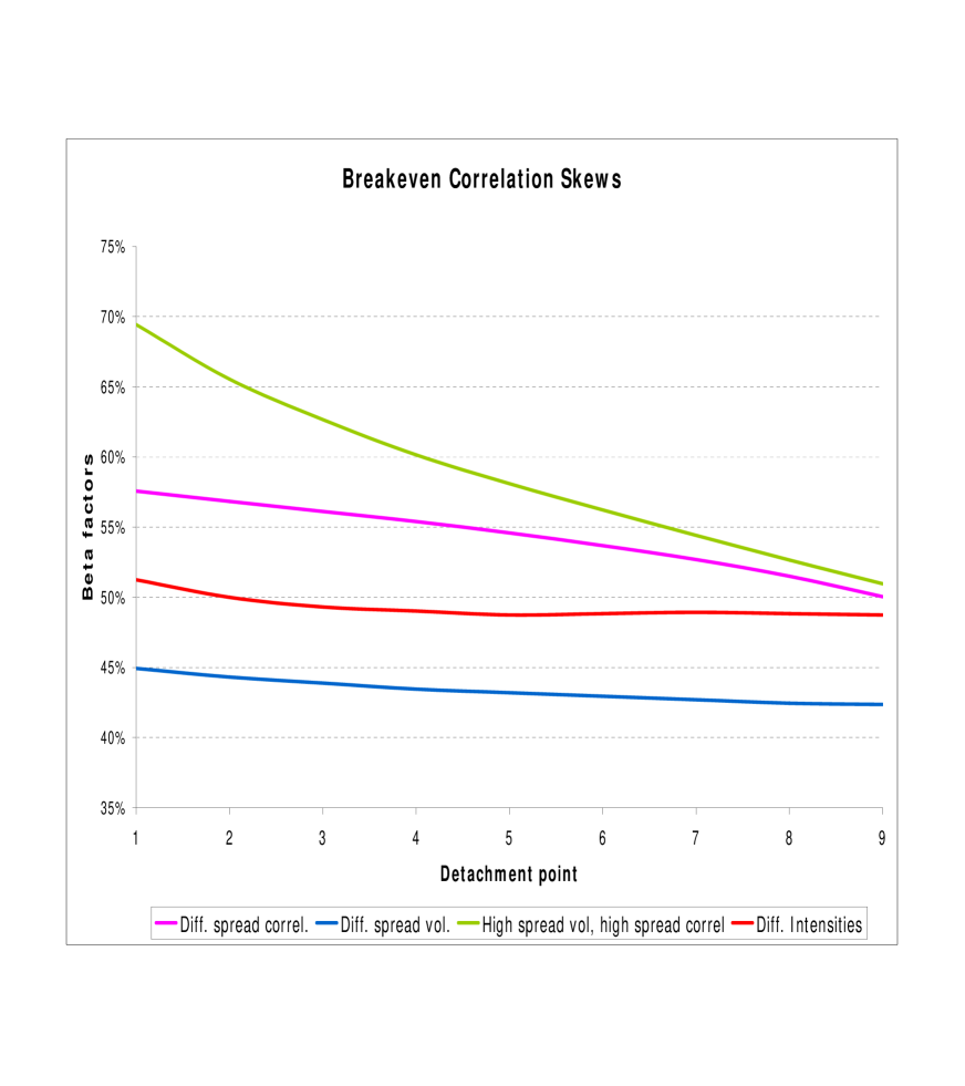
Figure 1: Break-even "beta factors" on a simulated trajectory

The reference case is related to a fully homogeneous basket, with default intensities of $\lambda_{0}=5\%$, constant volatilities of $\bar{\sigma}=50\%$ and constant spread correlations of $\rho_{ij}=50\%$ for all $i\neq j$. In this case, the "break-even beta factor"  is closed to $50\%$ and independent from the strike, as expected. Then, to move from this core scenario away, we have applied some deformations on these numbers: see tables 5, 6 and 7. Broadly speaking, these scenarii apply some rescaling method on all the parameters above, but differently from name to name. We observe different break-even correlation skews and smiles, depending on the heterogeneity of the underlying basket. For instance, in figure 1, different spread volatilities, spread correlations or initial default intensities per name (all other things being equal) generate downward sloping break-even correlations. This effect is more striking when high spread volatilities are associated with high spread correlations. Nonetheless, we can produce upward sloping break-even correlation skews by putting low beta factors on names that have got high intensities: figure 2. Note we get the opposite when the high beta factors are associated with high intensities. By combining these three dimensions, we can even generate some unexpected smiles/skews that are difficult to be forecasted: figure 3.

Name	Core	Up	Down
1	0.50	0.22	1.13
2	0.50	0.22	1.13
3	0.50	0.33	0.75
4	0.50	0.33	0.75
5	0.50	0.50	0.50
6	0.50	0.50	0.50
7	0.50	0.75	0.33
8	0.50	0.75	0.33
9	0.50	1.13	0.22
10	0.50	1.13	0.22

Table 5: Scenarii in terms of spread volatilities.

Name	Core	Up	Down
1	0.05	0.02	0.11
2	0.05	0.02	0.11
3	0.05	0.03	0.08
4	0.05	0.03	0.08
5	0.05	0.05	0.05
6	0.05	0.05	0.05
7	0.05	0.08	0.03
8	0.05	0.08	0.03
9	0.05	0.11	0.02
10	0.05	0.11	0.02

Table 6: Scenarii in terms of default intensities.

Name	Core	Up	Down
1	0.50	0.22	0.99
2	0.50	0.22	0.99
3	0.50	0.33	0.75
4	0.50	0.33	0.75
5	0.50	0.50	0.50
6	0.50	0.50	0.50
7	0.50	0.75	0.33
8	0.50	0.75	0.33
9	0.50	0.99	0.22
10	0.50	0.99	0.22

Table 7: Scenarii in terms of beta factors.

We have calculated historical series of Break-even correlations, on two standard credit indices: ITraxx S8 Master, and CDX IG9 Main, both between their launch in September 2007 and June 2009. In practice, we have calculated weekly P&Ls that are generated by continuously delta-hedging a base tranche $[0,x\%]$ (for ITraxx) or a senior tranche $[x\%,100\%]$ (for CDX). The hedging instruments are usual CDS on every name of the basket, and every relevant maturity. The CDO tranche calculation is led for a grid of constant correlation levels, from $0\%$ to $95\%$. We calculate P&L increments with a rolling window of six weeks. For every window, the (empirical) break-even correlation is the level of flat correlation that allows a zero P&L variation . Moreover, to simplify, we assume that no interest are generated in the cash account, and that the running premia of all the instruments (CDS and tranches) are zero. Thus, they are managed fully with upfront paiements.

For the sake of comparison, on our graphs, we have shown the break-even correlations and the associated base correlations, as deduced from the market: see figures 4, 5, 6, 7 for the CDX IG9 (main), and 8, 9, 10, 11, 12 for the index ITraxx S8 (main). It can be observed that the two series move consistently, even if the break-even series generate more volatile moves. But in average, the market base correlations are not so different from break-even ones, as expected, except for CDX senior tranches. It may be possible that investors in the latter tranches require an additional risk premium, or, in other words, overestimate systemic risk.

In this practical experiment, several factors move us from the theoretical framework away: the CDO tranches are not European , heterogeneity in terms of recovery rates for CDX, some default events have been observed during this period of time for CDX , and have not been fully anticipated by the market. Moreover, our base correlations depend on the BNP-Paribas current analytics that have evolved in this period of time . And, at the end of 2007, it has sometimes been difficult to find implied levels of base correlations from market quotes. Nonetheless, especially for ITraxx, it appears that the concept of Break-even correlation can be a very useful relative value tool. Indeed, theoretically, its moves should be in line with those of the market base correlations. It is what we observe empirically, broadly speaking. Thus, significant and persistent gaps between both types of correlations should help to forecast future moves of base correlations, because both series should converge towards each other finally.

9 Conclusion

We have shown under which conditions usual “static” credit portfolio models can be seen as replication models. Explicit expressions of dynamic hedging errors have been provided for a large class of portfolio derivatives. In particular, we have investigated the one factor Gaussian copula model, the market standard, and its multivariate extension. We have exhibited the unique family of dynamics (in terms of survival probabilities), that are consistent with a pricing by replication. We have shown that the matrix of spread correlations $\rho_{ij}$ and some spread “volatility-type” coefficients $\bar{\sigma}_{i}$ should be combined in a particular way to get break-even correlations. Broadly speaking, the matrix $[2\bar{\sigma}_{i}\bar{\sigma}_{j}\rho_{ij}/(\bar{\sigma}_{i}^{2}+\bar{\sigma}_{j}^{2})]$ should be definite positive. When it is the case, this matrix is our break-even correlation matrix and should be used for pricing and hedging purpose. We have shown that the one-factor copula is more tractable than most other factor models and why it is so difficult to find an alternative to it  by proving that most other models will not lend themselves to replication.

There remains a lot of avenues for further research. In particular, we should try to adapt our framework to deal with

1. richer dynamics in terms of survival probabilities, for instance by assuming underlying Levy processes,

2. random recoveries (Amraoui and Hitier 2008, Krekel 2008),

3. some extensions of the one-factor Gaussian copula framework, as random factor loadings (Andersen and Sidenius 2004) or local correlation (Turc et al. 2005),

4. perfect hedging when sudden jumps-to-default may occur before maturity.

5. joint specification of all the $Q_{it}(T)$-dynamics for different maturities $T$, i.e. an arbitrage-free specification of term structures.

All these points induce significant technical difficulties. Concerning the point (i), additional jumps components would challenge the desired perfect replication property. Moreover, random recoveries cannot be tackled easily. At first glance, it could be done by working with individual loss dynamics instead of survival probabilities $Q_{it}(T)$. In point (iii), the idea is to build a dependence between the pricing correlation level and the common factor, i.e. to price with some functions $\rho_{i}(x)$, $i=1,\ldots,n$. Point (iv) has been discussed in section 2. Since it should involve alternative sensitivities and alternative instruments, this task has been left for future research. The last point (v) is probably the most crucial one. All our analysis has been led with a given maturity $T$. With two maturities $T<T^{\prime}$ and the same framework, we can check that it is not possible to satisfy the arbitrage relation $Q_{it}(T)\geq Q_{it}(T^{\prime})$, for all times $t<T$. Indeed, when $t$ tends to $T$, $Q_{it}(T)$ will tend to zero with a certain probability, when $Q_{it}(T^{\prime})$ will not exhibit such a feature (as a consequence of the spread dynamics we have found). To find other model specifications, similar to first-hitting time models for instance, is the main challenge to tackle the multi-period formulation of the problem.

The authors thank their colleagues and former colleagues of BNP-Paribas and JP-Morgan for their help and fruitful discussions. Bruno Bouchard, Stéphane Crépey, Peter Jäckel, Monique Jeanbleanc, Jean-Paul Laurent, Dong Li and Marek Rutkowski have provided us highly valuable comments too.

Appendix A Proof of theorem 1

By the conditional independence property, the price of the structured product is

$$V_{t}=\sum_{\vec{\delta}(T)}\psi(\vec{\delta}(T))\int\displaystyle\prod_{j=1}^{n}p_{j|x}^{\delta_{j}}q_{j|x}^{1-\delta_{j}}f_{X}(x)\,dx=V(Q_{1},\ldots,Q_{n}),$$

with our notations. We have

$$\frac{\partial^{2}V_{t}}{\partial^{2}Q_{i}} =\sum_{\vec{\delta}(T)}\psi(\vec{\delta}(T))\int\displaystyle\prod_{j\neq i}p_{j|x}^{\delta_{j}}q_{j|x}^{1-\delta_{j}}.(2\delta_{i}-1)\frac{\partial^{2}p_{i|x}}{\partial^{2}Q_{i}}f_{X}(x)\,dx,$$ (33)

and, for every couple $(i,j)$, $i\neq j$,

$$\frac{\partial^{2}V_{t}}{\partial Q_{i}\partial Q_{j}} =\sum_{\vec{\delta}(T)}\psi(\vec{\delta}(T))\int\displaystyle\prod_{k\neq i,j}p_{k|x}^{\delta_{k}}q_{k|x}^{1-\delta_{k}}.(2\delta_{i}-1)(2\delta_{j}-1)\frac{\partial p_{i|x}}{\partial Q_{i}}\cdot\frac{\partial p_{j|x}}{\partial Q_{j}}f_{X}(x)\,dx.$$ (34)

Then, by applying Ito’s formula, we get

$$dV_{t} =(\ldots)\cdot d\vec{W}_{t}+\frac{1}{2}\sum_{i,j}\frac{\partial^{2}V_{t}}{\partial Q_{i}\partial Q_{j}}\sigma_{it}\sigma_{jt}\rho_{ij}dt$$

$$=(\ldots)\cdot d\vec{W}_{t}+\sum_{\vec{\delta}(T)}\psi(\vec{\delta}(T))\sum_{i=1}^{n}dt\int\displaystyle\prod_{j\neq i}p_{j|x}^{\delta_{j}}q_{j|x}^{1-\delta_{j}}.(2\delta_{i}-1)\frac{\sigma_{i}^{2}}{2}\cdot\frac{\partial^{2}p_{i|x}}{\partial^{2}Q_{i}}f_{X}(x)\,dx$$

$$+\frac{dt}{2}\sum_{i\neq j}\sum_{\vec{\delta}(T)}\psi(\vec{\delta}(T))\int\displaystyle\prod_{k\neq i,j}p_{k|x}^{\delta_{k}}q_{k|x}^{1-\delta_{k}}.(2\delta_{i}-1)(2\delta_{j}-1)\sigma_{i}\sigma_{j}\rho_{ij}\frac{\partial p_{i|x}}{\partial Q_{i}}\cdot\frac{\partial p_{j|x}}{\partial Q_{j}}f_{X}(x)\,dx$$

$$:=(\ldots)\cdot d\vec{W}_{t}+d\pi_{1}+d\pi_{2}.$$ (35)

By an integration by parts and with our notations, we get for every $i$

$$\int\displaystyle\prod_{j\neq i}p_{j|x}^{\delta_{j}}q_{j|x}^{1-\delta_{j}}\frac{\partial^{2}p_{i|x}}{\partial^{2}Q_{i}}f_{X}(x)\,dx$$

$$= \left[\displaystyle\prod_{j\neq i}p_{j|x}^{\delta_{j}}q_{j|x}^{1-\delta_{j}}\chi_{i}(x)\right]_{-\infty}^{+\infty}-\sum_{j,j\neq i}\int\displaystyle\prod_{k\neq i,j}p_{k|x}^{\delta_{k}}q_{k|x}^{1-\delta_{k}}.(2\delta_{j}-1)\frac{\partial p_{j|x}}{\partial x}\chi_{i}(x)\,dx.$$

We deduce

$$d\pi_{1} =\eta-\frac{dt}{2}\sum_{\vec{\delta}(T)}\psi(\vec{\delta}(T))\sum_{i<j}\int\displaystyle\prod_{k\neq i,j}p_{k|x}^{\delta_{k}}q_{k|x}^{1-\delta_{k}}.(2\delta_{i}-1)(2\delta_{j}-1)\left[\sigma_{i}^{2}\frac{\partial p_{j|x}}{\partial x}\chi_{i}(x)+\sigma_{j}^{2}\frac{\partial p_{i|x}}{\partial x}\chi_{j}(x)\right]\,dx,$$

and the formula follows. $\Box$

Appendix B Proof of equation (6)

To lighten the notations, set $\bar{s}_{j}:=\bar{\Phi}^{-1}(Q_{jt})$. Simple calculations provide

$$\frac{\partial p_{j|x}}{\partial Q_{j}}=-\frac{\phi(d_{j})}{\phi(\bar{s}_{j})\sqrt{1-\rho_{j}^{2}}},$$

and

$$\frac{\partial^{2}p_{j|x}}{\partial^{2}Q_{j}}=\frac{\phi(d_{j})}{\phi(\bar{s}_{j})^{2}(1-\rho_{j}^{2})^{3/2}}\rho_{j}[x-\rho_{j}\bar{\Phi}^{-1}(Q_{j})].$$

Thus,

$$\chi_{j}(x)=\frac{\rho_{j}}{\phi(\bar{s}_{j})^{2}(1-\rho_{j}^{2})^{3/2}}\int_{-\infty}^{x}[u-\rho_{j}\bar{s}_{j}].\phi(d_{j})\phi(u)\,du.$$

But a key point in favor of the Gaussian copula specification is that

$$\phi(d_{j})\phi(x)=\phi\left(\frac{x-\rho_{j}\bar{s}_{j}}{\sqrt{1-\rho_{j}^{2}}}\right)\phi(\bar{s}_{j}).$$ (36)

Therefore, we deduce

$$\chi_{j}(x) =\frac{\rho_{j}}{\phi(\bar{s}_{j})(1-\rho_{j}^{2})^{3/2}}\int_{-\infty}^{x}[u-\rho_{j}\bar{s}_{j}].\phi\left(\frac{u-\rho_{j}\bar{s}_{j}}{\sqrt{1-\rho_{j}^{2}}}\right)\,du$$

$$=-\frac{\rho_{j}\phi(d_{j})\phi(x)}{\phi(\bar{s}_{j})^{2}(1-\rho_{j}^{2})^{1/2}}=\frac{\rho_{j}\phi(x)}{\phi(\bar{s}_{j})}\cdot\frac{\partial p_{j|x}}{\partial Q_{j}}\cdot\hskip 85.35826pt$$

Moreover, we get easily

$$\frac{\partial p_{j|x}}{\partial x}=\rho_{j}\phi(\Phi^{-1}(Q_{jt}))\frac{\partial p_{j|x}}{\partial Q_{j}},$$

and the result follows from theorem 1.$\Box$

Appendix C Proof of theorem 4.

Clearly, conditions $(i)$, $(ii)$ and $(iii)$ are sufficient so that $(V_{t})$ is a ${{\mathcal{F}}}$-martingale under $Q$, invoking theorem 2.

Now, let us prove the necessity of such conditions. We want to cancel the drift of $dV_{t}$ for any random trajectory of all $(Q_{it})_{t\in I}$, $I\subset[0,T)$, $i=1,\ldots,n$. To fix the ideas and without a lack of generality, we consider the particular couple of indices $(1,2)$. In particular, the drift of $dV_{t}$ should be zero for trajectories where the $Q_{it}$ take very large or very small values, $i\neq 1,2$. To be specific, we will consider trajectories such that $\sup_{x}\phi(d_{i})\phi(x)<\varepsilon$, for a given $\varepsilon>0$, and when $i\neq 1,2$. Thus, since we are under the “no default” assumption, under our assumptions, the drift of $dV_{t}$ is

$$\frac{dt}{2}\left[2\beta_{1t}\beta_{2t}\rho_{12}-\rho_{1}\rho_{2}\beta_{1t}^{2}-\rho_{1}\rho_{2}\beta_{2t}^{2}\right]\sum_{\vec{\delta}(T)}\psi(\vec{\delta}(T))(2\delta_{1}-1)(2\delta_{2}-1)$$

$$\cdot\int\displaystyle\prod_{k\neq 1,2}p_{k|x}^{\delta_{k}}q_{k|x}^{1-\delta_{k}}\frac{\phi(d_{1})\phi(d_{2})\phi(x)}{\sqrt{1-\rho_{1}^{2}}\sqrt{1-\rho_{2}^{2}}}\,dx+O(\varepsilon).$$

We have assumed that there exist some indicators $\delta_{k}^{\ast}$, $k\neq 1,2$ such that

$$\psi(1,1,\vec{\delta}^{\ast}_{-(1,2)})-\psi(1,0,\vec{\delta}^{\ast}_{-(1,2)})-\psi(0,1,\vec{\delta}^{\ast}_{-(1,2)})+\psi(0,0,\vec{\delta}^{\ast}_{-(1,2)})\neq 0.$$

Now, consider a compact subset ${\cal A}$ such that $\int{\bf 1}(x\not\in{\cal A})\phi(x)\,dx<\varepsilon$. We can particularize our trajectories $Q_{it}$ even more, so that

• $$\sup_{x\in{\cal A}}\displaystyle\prod_{k\neq 1,2}p_{k|x}^{\delta_{k}}q_{k|x}^{1-\delta_{k}}\leq\varepsilon,$$

  when $\delta_{k}\neq\delta_{k}^{\ast}$ for at least one index $k\neq 1,2$, and

• $$\inf_{x\in{\cal A}}\displaystyle\prod_{k\neq 1,2}p_{k|x}^{\delta_{k}^{\ast}}q_{k|x}^{1-\delta_{k}^{\ast}}\geq 1/2.$$

This is possible, because, for every index $k\neq 1,2$, we can find $Q_{kt}$ such that $p_{k|x}$ (resp. $q_{k|x}$) is closed to one when $\delta_{k}^{\ast}=1$ ($\delta_{k}^{\ast}=0$), and uniformly w.r.t. $x$ in a compact subset.

Therefore, the sum defining the hedging error is “reduced” even more: for this particular choice of $Q_{kt}$, $k\neq i,j$, the drift of $dV_{t}$ is

$$\frac{dt}{2}\left(\psi(1,1,\vec{\delta}^{\ast}_{-(1,2)})-\psi(1,0,\vec{\delta}^{\ast}_{-(1,2)})-\psi(0,1,\vec{\delta}^{\ast}_{-(1,2)})+\psi(0,0,\vec{\delta}^{\ast}_{-(1,2)})\right)$$

$$\cdot\left[2\beta_{1t}\beta_{2t}\rho_{12}-\rho_{1}\rho_{2}\beta_{1t}^{2}-\rho_{1}\rho_{2}\beta_{2t}^{2}\right]\int\displaystyle\prod_{k\neq 1,2}p_{k|x}^{\delta^{\ast}_{k}}q_{k|x}^{1-\delta^{\ast}_{k}}\frac{\phi(d_{1})\phi(d_{2})\phi(x)}{\sqrt{1-\rho_{1}^{2}}\sqrt{1-\rho_{2}^{2}}}\,dx+O(\varepsilon)$$

$$=Cst\left[2\beta_{1t}\beta_{2t}\rho_{12}-\rho_{1}\rho_{2}\beta_{1t}^{2}-\rho_{1}\rho_{2}\beta_{2t}^{2}\right]\int_{{\cal A}}\phi(d_{1})\phi(d_{2})\phi(x)\,dx+O(\varepsilon).$$

Since $\varepsilon$ is arbitrarily small, this drift is zero if and only if

$$2\beta_{1t}\beta_{2t}\rho_{12}-\rho_{1}\rho_{2}[\beta_{1t}^{2}+\beta_{2t}^{2}]=0,$$

for every $Q_{1t}$ and $Q_{2t}$.

Actually, it is possible to lead the same reasoning for all couples $(i,j)$, $i\neq j$, under the assumption (P). Thus, we recover equation (4), that is now a necessary and sufficient condition:

$$2\beta_{it}\beta_{jt}\rho_{ij}=[\beta_{it}^{2}+\beta_{jt}^{2}]\rho_{i}\rho_{j},$$ (37)

for every $x$, $Q_{it}$, $Q_{jt}$ and every couple $(i,j)$, $i\neq j$. The latter condition can be true if and only if the previous $\beta_{it}$ are independent of $Q_{it}$. They can depend on time $t$, but iff $\beta_{it}/\beta_{jt}$ is independent of $t$ for all $(i,j)$, $i\neq j$. Therefore, we get equation (8), by rewriting $\beta_{it}$ as $\bar{\sigma}_{i}\xi_{t}$, for some positive function $\xi$ and some constant $\bar{\sigma}_{i}>0$. Our assumption on $\Sigma^{S}$ provides the existence of the pricing parameters $\rho_{i}$, $i=1,\ldots,n$.

To finish the proof, it remains to prove that $\lim_{t\rightarrow T}\int_{0}^{t}\xi_{u}^{2}\,du=+\infty$. By setting $Z_{t}=\Phi^{-1}(Q_{it})$ and invoking Ito’s lemma, we see easily that the solution of the PDE (8) is given by

$$Q_{it}=\Phi\left(\exp(\frac{\bar{\sigma}_{i}^{2}\int_{0}^{t}\xi_{u}^{2}\,du}{2})\Phi^{-1}(Q_{i0})+\int_{0}^{t}\exp(\frac{\bar{\sigma}_{i}^{2}\int_{u}^{t}\xi_{s}^{2}\,ds}{2})\bar{\sigma}_{i}\xi_{u}\,dW_{iu}\right),$$

where $(W_{iu})$ is a Brownian motion under $Q$. Note that $Q_{it}(T)$ tends to zero or one when $t$ tends to $T$. Assume that $\lim_{t\rightarrow T}\int_{0}^{t}\xi_{u}^{2}\,du=\ell<+\infty$. Then, $\int_{0}^{T}\exp(\bar{\sigma}_{i}^{2}\int_{u}^{T}\xi_{s}^{2}\,ds/2)\xi_{u}\,dW_{iu}$ is a non degenerate Gaussian r.v. and it will be impossible to get $\lim_{t\rightarrow T}Q_{it}\in\{0,1\}$ almost surely. So the result. $\Box$

Appendix D Proof of theorem 6.

We come back to the first steps of the proof of theorem 1 in section A. With these previous notations, we have now

$$\frac{d\pi_{1}}{dt}=\sum_{\vec{\delta}(T)}\psi(\vec{\delta}(T))\sum_{i=1}^{n}\int\displaystyle\prod_{j\neq i}p_{j|{\mathbf{x}}}^{\delta_{j}}q_{j|{\mathbf{x}}}^{1-\delta_{j}}.(2\delta_{i}-1)\frac{\sigma_{i}^{2}}{2}\cdot\frac{\partial^{2}p_{i|{\mathbf{x}}}}{\partial^{2}Q_{i}}f_{X}({\mathbf{x}})\,d{\mathbf{x}},$$ (38)

and

$$\frac{d\pi_{2}}{dt}=\frac{1}{2}\sum_{i\neq j}\sum_{\vec{\delta}(T)}\psi(\vec{\delta}(T))\int\displaystyle\prod_{k\neq i,j}p_{k|{\mathbf{x}}}^{\delta_{k}}q_{k|{\mathbf{x}}}^{1-\delta_{k}}.(2\delta_{i}-1)(2\delta_{j}-1)\sigma_{i}\sigma_{j}\rho_{ij}\frac{\partial p_{i|{\mathbf{x}}}}{\partial Q_{i}}\cdot\frac{\partial p_{j|{\mathbf{x}}}}{\partial Q_{j}}f_{X}({\mathbf{x}})\,d{\mathbf{x}}.$$ (39)

Under the $p$-factor Gaussian copula framework, these quantities can be rewritten:

$$\frac{d\pi_{1}}{dt}=\sum_{\vec{\delta}(T)}\psi(\vec{\delta}(T))\sum_{i=1}^{n}\int\displaystyle\prod_{j\neq i}p_{j|{\mathbf{x}}}^{\delta_{j}}q_{j|{\mathbf{x}}}^{1-\delta_{j}}.(2\delta_{i}-1)\frac{\sigma_{i}^{2}}{2}\cdot\frac{\phi(d_{i})[\rho_{i}^{\prime}{\mathbf{x}}-|\rho_{i}|^{2}\bar{s}_{i}]}{\phi(\bar{s}_{i})^{2}(1-|\rho_{i}|^{2})^{3/2}}\prod_{k=1}^{p}\phi(x_{k})\,dx_{k},$$ (40)

where, as previously, we have set $\bar{s}_{i}:=\bar{\Phi}^{-1}(Q_{it})$. Moreover,

$$\frac{d\pi_{2}}{dt}=\frac{1}{2}\sum_{i\neq j}\sum_{\vec{\delta}(T)}\psi(\vec{\delta}(T))\int\displaystyle\prod_{k\neq i,j}p_{k|{\mathbf{x}}}^{\delta_{k}}q_{k|{\mathbf{x}}}^{1-\delta_{k}}.(2\delta_{i}-1)(2\delta_{j}-1)$$ (41)

$$\cdot \sigma_{i}\sigma_{j}\rho_{ij}\frac{\phi(d_{i})\phi(d_{j})}{\phi(\bar{s}_{i})\phi(\bar{s}_{j})}\cdot\frac{\prod_{k=1}^{p}\phi(x_{k})\,dx_{k}}{\sqrt{1-|\rho_{i}|^{2}}\sqrt{1-|\rho_{j}|^{2}}}\cdot$$

The key point of the proof is to exhibit the right variables to make integration by parts. Let us introduce some additional notations : for any vector ${\mathbf{x}}$ in ${\mathbb{R}}^{p}$ and $r\in\{1,\ldots,p\}$, let us denote by ${\mathbf{x}}_{-r}$ the $p-1$ vector $(x_{1},\ldots,x_{r-1},x_{r+1},\ldots,x_{p})$. For every integer $r\leq p$, simple calculations provide the identity

$$\phi(d_{i})\phi(x_{r})=\phi\left(\sqrt{\frac{1-|\rho_{i,-r}|^{2}}{1-|\rho_{i}|^{2}}}\cdot\{x_{r}-\frac{\rho_{i,r}\bar{s}_{i,r}}{1-|\rho_{i,-r}|^{2}}\}\right)\cdot\phi\left(\frac{\bar{s}_{i,r}}{\sqrt{1-|\rho_{i,-r}|^{2}}}\right),$$ (42)

where $\bar{s}_{i,r}=\bar{s}_{i}-\rho_{i,-r}^{\prime}{\mathbf{x}}_{-r}$. Now, it can be checked that we can rewrite

$$\rho_{i}^{\prime}{\mathbf{x}}-|\rho_{i}|^{2}\bar{s}_{i}=\sum_{r=1}^{p}\left[\rho_{ir}x_{r}(1-|\rho_{i,-r}|^{2})-c_{ir}\right],$$

where we have set

$$c_{ir}:=\rho_{ir}^{2}\bar{s}_{i}-\rho_{ir}^{2}\rho_{i,-r}^{\prime}{\mathbf{x}}_{-r}.$$

We deduce $d\pi_{1}=\sum_{r=1}^{p}d\pi_{1,r},$ with

$$\frac{d\pi_{1,r}}{dt}=\sum_{\vec{\delta}(T)}\psi(\vec{\delta}(T))\sum_{i=1}^{n}\int\displaystyle\prod_{j\neq i}p_{j|{\mathbf{x}}}^{\delta_{j}}q_{j|{\mathbf{x}}}^{1-\delta_{j}}.(2\delta_{i}-1)\frac{\sigma_{i}^{2}}{2}\cdot\frac{\phi(d_{i})[\rho_{ir}x_{r}(1-|\rho_{i,-r}|^{2})-c_{ir}]}{\phi(\bar{s}_{i})^{2}(1-|\rho_{i}|^{2})^{3/2}}\prod_{k=1}^{p}\phi(x_{k})\,dx_{k}.$$

But, by integrating w.r.t. the variable $x_{r}$ and by invoking equation (42), we observe that

$$\int_{-\infty}^{x_{r}}\phi(d_{i})[\rho_{ir}u_{r}(1-|\rho_{i,-r}|^{2})-c_{ir}]\phi(x_{r})\,du_{r}$$

$$= -\rho_{ir}(1-|\rho_{i}|^{2})\phi\left(\sqrt{\frac{1-|\rho_{i,-r}|^{2}}{1-|\rho_{i}|^{2}}}\cdot\{x_{r}-\frac{\rho_{i,r}\bar{s}_{i,r}}{1-|\rho_{i,-r}|^{2}}\}\right)\cdot\phi\left(\frac{\bar{s}_{i,r}}{\sqrt{1-|\rho_{i,-r}|^{2}}}\right)$$

$$= -\rho_{ir}(1-|\rho_{i}|^{2})\phi(d_{i})\phi(x_{r}).$$

Thus, by an integration by parts w.r.t. $x_{r}$, we get

$$\frac{d\pi_{1,r}}{dt}=-\sum_{\vec{\delta}(T)}\psi(\vec{\delta}(T))\sum_{i=1}^{n}\sum_{j\neq i}\int\displaystyle\prod_{k\neq i,j}p_{k|{\mathbf{x}}}^{\delta_{j}}q_{k|{\mathbf{x}}}^{1-\delta_{j}}.(2\delta_{i}-1)(2\delta_{j}-1)\frac{\sigma_{i}^{2}}{2}\cdot\frac{\partial p_{j|{\mathbf{x}}}}{\partial x_{r}}$$

$$\cdot \frac{\rho_{ir}(1-|\rho_{i}|^{2})\phi(d_{i})}{\phi(\bar{s}_{i})^{2}(1-|\rho_{i}|^{2})^{3/2}}\prod_{k=1}^{p}\phi(x_{k})\,dx_{k}$$

$$= -\sum_{\vec{\delta}(T)}\psi(\vec{\delta}(T))\sum_{i\neq j}\int\displaystyle\prod_{k\neq i,j}p_{k|{\mathbf{x}}}^{\delta_{j}}q_{k|{\mathbf{x}}}^{1-\delta_{j}}.(2\delta_{i}-1)(2\delta_{j}-1)\frac{\sigma_{i}^{2}}{2}$$

$$\cdot \frac{\rho_{ir}\rho_{jr}\phi(d_{i})\phi(d_{j})}{\phi(\bar{s}_{i})^{2}(1-|\rho_{i}|^{2})^{1/2}(1-|\rho_{j}|^{2})^{1/2}}\prod_{k=1}^{p}\phi(x_{k})\,dx_{k}.$$

And then, by summing up on $r$, we obtain

$$\frac{d\pi_{1}}{dt}=-\sum_{\vec{\delta}(T)}\psi(\vec{\delta}(T))\sum_{i<j}\int\displaystyle\prod_{k\neq i,j}p_{k|{\mathbf{x}}}^{\delta_{j}}q_{k|{\mathbf{x}}}^{1-\delta_{j}}$$ (43)

$$\cdot \frac{(2\delta_{i}-1)(2\delta_{j}-1)\phi(d_{i})\phi(d_{j})}{2(1-|\rho_{i}|^{2})^{1/2}(1-|\rho_{j}|^{2})^{1/2}}\rho_{i}^{\prime}\rho_{j}[\frac{\sigma_{i}^{2}}{\phi(\bar{s}_{i})^{2}}+\frac{\sigma_{j}^{2}}{\phi(\bar{s}_{j})^{2}}]\prod_{k=1}^{p}\phi(x_{k})\,dx_{k}.\hskip 85.35826pt$$

By summing the equations (43) and (41) up, we get the result. $\Box$

Appendix E Proof of theorem 10.

Let $\psi_{p}(\vec{\delta})=\min(\sum_{i=1}^{n}\delta_{i},p).(1-R),$ and $\theta_{p}(\vec{\delta})={\bf 1}(\sum_{i=1}^{n}\delta_{i}\leq p).(1-R)$. We can checked easily that, for every $p\geq 1$,

$$\psi_{p}=\psi_{p-1}+1-R-\theta_{p-1}.$$

The drift of the value process associated with a particular payoff $\psi$ will be denoted by $d\pi(\psi)$. Obviously, $\pi$ is a linear functional, and $d\pi(\psi)=0$ if the payoff is risk-free. We deduce

$$d\pi(\psi_{p})=d\pi(\psi_{p-1})-d\pi(\theta_{p-1}).$$ (44)

Now, let us specify $d\pi(\theta_{p})$ for $p\leq n$. To lighten the notations, we set

$$\tilde{A}_{ij}=\frac{(1-R)}{2}\left[2\beta_{it}\beta_{jt}\rho_{ij}-\rho_{i}\rho_{j}\beta_{it}^{2}-\rho_{i}\rho_{j}\beta_{jt}^{2}\right]\frac{\phi(d_{i})\phi(d_{j})\phi(x)}{\sqrt{1-\rho_{i}^{2}}\sqrt{1-\rho_{j}^{2}}}\cdot$$

Let us apply theorem 2. By distinguishing between the different values that are taken by the couples $(\delta_{i},\delta_{j})$, we get

$$d\pi_{t}(\theta_{p})=\sum_{\vec{\delta}(T)}{\bf 1}(\sum_{l=1}^{n}\delta_{l}\leq p)\sum_{i<j}(2\delta_{i}-1).(2\delta_{j}-1)\int\displaystyle\prod_{k\neq i,j}p_{k|x}^{\delta_{k}}q_{k|x}^{1-\delta_{k}}\tilde{A}_{ij}\,dx\,dt$$

$$= \sum_{i<j}\sum_{\vec{\delta}_{-(i,j)}}\left[{\bf 1}(\sum_{l\neq i,j}\delta_{l}\leq p-2)-2{\bf 1}(\sum_{l\neq i,j}\delta_{l}\leq p-1)+{\bf 1}(\sum_{l\neq i,j}\delta_{l}\leq p)\right]\cdot\int\displaystyle\prod_{k\neq i,j}p_{k|x}^{\delta_{k}}q_{k|x}^{1-\delta_{k}}\tilde{A}_{ij}\,dx\,dt,$$

where $\vec{\delta}_{-(i,j)}$ denotes the vector of $(\delta_{k})$, with $k\in\{1,\ldots,n\}$ but $k\neq i,j$. To simplify, let us denote

$$\alpha_{p}:=\sum_{i<j}\sum_{\vec{\delta}_{-(i,j)}}{\bf 1}(\sum_{l\neq i,j}\delta_{l}=p)\int\displaystyle\prod_{k\neq i,j}p_{k|x}^{\delta_{k}}q_{k|x}^{1-\delta_{k}}\tilde{A}_{ij}\,dx\,dt.$$

If $p\geq 1$, we have got

$$d\pi_{t}(\theta_{p}) =\sum_{i<j}\sum_{\vec{\delta}_{-(i,j)}}[{\bf 1}(\sum_{l\neq i,j}\delta_{l}=p)-{\bf 1}(\sum_{l\neq i,j}\delta_{l}=p-1)]\int\displaystyle\prod_{k\neq i,j}p_{k|x}^{\delta_{k}}q_{k|x}^{1-\delta_{k}}\tilde{A}_{ij}\,dx\,dt,$$

$$=\alpha_{p}-\alpha_{p-1}.$$

We deduce, for all $p\geq 2$,

$$d\pi(\psi_{p})=d\pi(\psi_{p-1})-\alpha_{p-1}+\alpha_{p-2}.$$

By iterating the latter equation, we get $d\pi(\psi_{p})=d\pi(\psi_{1})-\alpha_{p-1}+\alpha_{0}$. But $\pi(\psi_{1})$ is the hedging error of the First To Default, that is equal to $-\alpha_{0}$ (see equation (14)). Finally, we get $d\pi(\psi_{p})=-\alpha_{p-1},$ so the result. $\Box$

Appendix F Proof of theorem 11

In the one-period Merton model, with our notations and given ${\cal H}_{t}$,

$$p_{j,t|x} =Q\left(\tau_{j}\leq T|{\cal H}_{t}\right)=Q\left(\int_{0}^{T}\psi_{j}(u)\,dW_{ju}<\bar{b}_{jT}|{\cal H}_{t}\right)$$

$$=Q\left(\sqrt{1-\rho_{j}^{2}}\int_{t}^{T}\psi_{j}(u)\,dW^{\ast}_{ju}<\bar{b}_{jT}-\int_{0}^{t}\psi_{j}(u)\,dW_{ju}-\rho_{j}\int_{t}^{T}\psi_{j}(u)\,dW_{u}|{\cal H}_{t}\right)$$

$$=\Phi\left(\frac{\bar{b}_{jT}-\int_{0}^{t}\psi_{j}(u)\,dW_{ju}-\rho_{j}\int_{t}^{T}\psi_{j}(u)\,dW_{u}}{\sqrt{1-\rho_{j}^{2}}\sqrt{T-t}}\right):=\Phi(d_{jt}^{*}).$$

When $\psi_{j}(u)=1$ for any $j$ and $u$, we recover the standard Merton model and the pricing formula (5). In this case, ${\cal H}_{t}=\sigma(W_{ju},W_{T}-W_{u},u\leq t)$. For any $t,t^{\prime}$, $T\geq t>t^{\prime}\geq 0$, we get

$$E[p_{j,t|x}|{\cal H}_{t^{\prime}}]=E\left[\Phi\left(\frac{\bar{b}_{jT}-W_{jt}-\rho_{j}(W_{T}-W_{t})}{\sqrt{1-\rho_{j}^{2}}\sqrt{T-t}}\right)|{\cal H}_{t^{\prime}}\right]$$

$$= E\left[{\bf 1}\left(\sqrt{1-\rho_{j}^{2}}\sqrt{T-t}Z+(W_{jt}-W_{jt^{\prime}})-\rho_{j}(W_{t}-W_{t^{\prime}})\leq\bar{b}_{jT}-W_{jt^{\prime}}-\rho_{j}(W_{T}-W_{t^{\prime}})\right)|{\cal H}_{t^{\prime}}\right]$$

$$= E\left[{\bf 1}\left(\sqrt{1-\rho_{j}^{2}}\sqrt{T-t}Z+\sqrt{1-\rho_{j}^{2}}(W^{*}_{jt}-W^{*}_{jt^{\prime}})\leq\bar{b}_{jT}-W_{jt^{\prime}}-\rho_{j}(W_{T}-W_{t^{\prime}})\right)|{\cal H}_{t^{\prime}}\right],$$

for some gaussian r.v. $Z$, independent of $(W_{jt})$ and $(W_{t})$. We get

$$E[p_{j,t|x}|{\cal H}_{t^{\prime}}]=\Phi\left(\frac{\bar{b}_{jT}-W_{it^{\prime}}-\rho_{j}(W_{T}-W_{t^{\prime}})}{\sqrt{1-\rho_{j}^{2}}\sqrt{T-t^{\prime}}}\right)=p_{j,t^{\prime}|x}.$$

Therefore, the process $(p_{jt|x=W_{T}-W_{t}})_{t\in[0,T]}$ is an ${\cal H}$-martingale under $Q$. $\Box$

Appendix G Proof of theorem 12

In an Archimedean framework, we would like to find some dynamics that allow a cancellation of the hedging error $d\pi_{t}$ over all trajectories $(Q_{it})$, $i=1,\ldots,n$, $t\in[0,T]$ and for all payoff $\psi$. It implies we have to satisfy equation (4) by the same arguments as in the proof of theorem C. Particularly, we assume the case $Q_{it}=Q_{jt}$ for all $t$ and for some couple $(i,j)$, $i\neq j$  Since the volatilities are the same measurable functions of their trajectories $(Q_{it})$, this implies that $\sigma_{it}=\sigma_{jt}$ on these particular trajectories. Thus, we have to satisfy the necessary relation

$$a\left(\frac{\partial p_{i|x}}{\partial Q_{i}}\right)^{2}f_{X}(x)=\chi_{i}(x)\frac{\partial p_{i|x}}{\partial x}$$ (45)

for some non zero constant $a$. By simple calculations, it is equivalent to

$$ax^{2}p_{i|x}f_{X}(x)=\left[\xi^{\prime}(\bar{\xi}_{i})\right]^{2}\bar{\xi}_{i}\chi_{i}(x),$$

for all $x$ in the support of $X$ and every $Q_{i}\in[0,1]$. By deriving w.r.t $x$ and by making the change of variable $y=\bar{\xi}_{i}$, we have to satisfy

$$a[2-yx+x\frac{f_{X}^{\prime}}{f_{X}}(x)]=y[x+\frac{\xi^{\prime\prime}}{\xi^{\prime}}(y)],$$ (46)

for all $x$ in the support of $f_{X}$ and for all $y\in[0,1]$. Particularly, when $y$ tends to zero, $\frac{\xi^{\prime\prime}}{\xi^{\prime}}(y)$ tends to $-E[X^{2}]/E[X]$ that is finite by assumption. Thus, we have to satisfy

$$x\frac{f_{X}^{\prime}}{f_{X}}(x)+2=0,$$

for all $x\geq 0$. This implies the support of the density function $f_{X}$ contains some interval $[\alpha,\beta]\subset{\mathbb{R}}^{+}$, where it is equal to

$$f_{X}(x)=\frac{\alpha}{x^{2}},$$

for some positive constant $\alpha$. But then, equation (46) implies $a=(-1)$ and $\xi^{\prime\prime}=0$, that cannot be satisfied clearly. $\Box$

Appendix H Proof of theorem 13

Under our assumptions, we calculate

$$\frac{\partial p_{i|x}}{\partial Q_{i}}=-x\theta p_{i|x}(1-Q_{it})^{-\theta-1},$$

$$\frac{\partial^{2}p_{i|x}}{\partial^{2}Q_{i}}=(x\theta)^{2}p_{i|x}(1-Q_{it})^{-2\theta-2}-x\theta(\theta+1)p_{i|x}(1-Q_{it})^{-\theta-2},$$

$$\frac{\partial p_{i|x}}{\partial x}=p_{i|x}[1-(1-Q_{it})^{-\theta}].$$

By an integration by part, we obtain the identity

$$\chi_{i}(x)=\frac{\partial p_{i|x}}{\partial Q_{i}}\cdot\frac{x\theta f_{X}(x)}{1-Q_{it}}\cdot$$

Therefore, with our choices of volatilities $\sigma_{it}$ and the underlying processes, it can be checked easily we satisfy (4), replacing $\rho_{ij}$ by

$$<dQ_{it},dQ_{jt}>=\sigma_{it}\sigma_{jt}\beta_{i}^{\prime}(Q_{it})\beta_{j}(Q_{jt}).$$

Finally, we do not have to take into account the so-called term $\eta$ of the theorem 1, because $\lim_{x\rightarrow 0}\chi_{i}(x)=0$ and $\lim_{x\rightarrow+\infty}\chi_{i}(x)=0$. $\Box$

Appendix I Proof of theorem 14

To lighten the notations, we set $\eta_{i}:=\eta\left(\alpha_{i}x-h(Q_{it})\right)$, $h_{i}:=h(Q_{it})$ and $f:=f_{X}(x)$. Under our assumptions, we get easily

$$\frac{\partial p_{i|x}}{\partial x}=\eta_{i}^{\prime}\alpha_{i},\;\;\frac{\partial p_{i|x}}{\partial Q_{i}}:=-\eta_{i}^{\prime}h^{\prime}_{i},\;\;\frac{\partial^{2}p_{i|x}}{\partial^{2}Q_{i}}:=\eta_{i}^{\prime\prime}(h^{\prime}_{i})^{2}-\eta_{i}^{\prime}h^{\prime\prime}_{i}.$$

We would like to satisfy the partial differential equation (4) that is rewritten here

$$2(\sigma_{i}h^{\prime}_{i}).(\sigma_{j}h^{\prime}_{j})\rho_{ij}f=\alpha_{j}\sigma_{i}^{2}\frac{\chi_{i}}{\eta^{\prime}_{i}}+\alpha_{i}\sigma_{j}^{2}\frac{\chi_{j}}{\eta^{\prime}_{j}}\cdot$$ (47)

The latter equation has to be satisfied for all the triplets $(Q_{i},Q_{j},x)$. Actually, it is a very strong constraint, because it can be proved that this implies: there exist some constants $C_{i}$ and $\bar{C}(i,j)$, $i,j=1,\ldots,n$, such that

$$\sigma_{i}h^{\prime}_{i} = C_{i},$$ (48)

$$\sigma_{i}^{2}\frac{\chi_{i}}{\psi^{\prime}_{i}}\alpha_{j} = \bar{C}(i,j)\rho_{ij}f,$$ (49)

for all indices $(i,j)$, $i\neq j$. The latter result is a consequence of the following lemma:

Lemma. 15

Consider some real functions $a,b,c,d$ such that

$$a(x)b(y)=c(x)+d(y),$$

for all couples $(x,y)$. Then these four functions are constant.

This lemma is proved at the end of the current proof. Note that $C_{i}$ is not a function of $x$ because $\sigma h^{\prime}_{i}$ is a function of $Q_{i}$ only (not of $x$). Moreover, equation (49) is due to the fact we can consider the particular case $\alpha_{i}=\alpha_{j}$ and some trajectories where $Q_{it}=Q_{jt}$ .

From the latter equations, we get the existence of a constant $\mu=\mu(i,j)$ such that

$$\chi_{i}=\mu f\eta^{\prime}_{i}(h^{\prime}_{i})^{2}.$$

By differentiating this equation w.r.t. $x$, we get

$$\frac{\eta^{\prime\prime}_{i}}{\eta^{\prime}_{i}}-\frac{h^{\prime\prime}_{i}}{(h^{\prime}_{i})^{2}}=\mu\left[\frac{f^{\prime}}{f}+\alpha_{i}\frac{\eta^{\prime\prime}_{i}}{\eta^{\prime}_{i}}\right].$$ (50)

Now, by integrating the latter equation w.r.t. $x$, we obtain

$$\eta^{\prime}_{i}=\exp\left(\nu_{i}+\frac{xh^{\prime\prime}_{i}}{(1-\mu\alpha_{i})(h^{\prime}_{i})^{2}}\right)f^{\mu/(1-\mu\alpha_{i})},$$ (51)

for some function $\nu_{i}:=\nu(Q_{i})$. But (50) can be multiplied by $h^{\prime}_{i}$. And after an integration w.r.t. $Q_{i}$, we get

$$\eta^{\prime}_{i}=\exp\left(\xi(x)-\frac{[\ln(h^{\prime}_{i})+\mu_{i}f^{\prime}h_{i}/f]}{(1-\mu\alpha_{i})}\right),$$ (52)

for some function $\xi$. If $f^{\prime}/f$ were a constant function, the density $f$ would be exponentially distributed and the support of $X$ cannot be ${\mathbb{R}}$ as a whole. Moreover, $h$ is a not a constant by assumption. Thus, equations (51) and (52) together imply that the crossed terms $f^{\prime}h_{i}/f$ and $xh^{\prime\prime}_{i}(h^{\prime}_{i})^{-2}$ are proportional. In other words, this means that $f^{\prime}/f$ (resp. $h_{i}h^{\prime}_{i}$) is proportional to $x$ (resp. $h^{\prime\prime}_{i}/h^{\prime}_{i}$). Therefore, by integration, we check that the usual Gaussian copula model is the single possible model that satisfies such requirements. $\Box$

To finalize this proof, it remains to state lemma 15. This is done now.

If there exists some real number $x$ such that $a(x)=0$, then it is clear that $c$ and $d$ are constant functions, and then $a$ and $b$ too. We can lead the same reasoning with $b$. Thus, we can assume that $a$ and $b$ cannot be zero. Now, assume that $b$ is not a constant: there exist a couple $(y_{1},y_{2})$ such that $b(y_{1})\neq b(y_{2})\neq 0$. Then, for every real number $x$, we have

$$\frac{b(y_{1})}{b(y_{2})}=\frac{c(x)+d(y_{1})}{c(x)+d(y_{2})},$$

that is constant function in $x$. This implies that $c$ is a constant function of $x$, and that $d=\alpha b+\beta$ for some constants $\alpha$ and $\beta$. We deduce that $a(x)=(c+\alpha b(y)+\beta)/b(y)$, so $a$ and $b$ are constant functions.

This is a contradiction with our initial assumption. Since this reasoning can be lead with $a$ instead of $b$ similarly, we have proved our lemma. $\Box$

Figure 2: Break-even "beta factors" on a simulated trajectory

Figure 3: Break-even "beta factors" on a simulated trajectory

Figure 4: Break-even correlations and base correlations, CDX IG9, $3\%-100\%$.

Figure 5: Break-even correlations and base correlations, CDX IG9, $7\%-100\%$.

Figure 6: Break-even correlations and base correlations, CDX IG9, $10\%-100\%$.

Figure 7: Break-even correlations and base correlations, CDX IG9, $15\%-100\%$.

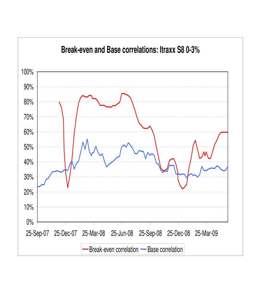
Figure 8: Break-even correlations and base correlations, ITraxx Main S8, $0-3\%$.

Figure 9: Break-even correlations and base correlations, ITraxx Main S8, $0-6\%$.

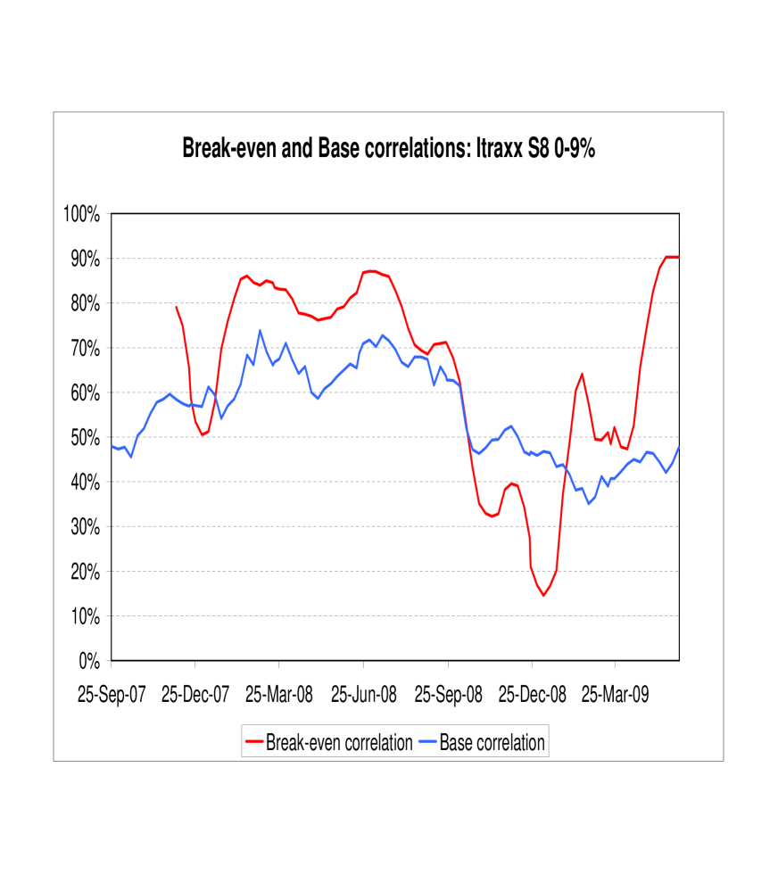
Figure 10: Break-even correlations and base correlations, ITraxx Main S8, $0-9\%$.

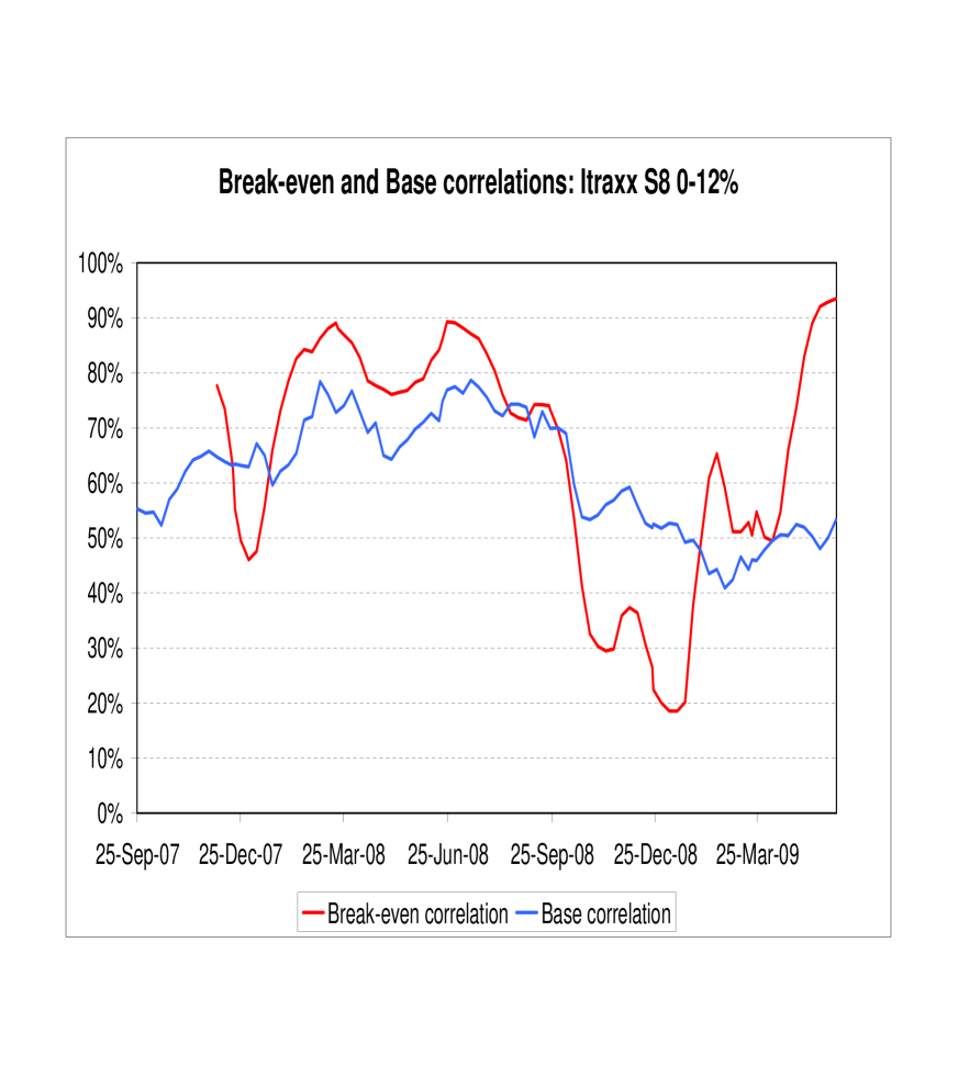
Figure 11: Break-even correlations and base correlations, ITraxx Main S8, $0-12\%$.

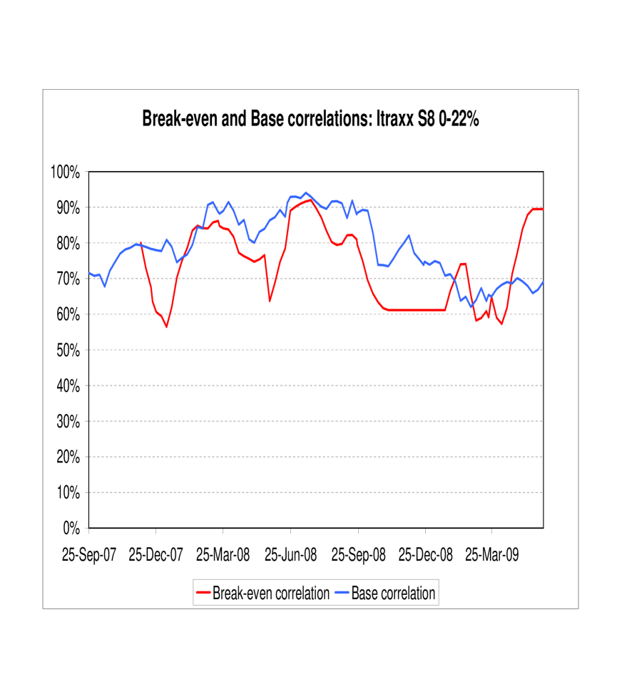
Figure 12: Break-even correlations and base correlations, ITraxx Main S8, $0-22\%$.

References

• [1] Ammann, M. and Brommundt, B. (2009): Hedging Collateralized Debt Obligations. Working paper, University of St Gallen.
• [2] Amraoui, S. and Hitier, S. (2008): Optimal stochastic recovery for base correlation. Working paper.
• [3] Andersen, L. and Sidenius, J. (2004): Extensions to the Gaussian copula: random recovery and random factor loadings. J. Credit Risk, 1, Vol. 1, $29-70$.
• [4] M. Arnsdorf and I. Halperin (2008): BSLP: Markovian bivariate spread-loss model for porfolio credit dervatives. Journal of Computational Finance, 12.
• [5] BNP-Paribas (2007): Inside Break-Even Correlation. Structured Credit Strategy Report, 31 October 2007.
• [6] T.R. Bielecki & Rutkowski, M. (2002): Credit Risk: Modeling, Valuation and Hedging. Springer.
• [7] Brasch, H-J. (2006): Exact replication of $k$-th-to-default with First-to-default swaps. Working paper, Rabobank.
• [8] Brigo, D. and Alfonsi, A. (2005): Credit Default Swaps calibration and option pricing with the SSRD stochastic intensity and interest-rate model. Finance & Stochastics., 9, $29-42$.
• [9] Burtschell, B., Gregory J. and Laurent, J-P. (2005): A comparative analysis of CDO pricing models. In The Definitive Guide to CDOs, G. Meisner (ed), Chapter 17, $461-480$, Risk Books.
• [10] Carr, P. & Madan, D. (2001): Towards a Theory of Volatility Trading. In Advances in Mathematical Finance. Eds. J. Cvitanic, E. Jouini and M. Musiela. Cambridge University Press.
• [11] Cont, R. and Kan, Y.H. (2008): Dynamic Hedging of Portfolio Credit Derivatives, Financial Engineering Report 2008-08, Columbia University.
• [12] Cont, R., Deguest, R. and Kan, Y. H. (2010): Recovering Default Intensity from CDO Spreads: Inversion Formula and Model Calibration, SIAM Journal on Financial Mathematics, 1, 555-585.
• [13] Cousin, A. and Jeanblanc, M. (2010): Hedging portfolio loss derivatives with CDSs. Working paper.
• [14] Cousin, A., Jeanblanc, M. and Laurent, J.-P. (2010): Hedging CDO tranches in a Markovian environment, Forthcoming in Paris-Princeton Lectures in Mathematical Finance, Lecture Notes in Mathematics, Springer.
• [15] Cousin, A., Crepey, S. and Kan, Y.H. (2010): Delta-hedging Correlation Risk? Working paper.
• [16] Duffie, D. & Garleanu, N. (2001): Risk and Valuation of Collateralized Debt Obligations. Financial Analysts Journal, 57, Number 1 (January-February), $41-59$.
• [17] Frey, R. and Backhaus, J. (2009): Dynamic hedging of synthetic CDO-tranches with spread and contagion risk, Forthcoming in Journal of Economic Dynamics and Control.
• [18] Frey, R. and Backhaus, J. (2008): Pricing and hedging of portfolio credit derivatives with interacting default intensities. International Journal of Theoretical and Applied Finance, 11, 611-634.
• [19] Garcia J., Goossens, S., Masol, V. & Schoutens, W. (2007). Lévy Base Correlation. Working paper.
• [20] Hull, J. and White, A. (2003): The valuation of credit default swap options. J. Derivatives, 10(3), $40-50$.
• [21] Hull, J. Predescu, M. and White, A. (2006): The valuation of correlation- dependent credit derivatives using a structural model. Journal of Credit Risk, forthcoming.
• [22] Jaeckel, P. (2008). The Discrete Gamma Pool model. Working paper.
• [23] Joshi, M. & A. Stacey (2005): Intensity Gamma: A new approach to pricing portfolio credit derivatives. Working paper.
• [24] Herbertsson, A. (2008): Pricing Synthetic CDO Tranches in a Model with Default Contagion using the Matrix-Analytic Approach. Journal of Credit Risk, 4, $335$.
• [25] Krekel, M. (2008): Pricing distressed CDOs with base correlation and stochastic recovery. Working paper.
• [26] Laurent, J-P. & Gregory, J. (2005): Basket default swaps, CDOs and factor copulas. Journal of Risk, 7, 4, $103-122$.
• [27] Laurent, J.-P., Cousin, A. and Fermanian, J-D. (2008): Hedging default risks of CDOs in Markovian contagion models. Forthcoming in Quantitative Finance.
• [28] Li, D. (2000): On default correlation: A copula function approach. J. Fixed Income, 9, $43-54$.
• [29] Lipton, A. and Rennie, A. (ed.) (2008): Credit correlation. Life after copulas. World Scientific.
• [30] Merton, R. (1974): On the pricing of corporate debt: the risk structure of interest rates. J. of Finance, $\rm 29$, $449-470$.
• [31] O’Kane, D. and Livasey, M. (2004): Base Correlation Explained. Quantative Credit Research. Lehman Brothers. Vol. 2004-Q3/4
• [32] Singpurwalla, N. & Youngren, M. (1993): Multivariate Distributions Induced by Dynamic Environments. Scand. J. Statistics, 20, $251-261$.
• [33] Turc, J., Very, P. and Benhamou D. (2005): Pricing CDOs with a smile. Société Générale, Credit Research. Feb.
• [34] Zhou, C. (2001): An analysis of default correlations and mutiples defaults. Review Financial Studies, 14, $555-576$.