X-ray Phase-Resolved Spectroscopy of PSRs B0531+21, B1509-58, and B0540-69 with RXTE

Abstract

The Rossi X-ray Timing Explorer (RXTE) has made hundreds of observations on three famous young pulsars (PSRs) B0531+21 (Crab), B1509-58, and B0540-69. Using the archive RXTE data, we have studied the phase-resolved spectral properties of these pulsars in details. The variation of the X-ray spectrum with phase of PSR B0531+21 is confirmed here much more precisely and more details are revealed than the previous studies: the spectrum softens from the beginning of the first pulse, turns to harden right at the pulse peak and becomes the hardest at the bottom of the bridge, softens gradually until the second peak, and then softens rapidly. Different from the previous studies, we found that the spectrum of PSR B1509-58 is significantly harder in the center of the pulse, which is also in contrast to that of PSR B0531+21. The variation of the X-ray spectrum of PSR B0540-69 seems similar to that of PSR B1509-58, but with a lower significance. Using the about 10 years of data span, we also studied the real time evolution of the spectra of these pulsars, and no significant evolution has been detected. We have discussed about the constraints of these results on theoretical models of pulsar X-ray emission.

1 Introduction

Phase resolved X-ray spectroscopy is very important for the verification of pulsar emission models. Currently there are two kinds of popular models to interpret the high energy emission of pulsars: the polar gap model and the outer gap model. The polar gap models assume that primary charged articles are accelerated above the neutron star surface and the $\gamma$-rays result from a curvature radiation and inverse Compton induced pair cascade in a strong magnetic field (Sturner & Dermer, 1994; Daugherty & Harding, 1996). The radiated spectra from these cascades are hard with photon indices 1.5-2.0 (Harding & Daugherty, 1998). Outer gap models (Cheng, Ho & Ruderman, 1986a, b; Romani, 1996) assume that acceleration occurs along null charge surfaces in the outer magnetosphere and that $\gamma$-rays result from photon-photon pair-production-induced cascade. Cheng et al. (2000) (hereafter CRZ model) have re-considered the three-dimensional magnetosphere gap model by introducing various physical processes (including pair production, surface field structure, and reflection of $e^{\pm}$ pairs) to determine the three-dimensional geometry of the outer gap. Hirotani, Harding & Shibata (2003) pointed out that the large current in the outer gap can change the boundary of the outer gap (Hirotani & Shibata, 2001; Hirotani, Harding & Shibata, 2003). The modified outer-gap model could well predict the double peak profile and fit the phase-resolved X-ray spectra of the Crab pulsar using the synchrotron self-Compton mechanism (Jia et al., 2007; Tang et al., 2008). Zhang & Cheng (2000) calculated the optical, X-ray and gamma-ray light curves and spectra of PSRs B0540-69 and B1509-58 using the CRZ model. They also derived the magnetic inclination angles, viewing angles, and the thicknesses of the emission regions of these two pulsars. High precision X-ray light curves and phase resolved X-ray spectra of young pulsars could be used to constrain these models as well as their physical parameters.

We choose three young and bright pulsars, PSRs B0531+21, B1509-58, and B0540-69, to study their timing behaviors and the phase-resolved spectra. Their periods are 33ms, 150ms, and 50ms, and period derivatives 4.23$\times$ 10^-13ss^-1, 1.5$\times$10^-12ss^-1, 4.8$\times$10^-14ss^-1 respectively. They have similar characteristic spinning down age($\sim$1.5 kyr), magnetic field( $10^{12}$ G) and spin down power ($\sim 10^{38}$ erg s^-1). From the timing results, their braking indices are determined as 2.509$\pm$0.001 (Lyne et al., 1988), $\sim$2.83 (Kaspi et al., 1994; S. Johnston & D. Galloway, 1999; Livingstone et al., 2011) and $\sim$2.10 (Zhang et al., 2001; Cusumano et al., 2003; Livingstone et al., 2005). The pulsed X-ray luminosities of Crab and PSR B0540-69 are 1.3$\times$10³⁶ erg s^-1 , 4.0$\times$10³⁶ erg s^-1 (Kaaret et al., 2001), and that for PSR B1509-58 is 4.7$\times$10³⁵ erg s^-1 (Marsden et al., 1997). Their detailed characteristics are listed in Table. 2.

The X-ray spectra of these three pulsars can be well fitted by power-law model with photon indices of 2.022 (Kuiper et al., 2001), 1.358 (Marsden et al., 1997) and $\sim$1.9 (Finley, 1993; Mineo et al., 1999; Kaaret et al., 2001; Plaa et al., 2003; Campana et al., 2008) respectively. However, the photon indices change at different phase, especially for the Crab pulsar. The variation of X-ray spectrum of the Crab pulsar with pulse phase was first measured by Toor & Seward (1977) and then confirmed by Pravdo & Serlemitsos (1981). With the Rossi X-ray Timing Explorer (RXTE) and Beppo-SAX observations, the phase-resolved X-ray spectrum of the Crab pulsar was studied and it was found that the spectrum softens starting at the leading edge of the first peak until its intensity maximum of the first peak; the spectrum hardens in the interpeak region; and the spectrum softens throughout the second peak (Pravdo et al., 1997; Massaro et al., 2000, 2006). Rots et al. (1998) obtained the phase resolved X-ray spectra of PSR B1509-58 with RXTE observations and suggested that all spectra are consistent with a single value of photon index (1.345$\pm$0.010). Hirayama et al. (2002) analyzed the ASCA data of PSR B0540-69 and suggested that the spectrum is harder at pulse peak.

In this paper, using the archive RXTE data, we present the high quality X-ray pulse profiles in different energy ranges and the phase-resolved spectra of PSRs B0531+21, B1509-58 and B0540-69. Even with a lot of existing phase-resolved spectral analyses of the Crab pulsar, detailed studies are still necessary, especially for the spectral variation of inter-peak region and the turning points of the two pulse peaks. Previously, the phase resolved X-ray spectroscopy of PSRs B1509-58 and B0540-69 was only done by dividing their pulses into a few phase bins each. In this work, we will use most of the archival RXTE data of these three pulsars to obtain their high precision X-ray light curves and the phase resolved spectra, which will supply more information for understanding the magnetosphere structure and set more constraints for the theoretical models. We will also check whether there exist spectral evolutions at a timescale of about ten years.

2 Observation and Data Reduction

The data we analysed in this paper were obtained by the Proportional Counter Array (PCA) on board RXTE. PCA is composed of five Proportional Counter Units (PCUs), which has effective energy coverage of 2 to 60 keV, a total collection area of 6500 cm², and the best ever time resolution of up to 1$\mu$s (in Good Xenon mode) (Jahoda et al., 1996). The large detection area and the superb time resolution make PCA an ideal instrument to study the detailed temporal and spectral properties of pulsars.

RXTE has made hundreds of observations on the three young pulsars that we studied, which were listed in Table. 3. The total exposure time of PSRs B0531+21, B1509-58, and B0540-69 is 172, 578, and 2,663 ks, respectively (Table. 3), and with such plenty of data we can perform detailed phase-resolved spectroscopic study. The Event mode data were selected for our analyses, so as to have good time resolution and enough spectral channels.

Heasoft (v6.10) was used to process the observational data as follows: (1) Create the filter file for each observation with XTEFILT; (2) generate the Good Time Interval (GTI) file by MAKETIME using the filter file; (3) using the GTI file to create the “good” events file with GROSSTIMEFILT; and (4) remove the clock events from the event mode data by SEFITER and FSELECT. The resulted new events data will be used in the timing and spectral analyses.

First, we study the timing properties of the three pulsars with the above observations. The arrival time for each photon was converted to the Solar System Barycentre using ephemeris DE200 with FAXBARY. For each observation we obtained the period of a pulsar by folding the observed counts to reach the maximum Pearson $\chi^{2}$. If the integration time for an observation is not long enough, a few neighboring observations will be merged in the timing analysis. The rotation frequencies of the three pulsars are fitted by a quadratic polynomial:

$$\nu(t)=\nu_{0}+\dot{\nu}(t-t_{0})+\frac{1}{2}\ddot{\nu}(t-t_{0})^{2}.$$ (1)

In order to study the variation of the pulse profile versus photon energy, we create the pulse profiles of the three pulsars in different energy ranges as follows. (1) Fold the observed counts for each observation of a pulsar within a certain energy range into a light curve and subtract the baseline using the mean of phase ranges 0.63-0.83, 0.8-1.0, and 0.8-1.0 for PSRs B0531+21, B1509-58, and B0540-69, respectively; (2) Align and sum up the baseline subtracted light curves in the same energy range of a pulsar; (3) Normalize the light curves to make the peak value equal to 1. The numbers of the light curves of these three pulsars are 211, 249, and 608, respectively. The final light curves are then used for the studies of the evolution of the profiles versus energy.

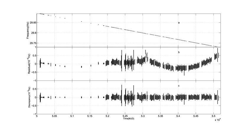
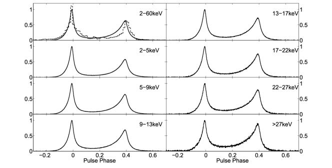
Figure 1: The timing result of the Crab pulsar. Panel $a$ shows the frequency evolution, panel $b$ shows the frequency residuals of the fit with equation(1). and panel $c$ shows the differences between the frequencies measured by X-ray observations and those calculated from the radio ephemeris.

Figure 2: The X-ray profiles of the Crab pulsar in different energy ranges. Phase 0 represents the position of the main radio peak. The dashed line represents the result of the theoretical model (Jia et al., 2007).

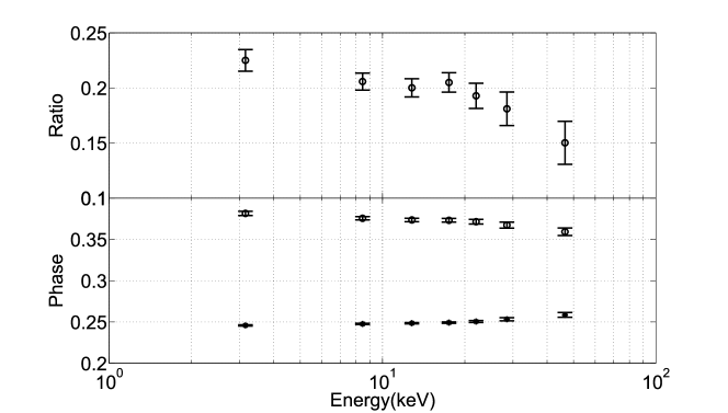
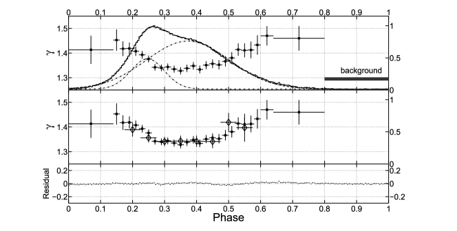
Figure 16: Upper pannel: The intensity fraction of the first narrow Gaussian component of PSR B1509-58 as function of energy. Lower pannel: the positions of the two components in different energy bands. The stars and circle points represent the positions of the narrower and broader components, respectively.

Figure 17: Top pannel: The photon indices of PSR B1509-58 in different phase ranges (“+”). The black belt represents the phase region of the unpulsed background. Middle pannel: Comparison of the photon indices obtained in this work and that by Rots et al. (1998). Bottom pannel: The residuals between the observational profile and the fitted profile.

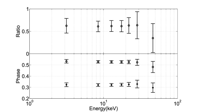
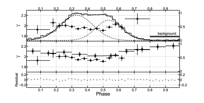
Figure 20: Similar to Fig. 17 but for PSR B0540-69.

Figure 21: Top pannel: The photon indices of PSR B0540-69 in different phase ranges (“+”). The black belt represents the phase region of the unpulsed background. Middle pannel: Comparison of the photon indices obtained in this work and that by (Hirayama et al., 2002). Bottom pannel: The residuals between the observational profile and the fitted profile.

We produce the phase resolved spectra, the response matrixes, and the pulse profiles observation by observation and merge them together according to their respective phase bin for the final profile and spectral analyses. The phase resolved spectra were created by FASEBIN of ftools, and the baseline (unpulsed contribution) was subtracted with FBSUB. The number of phase bin (the NPH parameter for the FASEBIN script, NPH: number of phase bin.) for PSRs B0531+21, B1509-58, and B0540-69 are 200, 50, and 25, respectively and some phase bins will be merged into one bin to guarantee the quality of the spectrum. As there is precise radio ephemerides (including periods and phases) for PSR B0531+21 at ATNF, they were used in the process to produce the phase resolved spectra of this pulsar. For PSRs B1509-58 and B0540-69, since the radio ephemerides are not available for the whole observation duration, the ephemerides derived from the X-ray results were used to gain the phase-resolved spectra, and phase 0 of this observation was obtained by a cross-correlation analysis between its light curve and the reference one. We chose the flat regions of the pulse profiles as the unpulsed background phases (Fig. 2, Fig. 17, and Fig. 21). The unpulsed background phase ranges that correspond to the PHASEMIN and PHASEMAX parameters in FBSUB are 0.63-0.83, 0.8-1.0, and 0.8-1.0 for the three pulsars, as mentioned above. The response matrix for a spectrum was produced with PCARSP. The command to merge the spectrum is ADDSPEC and that to merge the response matrixes is ADDRMF. The weights used in ADDRMF are determined by the total photon counts of the pulse in the corresponding observations. Because PSR B0531+21 is bright, we obtained 42 merged spectra for each phase bin, while for PSR B1509-58 and B0540-69, because they are much fainter, only one merged spectrum has been obtained for each phase bin. The pulse profiles in different energy ranges were gained from the phase-resolved spectra created by the FASEBIN and FBSUB of ftools with more phase bins.

All the spectra were analysed with XSPEC (ver 12.6.0). The spectral model is power law with photoelectric absorption, i.e. [pha*(pl) in XSPEC]. The absorption column density ($N_{H}$) of PSRs B0531+21, B1509-58, and B0540-69 were fixed at 0.36, 1.27, 0.46$\times 10^{22}$ cm^-2 (Massaro et al., 2000; Marsden et al., 1997; Kaaret et al., 2001). For the Crab pulsar, the spectra were also analysed with log-parabola model (Massaro et al., 2000, 2006). The systematic error was set as 0.01. The errors of photon indices are at 90$\%$ confidence level and the errors of the rest data are at 68.3$\%$ confidence level.

3 Results

3.1 Crab

3.1.1 Timing and pulse profiles of the Crab pulsar

To study the timing behaviors of the Crab pulsar we fit its rotation frequencies by a quadratic polynomial (equation (1)). Frequencies and residuals are plotted in Fig. 2a and Fig. 2b respectively, and the fitting results are listed in Table 2. The difference between the X-ray and the radio frequencies are displayed in Fig. 2c The later is from Jodrell Bank Observatory . It is clear that several glitches occurred in this duration, and the X-ray derived frequencies are consistent with the radio ephemerides. Therefore, the radio ephemerides are used when we produce the X-ray pulse profiles in different energy bands and the phase resolved X-ray spectra.

The profiles of the Crab pulsar are created by FASEBIN and FBSSUM of ftools. For each photon event, the RXTE clock corrections and the barycenter corrections based on the JPL DE-200 solar system ephemeris are applied. Then the absolute phase is calculated by referencing to the radio timing ephemeris. Therefore, for an X-ray pulse profile in a specific energy range created by FBSSUM, the phase is the relative phase to the main radio peak. Because a large number of photons have been collected from the Crab pulsar, the period is divided into 1000 phase bins so as to show the detailed structure of the light curve. The energy ranges used to create the light curves are 2-60, 2-5, 5-9, 9-13, 13-17, 17-22, 22-27, and $>$27 keV, corresponding to PCA channels 0-255, 0-10, 11-20, 21-30, 31-40, 41-50, 51-60, and 61-255, respectively. The resulted light curves are plotted in Fig. 2, where phase 0 represents to the position of the main radio peak as mentioned above. Obviously, the shape of the light curve varies with energy.

In order to obtain the phases of the two X-ray peaks more accurately than the size of the phase bin, we fit them with an empirical formula proposed by Nelson et al. (1970).

$$L(\phi-\phi_{0})=N\frac{1+a(\phi-\phi_{0})+b(\phi-\phi_{0})^{2}}{1+c(\phi-\phi_{0})+d(\phi-\phi_{0})^{2}}e^{-f*(\phi-\phi_{0})^{2}}+l,$$ (2)

where $L$ is the intensity at phase $\phi$, $l$ the baseline of the light curve, $\phi_{0}$ the phase shift, $N$ the pulse height of the profile, and $a$, $b$, $c$, $d$ and $f$ the shape coefficients. The pulse phase is measured in phase units, range (0,1). The coefficients of the two peaks were fitted separately, since the width of the main peak broadens with energy increasing (Mineo et al., 1997; Massaro et al., 2006), which is verified in this work and the shapes of the second peak are different from the main peak.

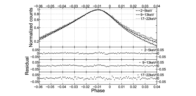
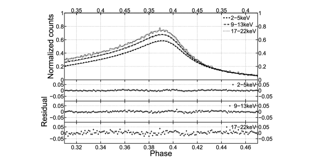
Figure 3: The shape of the main peak of the Crab profile in three energy ranges: 2-5 keV, 9-13 keV, 17-22 keV. Phase 0 represents the position of the main radio peak. The dashed line, dot-dashed line, and dotted line represent the fitted profiles with Nelson’s formula separately in these three energy ranges.

Figure 4: The shape of the second peak of the Crab profile in three energy ranges: 2-5 keV, 9-13 keV,17-22 keV. Phase 0 represents the position of the main radio peak. The dashed line, dot-dashed line, and dotted line represent the fitted profiles with Nelson’s formula separately in these three energy ranges.

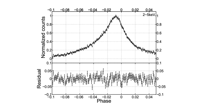
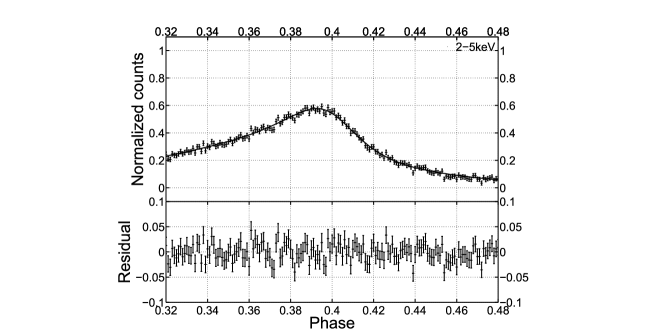
Figure 5: Upper pannel: The fitted profile of the main peak of the Crab profile with fixed parameters of Nelson’s formula for observational ID 60080-01-03-00(profile phase range:-0.29 to 0.07). Lower pannel: The residuals between the observational profile and fitted profile. The reduced $\chi^{2}$ is 0.99 with d.o.f. 358.

Figure 6: Upper pannel: The fitted profile of the second peak of the Crab profile with fixed parameters of Nelson’s formula for observational ID 60080-01-03-00(profile phase range: 0.32 to 0.71). Lower pannel: The residuals between the observational profile and fitted profile. The reduced $\chi^{2}$ is 1.00 with d.o.f. 388.

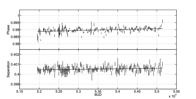
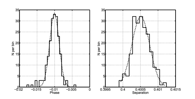
Figure 7: Upper pannel: The phase of the X-ray main peak of the Crab pulsar relative to the radio phase from the Jordell Bank radio ephemeris, in while the phase of the radio main peak is 1.0. Lower pannel: The separation of the two X-ray peaks in different epoches.

Figure 8: Left pannel: The distribution of the phase-lag between the X-ray main peak and the radio main peak of the Crab pulsar with bin size $5.8\times 10^{-4}$ periods. The dashed line represents the fitted Gaussian function with $\mu=-0.0101$ and $\sigma=1.3\times 10^{-3}$. Right pannel: The distribution of the separation between the two X-ray peaks with bin size $9.6\times 10^{-5}$ periods. The dashed line represents the fitted Gaussian function with $\mu=0.4005$ and $\sigma=2.5\times 10^{-4}$.

The fitting procedures of the two peak profiles can be divided into two steps: (1) Obtain the coefficients $a$, $b$, $c$, $d$, $f$ , as well as $N$, $l$, and $\phi_{0}$ from the fitting with the Nelson’s formula to the profiles (Fig. 2) accumulated from all the observations. The fitted profiles of the main peak and the second peak in three energy ranges: 2-5 keV, 9-13 keV, and 17-22 keV are displayed in Fig. 4 and Fig. 4, respectively. The final shape parameters of the two peaks in different energy ranges are listed in Table. 4; (2) Each of the 211 observed profiles in a specific energy range is fitted with the Nelson’s formula coefficients of which are fixed except $N$, $\phi_{0}$, and $l$. The comparisons of one observational profile with the fitted profiles for the two peaks are shown in Fig. 6 and Fig. 6. The reduced $\chi^{2}$ of the main peak and the second peak are 0.99 (d.o.f. 358) and 1.00 (d.o.f. 388), showing that the profiles could be properly fitted. The position of the maximum of the fitted profile is taken as the phase of the main peak, while the separation of the positions of the two maxima is taken as the separation of the two peaks. Fig. 8 plots the 211 phase-lags and separations, in which the errors of the phase-lags are a combination of the main peak phase errors and the rms deviations of the radio timing ephemerides, while the errors of the separations are obtained from the errors of the phases of the two peaks. The phase errors of the X-ray main and second peaks used in the above calculation are obtained from the parameter $\phi_{0}$ in the fitting processes.

Averaging the fitting results to the 211 light curves in 2-60 keV, we found that the phase of the X-ray main peak (2-60 keV) leads the radio main peak with a mean value of 0.0101$\pm$0.0001 periods (Fig. 8) and the mean separation between the main peak and the second peak is 0.40051$\pm$0.00003 periods. Here the error of the phase-lag between the X-ray main peak and the radio main peak is estimated from the distribution of the phase-lag values of the 211 X-ray light curves, and the error of the separation between two X-ray peaks is obtained similarly. As shown in the left panel of Fig. 8, the 211 phase-lags distribute as a Gaussian shape. We then fit the distribution with a Gaussian function, with three free parameters: namely the normalization G, the mean $\mu$, and the standard deviation $\sigma$. $\sigma$ is regarded as the standard deviation of the phase-lag measured from one light-curve, and the standard error of the mean phase-lag is estimated by $\sigma/\sqrt{N}$, where $N=211$, the number of the phase-lags from which the mean is obtained. The fitted mean phase-lag is $\mu=-0.0101$ and $\sigma=1.3\times 10^{-3}$, while the mean phase of the X-ray main peak(2-60 keV) leads the radio main peak by 0.0101$\pm$0.0001 periods. Similarly, as illustrated in the right panel of Fig. 8, the mean separation of the two X-ray peaks is 0.40051$\pm$0.00002 periods. We find that the separations between the two peaks are more concentrated comparing with the phase-lag distribution, implying that the errors of the phase-lags are dominated by the rms deviations of the radio data.

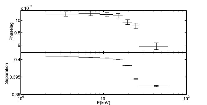
Figure 9: Upper pannel: The phase difference between the X-ray main peak of the Crab pulsar to the radio main peak as a function of X-ray photon energy. Lower Panel: The separation of the two X-ray peaks as a function of energy.

Figure 10: The spectral fit of the Crab pulsar with a absorbed power law ($N_{H}=0.36\times 10^{22}cm^{-2}$) at phase:0.0-0.005. Upper pannel: The crosses represent the observations, and the solid line is the model convolved with the response matrices. Lower pannel: The residuals between the observation data and the best fitted model. The reduced $\chi^{2}$ is 0.99 with the degree of freedom 86.

Previous studies suggested that the phase-lag of the X-ray main peak to the radio main peak and the separation of the two X-ray peaks vary with energy and might change slightly with time (Masnou et al., 1994; Rots et al., 2004; Molkov et al., 2010). We found that the phase lag of the radio peak to the X-ray peak(2-60 keV) shows an increasing trend with time, and a linear fit gives a slope of (6.6$\pm$1.3)$\times$10^-7 periods day^-1. The best fit slope is about two times larger than that obtained by Rots et al. (2004), which is (3.3$\pm$2.0)$\times$10^-7 periods day^-1. However, taking the uncertainty into account, the two measurements are consistent with each other. The separation between the two X-ray peaks does not exhibit such a strong evolutionary trend with time. A linear fit to the data gives a slop of (5.4$\pm$1.8)$\times$10^-8 periods day^-1. The energy dependence of the phase-lag between the radio and X-ray main peaks found by Molkov et al. (2010) is confirmed here (Fig. 10), which reaches the maximum at 5-9 keV and then decreases rapidly. Such an evolutionary trend is consistent with the multi-wavelength behaviors obtained by Kuiper et al. (2003) and Molkov et al. (2010). Fig. 10 also shows that the separation of the two X-ray peaks decreases with the energy, which is consistent with the result of Eikenberry and Fazio (1997). The errors of the phase-lags and separations in different energy ranges are estimated similarly to that in the last paragraph. Affected by the rms deviations of the radio data, the errors of the phase-lags are almost the same with each other as shown in the upper pannel of Fig. 10.

3.1.2 Phase resolved spectral analyses

Since plenty of data were used, we divided the X-ray pulse of the Crab pulsar into 107 sections whose width is determined by the total counts detected in this section, and 42 spectra were created for each section from different observation time intervals. The mean number of counts per bin is 1109.2 and the minimum number of counts per bin is 76.5 after background substraction with energy bins 88. The 42 spectra were fitted with a power-law model and log-parabola (Massaro et al., 2000, 2006) with photoelectric absorption, where the value of N_H was fixed at 0.36$\times$10²²cm^-2 (Massaro et al., 2006). The free parameters of the power law model are the photon index ($\gamma$) and the normalization ($C$):

$$F(E)=CE^{-\gamma}.$$ (3)

While the photon index $\gamma(E)$ in the log-parabola model varies with energy and the normalization is $K$:

$$F(E)=K(E/E_{0})^{-(\alpha+\beta\,Log(E/E_{0}))},$$ (4)

$$\gamma(E)=\alpha+2\beta\,Log(E/E_{0}),$$ (5)

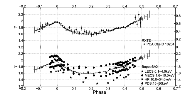
Figure 11: Similar to Fig. 10, but the fitted model is log-parabola with $E_{0}$ fixed at 1 keV. The reduced $\chi^{2}$ is 0.93 with the degree of freedom 85.

Figure 12: Upper pannel: Comparison of the photon indices obtained in this work(“+”) and that by Pravdo et al. (1997). Lower pannel: Comparison of the photon indices obtained in this work and the results observed by the four instruments of BeppoSAX. (Massaro et al., 2000)

where $E_{0}=1$ keV. Both models were used to fit the phase-resolved spectra of the Crab pulsar simultaneously in order to compare the differences between them. The comparisons between the two models fitting the spectrum at phase: 0.0-0.005 are shown in Fig. 10 and Fig. 12. The result shows that power-law model and log-parabola model were both suitable to fit the spectra of the Crab pulsar in the energy range of 3-60 keV. The mean of the 42 $\gamma$ values weighted by photon numbers of the pulse, just as used in ADDRMF, was taken as the final results of the photon index:

$$\gamma_{mean}=\sum w_{i}\gamma_{i}.$$ (6)

$$w_{i}=c_{i}/\sum c_{i},$$ (7)

where $c_{i}$ is the photon number of the pulse and $w_{i}$ is the weight. The error of the mean photon index was obtained from the weighted sample variance. It is the same for $C$ and parameters for log-parabola model. Data points below 3 keV and above 60 keV were ignored for the spectral analyses due to the low signal to noise ratios.

The fitted spectral parameters of the 107 pulse sections with the power law model are listed in Table. 5, and the photon indices are plotted in Fig. 12. It is clear that the spectrum softens from the leading edge of the first peak to the first intensity maximum, hardens through the inter peak and softens again through the second peak. Such an evolutionary trend is consistent with that reported by Pravdo et al. (1997) and Massaro et al. (2000) (Fig. 12). The photon indices of this study are close to the results of HP and between the results of MECS and PDS of BeppoSAX. However, according to the higher accuracy of the present study, more details are revealed: (1) The photon index changes smoothly, without any small bump between the two peaks; (2) The hardest spectrum ($\gamma\sim 1.60$) occurs in phase range 0.12-0.22, in which the intensity also reaches the minimum between the two peaks; (3) The spectrum softens slowly in the rising wing of the second peak and the softening suddenly becomes much rapid from the maximum of the peak. In order to describe the changes of the photon indices, the pulse phase was divided into ten intervals and the relations of photon indices with phase were fitted with a linear function in each interval. The results are listed in Table. 7. The absolute slope values are different on both sides of the main peak, which means the change is asymmetric. For the second peak, the slope value of the tailing side is obviously larger than that of the leading edge just as the previous description. To integrate all the 107 spectra, the total absorbed flux of Crab’s pulse is (1.996$\pm$0.001)$\times$10^-9 ergs s^-1 cm^-2 in the 2-10 keV band.

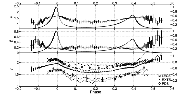
Figure 13: The results of the phase-resolved spectra of the Crab pulsar with log-parabola model in different phase ranges. Upper pannel: The parameter $\alpha$ in the log-parabola model. Middle pannel: The parameter $\beta$ in the log-parabola model. Bottom pannel: The comparison of the photon indices of the power law model and spectral indices calculated from equation 5 where $E=1.5,9.3,30.0\,keV$. The solid line represents the energy dependent photon indices for RXTE. The two dot-dashed lines represent $1\sigma$-uncertainties from the extrapolation of the spectral distribution for LECS of BeppoSAX. The dashed lines are similar to dot-dashed lines but for PDS of BeppoSAX. The square, “+”, and diamond points represent the results of LECS, PCA, and PDS respectively.

The results of the phase-resolved spectra with log-parabola model are listed in Table. 8, and parameters $\alpha$ and $\beta$ of the model in different phase ranges are plotted in Fig. 13. The evolution of parameter $\alpha$ is similar to the evolution of the photon index of the power law model except in the trailing wing of the second peak. In the trailing wing of the second peak, $\alpha$ becomes smaller with phase gradually while the photon indices of the power law increase suddenly. $\beta$ is lower at the two peaks, $\thicksim$0.16, moderate at the interpeak region, $\thicksim$0.2, and higher in the leading edge of the first peak(phase -0.14- -0.05) and the trailing edge of the second peak(phase 0.45-0.55), $\thicksim$0.4. The positive value of the $\beta$ means that the photon indices in all phase ranges increase with energy and larger $\beta$ means that the spectra softens faster than in the other phase ranges. The result is consistent with the conclusion of Massaro et al. (2000) and Massaro et al. (2006) (Fig. 12). The energy dependent photon indices can be calculated from equation 5 and its evolution is similar to the evolution of the photon indices of the power law model as shown in Fig. 13 at $E=9.3$ keV.

Using Ftest, we find that the log-parabola model is more suitable than the power law model as to describing the X-ray spectrum in each phase bin. As shown in Table. 8, the substitution of the power law model by the log-parabolic model is necessary at a significance level of $>99.9\%$ in the two peak regions (phase -0.03- 0.01 and phase 0.365-0.405). We also check whether the extrapolation of the parabolic spectral model is consistent with the observations in the adjacent energy ranges, such as the results of LECS and PDS of BeppoSAX. As shown in Fig. 13, the results of the extrapolation are consistent with the spectral evolution obtained from LECS and PDS of BeppoSAX (Massaro et al., 2000). To summarize, the log-parabola model is suitable and better than the power law model for the description of the X-ray spectra of the Crab pulsar.

3.2 PSR B1509-58

3.2.1 Timing and Pulse profiles

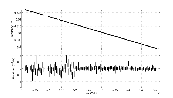
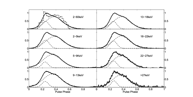
Figure 14: The rotation frequencies of PSR B1509-58 obtained from the X-ray observations (upper pannel) and the residuals of the fit with equation(1) (lower pannel).

Figure 15: The X-ray profiles of PSR B1509-58 in different energy ranges. The two dot-dashed lines represent the two Gaussian components used to fit the pulses. The dashed line represents model result Zhang & Cheng (2000)

For PSR B1509-58 the timing results are showed in Fig. 15. The timing properties of PSR B1509-58 are derived in a similar way to that of the Crab pulsar and the detailed X-ray ephemeris of PSR B1509-58 is listed in Table. 2.

We created the light curves of PSR B1509-58 in the same energy bands as for the Crab pulsar, while the period of PSR B1509-58 was divided into 100 or 200 phase bins due to its much lower flux. The X-ray pulse profile of PSR B1509-58 is broad and asymmetric, with a steep rise and flat decay, and no evolution with energy could be found by eye-balls. Kuiper et al. (1999) and Cusumano et al. (2001) found that its X-ray pulse could be well fitted by two Gaussian functions:

$$L=N_{1}e^{-0.5*(\frac{\phi-\mu_{1}}{\sigma_{1}})^{2}}+N_{2}e^{-0.5*(\frac{\phi-\mu_{2}}{\sigma_{2}})^{2}}+l,$$ (8)

where $N_{1}$, $\mu_{1}$, $\sigma_{1}$, $N_{2}$, $\mu_{2}$, $\sigma_{2}$, and $l$ are free parameters. We therefore fitted the X-ray pulses of PSR B1509-58 in different energy bands with two Gaussian functions so as to quantify the dependency of the X-ray pulse on photon energy. The coefficients and the reduced $\chi^{2}$ are listed in Table. 10. Fitting the 2-60 keV profile derives a narrow component peaking at 0.249$\pm$0.001 with a width of 0.053$\pm$0.001 and a broader component peaking at 0.375$\pm$0.002 with a width of 0.129$\pm$0.002, which are consistent with those obtained by (Kawai et al., 1991), Rots et al. (1998), and Cusumano et al. (2001). The central phases of the two components are slightly different from the results of Kuiper et al. (1999) and Cusumano et al. (2001), which may be caused by discrepant energy bands of the profiles. Fig. 15 displays the pulse profiles in different energy bands fitted with two Gaussian functions, and Fig. 17 plots the relative intensity of the components as well as their central phases. It could be seen that, with the increasing photon energy, the second component becomes stronger and the separation between the two components decreases, implying that the X-ray pulse of PSR B1509-58 is narrower at higher energy.

3.2.2 Phase resolved spectral analyses

We fitted the X-ray spectrum of the 26 phase bins of PSR B1509-58 by a single power law with photoelectric absorption in the energy range 3-30 keV, and the fitting results are listed in Table. 11 and plotted in Fig. 17. In contrast to the results of Rots et al. (1998), who suggested that the spectrum does not change with phase, our results show that the photon index do changes within the pulse. The photon index decreases from 1.4 at the rising edge of the pulse gradually to about 1.32 just at the maximum phase, then keeps constant, and starts to rise at the shoulder of the pulse to about 1.45 at the trailing wing. Comparing our result to that of Rots et al. (1998) (Fig. 17, lower panel) shows that these two results are actually consistent within the error bars, and what makes the difference is that we have used ten times more data than Rots et al. (1998) and so get much smaller error bars. If the photon indices in different phases have the uniform distribution, the $\chi^{2}$ of 26 data points is 335.4, which means photon indices have high significant evolution with phase. The total absorbed flux of the pulse is $(2.30\pm 0.02)\times$10^-11 ergs s ^-1 cm^-2 in the 2-10 keV band, which is consistent with 2.0$\times$10^-11 ergs s ^-1 cm^-2 given by Cusumano et al. (2001).

3.3 PSR B0540-69

3.3.1 Timing and Pulse profiles

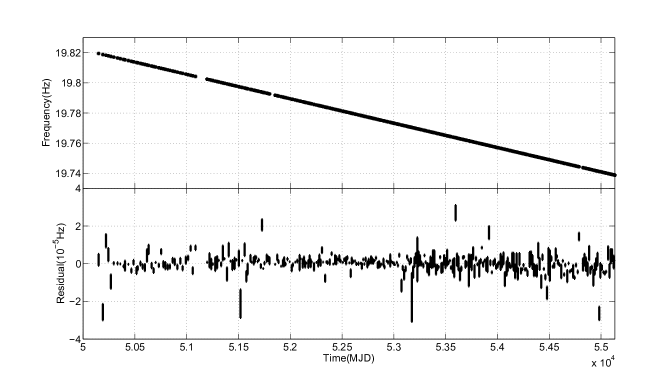
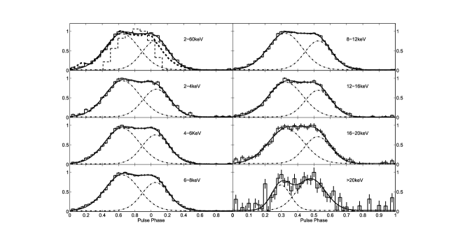
Figure 18: Similar to Fig. 15 but for PSR B0540-69.

Figure 19: The X-ray profiles of PSR B0540-69 in different energy ranges. The two dot-dashed lines represent the two Gaussian components used to fit the pulses. The thin and thick dashed lines represent the model results from Zhang & Cheng (2000) and Takata & Chang (2007) separately.

For PSR B0540-69, the timing results are showed in Fig. 19. The timing properties of PSR B0540-69 are derived in a similar way to that of the Crab pulsar and the detailed X-ray ephemeris of PSR B0540-69 is listed in Table. 2.

Because PSR B0540-69 is the dimmest among the three pulsars, its light curves were created in 2-60, 2-4, 4-6, 6-8, 8-12, 12-16, 16-20, and $>$20 keV bands, correspond to PCA channels 0-255, 0-9, 10-13, 14-18, 19-27, 28-36, 37-47, and 48-255, and one period was divided into 50 phase bins. PSR B0540-69 has a single broad X-ray pulse slightly hollowed in the center (Plaa et al., 2003). The pulse profiles with different energy ranges have no significant variation as from Fig. 19, which is consistent with that given by Plaa et al. (2003) and Campana et al. (2008). The pulse profiles can also be fitted well with two Gaussian functions(Equation 8 and Table. 12). The central phases of the two functions, except the profile above 20 keV that has large uncertainty, are located at about phase 0.32 and 0.53, and their widths are about 0.11 and 0.08 respectively. The separations between two functions in different energy ranges are about 0.21 in phase (Fig. 19). These results are similar to Plaa et al. (2003). The fraction of the first broader pulse accounting for the whole pulse and the central phases of the two Gaussian functions are calculated in a similar way to that for PSR B1509-58. The fraction and the central phases of the two components do not show significant evolution with energy (Fig. 21).

3.3.2 Phase resolved spectral analyses

Totally we created 14 phase resolved spectra of PSR B0540-69 and fitted them in 3-30 keV by a simple power law model with photoelectric absorption. The spectral evolution with phase of PSR B0540-69 is different from the Crab pulsar but similar to PSR B1509-58 (Table. 13 and Fig. 21). The photon indices in the middle of the pulse (phase range 0.3-0.5) is about 1.93 but that for the two wings is about 2.0. The $\chi^{2}$ of 14 data points is 59.8, implying photon indices of PSR B0540-69 have high significant evolution with phase. Such a spectral hardening in the center of the pulse was also obtained by Hirayama et al. (2002) using the 1-10 keV data from the ASCA satellite, though the later suggested a slightly higher photon index in the central region of the pulse. The photon index of the whole pulse is 1.92$\pm$0.02. This agrees with the results by Mineo et al. (1999) (1.94$\pm$0.03) and by Kaaret et al. (2001) (1.92$\pm$0.03). The total absorbed flux of the pulse is (6.4$\pm$0.2)$\times$10^-12 ergs s^-1 cm^-2, which is consistent with 6.5$\times$10^-12 ergs$\cdot$s${}^{-1}\cdot$cm^-2 (Campana et al., 2008) in the 2-10 keV band.

3.4 Photon Index Evolution with Time

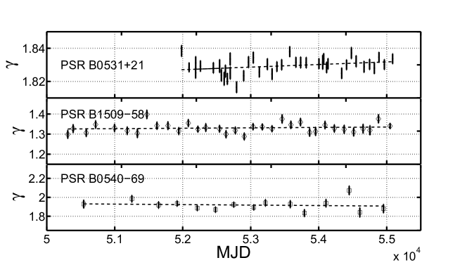
Figure 22: The photon indices of PSRs B0531+21, B1509-58, and B0540-69 in different time.

The long time span of the observations also allows us to study the real time evolution of the spectra of these three pulsars. Plotting the photon indices of the whole pulse at different epochs of the three pulsars suggests that there may exist a slight spectral softening for the Crab pulsar, while PSR B1509-58 and the spectrum of PSR B0540-69 remains unchanged (Fig. 22). We note here that the photon indices of the overall pulsed emission of the Crab pulsar in an epoch is the mean of the 107 phase resolved photon indices weighted by the their errors, while those for PSR B1509-58 and B0540-69 are obtained from the fitting to their whole pulses, respectively. A linear fit to the Crab data gives a slope of (1.6$\pm 0.7)\times 10^{-6}$ day^-1, that for PSR B1509-59 is (2.0$\pm 3.6)\times 10^{-6}$day^-1, and (-5$\pm 14)\times 10^{-6}$day^-1 for PSR B0540-69. Statistically only the Crab pulsar has a significant spectral softening. We note that Hirayama et al. (2002) detected no spectral variation of PSR B0540-69 either.

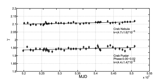
Figure 23: The photon indices of the Crab pulsar and the Crab Nebula. The black lines are the linear fits to the data and $k$ is the value of the slope.

However, the Crab nebula including the pulsar is the calibration source of RXTE. The spectral softening is probably a consequence of the improper calibration. In order to check whether the spectral evolution results we obtained above is reliable or not, we first studied such spectral evolution for different phase ranges, which is carried out under the consideration that the improper calibration would make the spectra in different phase-bins to have the similar softening slope. We find that all the slopes are higher than zero, and there do exists a structure in the phase range of the main peak, i.e., the spectral softening is more significant in the two wings. However, the $\chi^{2}$ is 24.4(18 d.o.f), showing that the spectral variety in each phase has the similar softening slope. On another hand, the spectra of the Crab Nebula were also analysed with the absorbed power law model and were extracted from the Standard 2 data of PCU2 with all layers in epoch 5 of RXTE. The spectral indices were fitted with a linear function and the slope is $(4.7\pm 1.6)\times 10^{-6}day^{-1}$, which is comparable to the mean slope of all phases: $(5.3\pm 0.5)\times 10^{-6}day^{-1}$ (Fig. 23). For the rest PCUs, the results are similarly with Jahoda et al. (2006) and Weisskopf et al. (2010). The spectrum in every phase softening with time may be caused by the tiny deviation of the calibration.

4 Discussion

4.1 Comparison of the pulse profiles with model predictions

The X-ray pulse of the Crab pulsar is composed of two peaks and inter peak region and changes significantly with energy. Jia et al. (2007) have calculated the light curves of the Crab pulsar with assumption that inner boundary is extended inward from the null charge surface to 10 stellar radii(Fig. 2). The X-ray profile of the Crab pulsar predicted by their model is consistent with the observational data except the second peak with inclination angle 50^º and viewing angle 75^º. The intensity of the leading edge of the second peak is evidently smaller than the observational profile. Tang et al. (2008) gave a profile in Fig. 5 of their paper. However, that profile is obviously different from our results. Specifically, the intensity of the second peak in their paper is higher than that of the first peak, while in our observation the first peak has significantly higher intensity. The profile predicted by Harding et al. (2008) has at least 4 peaks, which has not be detected in our high statistical results, and thus their model is unsuitable. Du et al. (2010) only give the high energy pulse profiles of the Crab pulsar($>$0.1GeV), while our observation is in the energy range lower than 60 keV.

The X-ray pulses of PSRs B1509-58 and B0540-69 are broad asymmetric profiles showing no obvious change with energy, which are different from the Crab pulsar. The X-ray pulses of PSRs B1509-58 and B0540-69 can be fitted with two Gaussian curves(Kuiper et al., 1999; Cusumano et al., 2001; Plaa et al., 2003). Zhang & Cheng (2000) have calculated the light curves of PSRs B1509-58, and B0540-69 (Fig. 15, and Fig. 19). For PSR B1509-58, the predicted profile is sharp at edges and the top of profile has two peaks comparing with the observed profile with inclination angle 60^º and viewing angle 75^º. For PSR B0540-69, the predicted profile is narrower than the observed profile with inclination angle 50^º and viewing angle 76^º. Takata & Chang (2007) recalculate the profile of PSR B0540-69 (Fig. 19) with inclination angle 30^º and viewing angle 81.5^º. The profile of PSR B0540-69 predicted by their model are consistent with the observational results. The small peak located at the leading edge of the pulse is larger while the trailing edge of pulse is smaller than the observation profile. However, these models give surprising results to interpret the observations, more specifics need to be considered in detailed modeling.

4.2 Constrains from the phase-resolved spectra

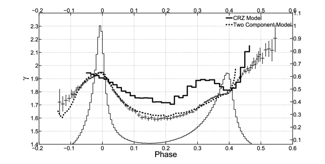
Figure 24: The photon indices of the Crab pulsar in different phase ranges (“+”). The thick solid line represents the model prediction by the CRZ model (Zhang and Cheng, 2002) and the dashed line represents the two-component model(Massaro et al., 2000).

We confirmed the variation of Crab’s spectrum with phase as detected in the previous studies, and found a rapid softening in the trailing edge of the second peak. Pravdo et al. (1997) and Massaro et al. (2000) have given the similar results, which are plotted in Fig. 12. Comparing to their result, we have obtained more spectral indices, including the leading edge of the first peak and the trailing edge of the second peak. Our results show that the photon index variation between the two peaks is very smooth, without any small bump that can not be excluded by the previous low statistic analyses (e.g., Pravdo et al. 1997 and Massaro et al. 2000). We find that hardest spectrum occurs positionally coincide with the minimum intensity in the inter peak region, which is unclear in the analyses of Pravdo et al. (1997). Those new results set stronger constraints on the theoretical models of pulsar high energy emission. Zhang and Cheng (2002) calculated the phase resolved X-ray spectrum of the Crab pulsar using the CRZ model with only the synchrotron radiation from the secondary pairs being considered. Their calculation can explain the rapid spectral softening of the trailing edge of the second peak (Fig. 24). However, from the comparison we know that their model prediction is different from observations in the following aspects: (1) the observed spectrum in the leading edge of the first peak softens when approaching the intensity maximum and then hardens, while the model prediction is that the spectrum hardens all through the first peak; (2) the spectrum of the inter-peak region is significantly and systematically harder than the model prediction; and (3) the model predicts ahead of the second peak a softer region that can be excluded by observations. These discrepancies will set tight constrains on the future pulsar X-ray emission models and their parameters.

The phase resolved spectra of PSR B1509-58 are calculated here in narrower and more phase bins compared to the work of Rots et al. (1998) (diamond points in Fig. 17). They vary with phase and do not follow the intensity of the profile. The photon indices are about 1.33$\pm$0.01 in the center part of the pulse (0.25-0.5) and become softer in the wings. Such a spectral evolution is apparently different from the behaviors of the two peaks of the Crab pulsar. However, if the pulse profile of PSR B1509-58 is a combination of two Gaussian components as pointed out by Kuiper et al. (1999) and Cusumano et al. (2001), the hardest spectrum will be between the two components (Fig. 15 and Fig. 17), which is similar to that of the Crab pulsar. The phase resolved spectra of PSR B0540-69 are similar to PSR B1509-58, albeit with lower statistics and thus larger uncertainties. The broad pulse of PSR B0540-69 can be de-composed into two narrower Gaussian pulses too (Plaa et al., 2003). Thus its overall spectral evolutionary trend is also similar to that of the Crab pulsar, as shown in Fig. 21. Massaro et al. (2000) proposed that the pulsed emission of the Crab pulsar can be described as the superposition of optical component($C_{O}$) and X-ray component($C_{X}$). The phase-resolved spectra of the Crab pulsar in the two-component model can also be calculated from the ratio of the summed intensities of $C_{O}$ and $C_{X}$ at two extreme values:

$$\gamma_{12}=\frac{Log(F(E_{2})/F(E_{1}))}{Log(E_{2}/E_{1})}+\gamma_{O},$$ (9)

where $E_{1}=3$ keV, $E_{2}=60$ keV, and $\gamma_{O}=1.95$. As shown in Fig. 24, the results agree with the spectral evolution of the Crab pulsar except at the tail edge of the second peak, where the model predicted photon indices are smaller than the observed ones.

5 Summary

It is shown with the RXTE data that the spectra of PSRs B0531+21, B1509-58 and B0540-69 all evolve with pulse phase. In addition to the previous results of PSR B0531+21, which has been confirmed with a much higher statistics, we found that the spectral softening increases immediately after the second peak. Our analyses show that the spectra of PSR B1509-58 and B0540-69 are harder at the centers of the pulses and are softer at the wings, which are different from that of the Crab pulsar, whose spectrum is softer at the two peaks. However, since the pulses of PSRs B1509-58 and B0540-69 could be further decomposed each into two narrower Gaussian components, their overall spectral evolution with phase is thus similar to the Crab pulsar. These new results set more constraints on pulsar X-ray emission models.

Table 1: The parameters of PSRs B0531+21, B1509-58 & B0540-69

Pulsar Name	P	$\dot{P}$	$\tau$	$B$	$E_{rot}$	$L_{X}$	$\gamma$	Braking Index
	(ms)	$(10^{-15}\,ss^{-1})$	(yr)	$(10^{12}G)$	$(10^{38}\,ergs^{-1})$	$(10^{36}\,ergs^{-1})$
Crab	33	423	1240	1.2	4.7	1.3a	2.022(14)1	2.509(1)8
PSR B1509-58	150	1540	1560	4.8	0.18	0.47b	1.358(14)2	2.837(1)9
								2.80(3)10
PSR B0540-69	50	480	1670	1.6	1.5	4.0a	2.1(2)3	1.81(7)11
							1.845(4)4	2.125(1))12
							1.83(13)5	2.140(9)13
							1.94(3)6
							1.3(5)7

Note: 1) 1: Kuiper et al. (2001), 2: Marsden et al. (1997), 3: Campana et al. (2008), 4: Plaa et al. (2003), 5: Kaaret et al. (2001), 6: Mineo et al. (1999), 7: Finley (1993), 8: Lyne et al. (1988), 9: Kaspi et al. (1994), 10: S. Johnston & D. Galloway (1999), 10: Zhang et al. (2001), 12: Cusumano et al. (2003), 13: Livingstone et al. (2005)

2) a: energy range: 2-10 keV (Kaaret et al. (2001)) b: energy range: 2-250 keV (Marsden et al. (1997))

Table 2: The timing results of PSRs B0531+21, B1509-58, and B0540-69 from the X-ray Observations

	PSR B0531+21	PSR B1509-58	PSR B0540-69
R.A.	$05^{h}34^{m}31^{s}.972$	$15^{h}13^{m}55^{s}.620$	$05^{h}40^{m}11^{s}.202$
Decl.	22º00′52′′.07	-59º08′9′′.00	-69º19′54′′.17
Epoch(MJD)	52247.0	52656.0	52656.0
F0(Hz)	29.82341787(28)	6.61254815(23)	19.7787959(11)
$\dot{F}$(10-10s-2)	-3.740484(16)	-0.669734(13)	-1.873520(65)
$\ddot{F}$(10-21s${}^{-3})$	9.545(24)	1.933(22)	3.73(11)
Braking index	2.035(5)	2.85(3)	2.10(6)

Table 3: The list of RXTE observations used in this work

Pulsar	Obs ID	Start Date	End Date	offset(’)	exposure(s)
	50099	2001-02-15	2001-08-27	0.03	7504
	60079	2001-09-10	2002-10-22	0.03	20240
	60080	2001-07-18	2001-07-20	0.03	3776
	60420	2001-09-07	2001-09-09	0.03	1824
	70018	2002-05-09	2003-05-14	0.03	9616
Crab	70802	2002-11-07	2003-02-26	0.03	7888
	80802	2003-03-13	2004-02-15	0.03	17552
	90802	2004-02-29	2005-02-25	0.03	18032
	91802	2005-03-13	2006-02-10	0.03	17088
	92802	2006-03-11	2006-09-24	0.03	23536
	93802	2007-07-17	2008-12-17	0.03	28768
	94802	2008-12-31	2009-11-07	0.03	16768
	total exposure(s)				172592
	10208	1996-03-06	1996-10-16	0.01	14640
	20802	1996-11-15	1997-12-21	0.01	39056
	30704	1998-07-15	1999-01-13	0.01	17984
	40704	1999-02-10	2000-03-16	0.01	43920
	50705	2000-04-20	2001-03-29	0.01	39408
PSR B1509-58	60703	2001-04-28	2002-03-28	0.01	53520
	70701	2002-04-25	2003-04-04	0.01	51056
	80803	2003-05-22	2004-02-26	0.01	45408
	90803	2004-03-25	2005-02-18	0.01	52080
	91803	2005-03-21	2006-02-23	0.01	48464
	92803	2006-03-22	2007-06-22	0.01	75744
	93803	2007-07-12	2008-12-19	0.01	80256
	94803	2009-01-20	2009-10-26	0.01	44160
	total exposure(s)				578288
	10206	1996-08-11	1996-11-17	0.01	11088
	10218	1996-10-12	1996-12-22	21.7	31552
	10250	1996-10-04	1996-03-08	24.9	14016
	20188	1996-12-30	1997-12-12	24.8	51744
	30087	1998-01-04	1998-09-30	24.8	40624
	40139	1999-01-19	2000-02-15	16.1	187392
	50103	2001-03-15	2001-03-05	15.9	246880
	50414	2000-06-05	2000-06-23	5.3	7040
PSR B0540-69	60082	2001-03-26	2003-02-21	15.8	265936
	70092	2002-03-21	2003-04-04	15.9	292032
	80089	2003-04-16	2004-10-29	15.9	339904
	80118	2004-01-07	2004-01-09	24.4	48064
	90075	2004-03-10	2005-05-09	16.0	188256
	91060	2005-05-24	2006-05-14	15.9	216496
	92010	2006-03-12	2007-06-22	15.9	250976
	93023	2007-07-02	2007-06-30	15.9	304192
	93448	2008-09-09	2008-11-17	15.9	39296
	94023	2008-12-26	2009-10-28	15.9	165392
	total exposure(s)				2662528

Table 4: The coefficients of the Nelson’s formula for the main peak and the second peak of the Crab pulsar

	Energy range(keV)	a	b	c	d	e	$\chi^{2}_{dof}$	d.o.f.
	2-60	-12.33193	1078.13826	15.05149	3870.43735	195.75749	2.8	342
	2-5	-13.76710	1001.72137	6.87700	3843.36216	203.31147	2.0	342
	5-9	-11.79666	1100.25133	16.59565	3858.08309	191.78127	1.8	342
Main peak	9-13	-7.75976	1069.76546	27.38679	3535.79500	177.79887	1.6	342
	13-17	-5.96624	1205.02963	33.87094	3629.01368	173.93670	1.4	342
	17-22	-3.54120	1102.97976	35.51093	3210.66333	167.27991	1.4	342
	22-27	-0.18720	1202.12570	42.07548	3268.22696	160.77189	1.4	342
	27-60	0.86096	1527.74475	33.16336	4033.16928	174.22816	1.1	342
	2-60	-23.85914	259.29529	-37.77808	516.20914	97.90285	2.9	443
	2-5	-23.97517	280.84606	-38.68251	577.13359	98.38800	1.8	443
	5-9	-23.76023	251.13817	-37.33119	495.12274	97.12726	2.0	443
Second peak	9-13	-23.77675	231.10693	-36.28714	441.03471	90.70316	1.7	443
	13-17	-23.08951	212.20550	-35.21583	406.45133	92.79225	1.3	443
	17-22	-18.24024	122.91978	-28.28962	237.51385	69.65176	1.5	443
	22-27	-17.27004	105.47879	-26.53128	203.78858	62.65549	1.4	443
	27-60	-17.32346	102.82002	-25.53566	184.54082	63.96669	1.1	443

Table 5: The phase-resolved spectral analysis results of the Crab pulsar for power law model

Pulse phase range	Normalization	Spectral Index	$\chi^{2}$	d.o.f.
-0.140…-0.130	0.045 $\pm$ 0.006	1.721 $\pm$ 0.098	95.4	86
-0.130…-0.120	0.060 $\pm$ 0.005	1.708 $\pm$ 0.055	91.4	86
-0.120…-0.110	0.098 $\pm$ 0.007	1.735 $\pm$ 0.039	92.3	86
-0.110…-0.100	0.147 $\pm$ 0.007	1.750 $\pm$ 0.025	91.3	86
-0.100…-0.095	0.195 $\pm$ 0.011	1.784 $\pm$ 0.031	91.4	86
-0.095…-0.090	0.226 $\pm$ 0.011	1.777 $\pm$ 0.026	89.3	86
-0.090…-0.085	0.276 $\pm$ 0.012	1.784 $\pm$ 0.022	89.7	86
-0.085…-0.080	0.346 $\pm$ 0.013	1.813 $\pm$ 0.020	93.7	86
-0.080…-0.075	0.421 $\pm$ 0.013	1.830 $\pm$ 0.016	94.8	86
-0.075…-0.070	0.495 $\pm$ 0.014	1.829 $\pm$ 0.014	93.5	86
-0.070…-0.065	0.585 $\pm$ 0.014	1.836 $\pm$ 0.012	94.9	86
-0.065…-0.060	0.711 $\pm$ 0.016	1.856 $\pm$ 0.011	90.7	86
-0.060…-0.055	0.854 $\pm$ 0.019	1.870 $\pm$ 0.010	93.1	86
-0.055…-0.050	1.007 $\pm$ 0.018	1.876 $\pm$ 0.008	93.6	86
-0.050…-0.045	1.202 $\pm$ 0.021	1.888 $\pm$ 0.007	97.4	86
-0.045…-0.040	1.427 $\pm$ 0.022	1.900 $\pm$ 0.006	96.6	86
-0.040…-0.035	1.672 $\pm$ 0.024	1.903 $\pm$ 0.005	99.3	86
-0.035…-0.030	1.985 $\pm$ 0.027	1.910 $\pm$ 0.005	101.7	86
-0.030…-0.025	2.343 $\pm$ 0.028	1.914 $\pm$ 0.004	100.2	86
-0.025…-0.020	2.801 $\pm$ 0.032	1.921 $\pm$ 0.004	103.5	86
-0.020…-0.015	3.407 $\pm$ 0.039	1.933 $\pm$ 0.003	109.8	86
-0.015…-0.010	4.114 $\pm$ 0.045	1.941 $\pm$ 0.003	115.3	86
-0.010…-0.005	4.900 $\pm$ 0.049	1.948 $\pm$ 0.003	120.5	86
-0.005…-0.000	5.382 $\pm$ 0.049	1.949 $\pm$ 0.002	119.8	86
-0.000…0.005	5.108 $\pm$ 0.042	1.947 $\pm$ 0.003	120.5	86
0.005…0.010	4.047 $\pm$ 0.044	1.933 $\pm$ 0.003	109.6	86
0.010…0.015	2.958 $\pm$ 0.038	1.909 $\pm$ 0.004	103.2	86
0.015…0.020	2.189 $\pm$ 0.032	1.882 $\pm$ 0.005	100.2	86
0.020…0.025	1.693 $\pm$ 0.022	1.862 $\pm$ 0.005	97.4	86
0.025…0.030	1.353 $\pm$ 0.019	1.844 $\pm$ 0.006	91.0	86
0.030…0.035	1.081 $\pm$ 0.018	1.814 $\pm$ 0.007	92.0	86
0.035…0.040	0.904 $\pm$ 0.016	1.800 $\pm$ 0.008	99.2	86
0.040…0.045	0.772 $\pm$ 0.015	1.786 $\pm$ 0.009	92.9	86
0.045…0.050	0.667 $\pm$ 0.014	1.768 $\pm$ 0.009	94.3	86
0.050…0.055	0.592 $\pm$ 0.013	1.760 $\pm$ 0.011	90.4	86
0.055…0.060	0.519 $\pm$ 0.012	1.739 $\pm$ 0.012	93.2	86
0.060…0.065	0.471 $\pm$ 0.012	1.728 $\pm$ 0.012	94.4	86
0.065…0.070	0.423 $\pm$ 0.011	1.718 $\pm$ 0.013	92.6	86
0.070…0.075	0.382 $\pm$ 0.011	1.699 $\pm$ 0.013	95.7	86
0.075…0.080	0.355 $\pm$ 0.010	1.694 $\pm$ 0.014	92.4	86
0.080…0.090	0.305 $\pm$ 0.008	1.670 $\pm$ 0.011	92.6	86
0.090…0.100	0.274 $\pm$ 0.008	1.661 $\pm$ 0.012	95.8	86
0.100…0.110	0.250 $\pm$ 0.007	1.649 $\pm$ 0.013	92.5	86
0.110…0.120	0.227 $\pm$ 0.007	1.623 $\pm$ 0.013	89.7	86
0.120…0.130	0.208 $\pm$ 0.006	1.604 $\pm$ 0.013	92.9	86
0.130…0.140	0.205 $\pm$ 0.006	1.608 $\pm$ 0.015	91.7	86
0.140…0.150	0.198 $\pm$ 0.006	1.595 $\pm$ 0.014	93.6	86
0.150…0.160	0.201 $\pm$ 0.006	1.602 $\pm$ 0.014	90.3	86
0.160…0.170	0.197 $\pm$ 0.006	1.592 $\pm$ 0.014	90.4	86
0.170…0.180	0.203 $\pm$ 0.006	1.592 $\pm$ 0.014	90.1	86
0.180…0.190	0.212 $\pm$ 0.006	1.597 $\pm$ 0.013	89.6	86
0.190…0.200	0.223 $\pm$ 0.006	1.601 $\pm$ 0.013	93.1	86
0.200…0.210	0.232 $\pm$ 0.006	1.596 $\pm$ 0.012	91.7	86
0.210…0.220	0.247 $\pm$ 0.006	1.597 $\pm$ 0.011	93.5	86
0.220…0.230	0.270 $\pm$ 0.006	1.607 $\pm$ 0.011	95.3	86
0.230…0.240	0.297 $\pm$ 0.007	1.611 $\pm$ 0.009	93.1	86

Table 6: The phase-resolved spectral analysis results of the Crab pulsar for power law model-continued

Pulse phase range	Normalization	Spectral Index	$\chi^{2}$	d.o.f.
0.240…0.250	0.321 $\pm$ 0.007	1.617 $\pm$ 0.009	91.0	86
0.250…0.260	0.355 $\pm$ 0.007	1.623 $\pm$ 0.009	97.2	86
0.260…0.270	0.396 $\pm$ 0.007	1.632 $\pm$ 0.008	93.8	86
0.270…0.280	0.447 $\pm$ 0.008	1.643 $\pm$ 0.007	95.9	86
0.280…0.290	0.496 $\pm$ 0.008	1.647 $\pm$ 0.007	96.1	86
0.290…0.300	0.571 $\pm$ 0.009	1.662 $\pm$ 0.006	97.4	86
0.300…0.305	0.664 $\pm$ 0.011	1.682 $\pm$ 0.008	95.3	86
0.305…0.310	0.730 $\pm$ 0.013	1.698 $\pm$ 0.007	97.8	86
0.310…0.315	0.765 $\pm$ 0.012	1.696 $\pm$ 0.007	93.7	86
0.315…0.320	0.826 $\pm$ 0.013	1.704 $\pm$ 0.006	96.7	86
0.320…0.325	0.905 $\pm$ 0.013	1.720 $\pm$ 0.006	97.2	86
0.325…0.330	0.973 $\pm$ 0.014	1.725 $\pm$ 0.006	94.4	86
0.330…0.335	1.046 $\pm$ 0.015	1.732 $\pm$ 0.006	99.1	86
0.335…0.340	1.131 $\pm$ 0.015	1.739 $\pm$ 0.005	99.1	86
0.340…0.345	1.225 $\pm$ 0.016	1.749 $\pm$ 0.005	101.0	86
0.345…0.350	1.318 $\pm$ 0.017	1.752 $\pm$ 0.005	101.9	86
0.350…0.355	1.422 $\pm$ 0.019	1.759 $\pm$ 0.005	99.8	86
0.355…0.360	1.548 $\pm$ 0.017	1.766 $\pm$ 0.004	101.8	86
0.360…0.365	1.671 $\pm$ 0.020	1.768 $\pm$ 0.004	98.0	86
0.365…0.370	1.812 $\pm$ 0.021	1.776 $\pm$ 0.004	103.7	86
0.370…0.375	1.962 $\pm$ 0.021	1.779 $\pm$ 0.003	103.2	86
0.375…0.380	2.102 $\pm$ 0.022	1.779 $\pm$ 0.004	102.2	86
0.380…0.385	2.265 $\pm$ 0.024	1.783 $\pm$ 0.003	100.6	86
0.385…0.390	2.397 $\pm$ 0.024	1.784 $\pm$ 0.003	102.7	86
0.390…0.395	2.465 $\pm$ 0.024	1.784 $\pm$ 0.003	103.7	86
0.395…0.400	2.471 $\pm$ 0.024	1.789 $\pm$ 0.003	103.9	86
0.400…0.405	2.344 $\pm$ 0.023	1.800 $\pm$ 0.003	106.7	86
0.405…0.410	2.067 $\pm$ 0.022	1.812 $\pm$ 0.004	97.7	86
0.410…0.415	1.778 $\pm$ 0.020	1.832 $\pm$ 0.004	98.1	86
0.415…0.420	1.528 $\pm$ 0.021	1.857 $\pm$ 0.005	100.1	86
0.420…0.425	1.298 $\pm$ 0.019	1.871 $\pm$ 0.006	95.3	86
0.425…0.430	1.128 $\pm$ 0.018	1.889 $\pm$ 0.007	91.5	86
0.430…0.435	0.980 $\pm$ 0.019	1.908 $\pm$ 0.009	93.4	86
0.435…0.440	0.852 $\pm$ 0.018	1.916 $\pm$ 0.011	91.2	86
0.440…0.445	0.766 $\pm$ 0.018	1.936 $\pm$ 0.011	91.9	86
0.445…0.450	0.685 $\pm$ 0.018	1.959 $\pm$ 0.014	91.5	86
0.450…0.455	0.589 $\pm$ 0.017	1.956 $\pm$ 0.016	90.5	86
0.455…0.460	0.531 $\pm$ 0.017	1.976 $\pm$ 0.017	90.8	86
0.460…0.465	0.462 $\pm$ 0.018	1.963 $\pm$ 0.020	91.7	86
0.465…0.470	0.431 $\pm$ 0.019	1.984 $\pm$ 0.024	92.6	86
0.470…0.475	0.378 $\pm$ 0.017	2.002 $\pm$ 0.026	93.6	86
0.475…0.480	0.361 $\pm$ 0.018	2.028 $\pm$ 0.031	92.6	86
0.480…0.485	0.313 $\pm$ 0.018	2.009 $\pm$ 0.032	91.4	86
0.485…0.490	0.300 $\pm$ 0.018	2.050 $\pm$ 0.038	87.7	86
0.490…0.495	0.271 $\pm$ 0.017	2.068 $\pm$ 0.040	87.6	86
0.495…0.500	0.255 $\pm$ 0.019	2.084 $\pm$ 0.051	96.1	86
0.500…0.510	0.209 $\pm$ 0.013	2.056 $\pm$ 0.039	93.4	86
0.510…0.520	0.187 $\pm$ 0.013	2.120 $\pm$ 0.048	90.6	86
0.520…0.530	0.156 $\pm$ 0.013	2.127 $\pm$ 0.058	91.8	86
0.530…0.540	0.132 $\pm$ 0.015	2.117 $\pm$ 0.081	89.2	86
0.540…0.550	0.120 $\pm$ 0.017	2.208 $\pm$ 0.102	93.4	86

Table 7: The slopes of the spectral indices of the Crab pulsar change with phase

phase range	slope
-0.14 - -0.04	2.17
-0.04 - -0.01	1.55
-0.01 - 0.00	-0.17
0.00 - 0.04	-4.36
0.04 - 0.14	-2.05
0.14 - 0.24	0.13
0.24 - 0.36	1.43
0.36 - 0.40	0.31
0.40 - 0.45	3.43
0.45 - 0.60	2.44

Table 8: The phase-resolved spectral analysis results of the Crab pulsar for log-parabola model

Pulse phase range	Normalization	$\alpha$	$\beta$	$\chi^{2}$	d.o.f.	$\Delta\chi^{2}$	Propability
-0.140…-0.130	0.075 $\pm$ 0.012	1.251 $\pm$ 0.193	0.271 $\pm$ 0.193	94.7	85	0.8	4.2e-1
-0.130…-0.120	0.079 $\pm$ 0.012	1.134 $\pm$ 0.165	0.322 $\pm$ 0.158	90.3	85	1.1	3.2e-1
-0.120…-0.110	0.056 $\pm$ 0.008	0.826 $\pm$ 0.122	0.492 $\pm$ 0.130	90.1	85	2.1	1.5e-1
-0.110…-0.100	0.081 $\pm$ 0.011	0.971 $\pm$ 0.131	0.412 $\pm$ 0.097	88.5	85	2.9	1.1e-1
-0.100…-0.095	0.113 $\pm$ 0.016	1.046 $\pm$ 0.140	0.400 $\pm$ 0.110	89.3	85	2.1	1.6e-1
-0.095…-0.090	0.133 $\pm$ 0.018	1.120 $\pm$ 0.149	0.361 $\pm$ 0.094	87.5	85	1.8	1.9e-1
-0.090…-0.085	0.192 $\pm$ 0.022	1.296 $\pm$ 0.149	0.255 $\pm$ 0.078	88.0	85	1.8	2.0e-1
-0.085…-0.080	0.212 $\pm$ 0.021	1.237 $\pm$ 0.137	0.298 $\pm$ 0.068	91.4	85	2.3	1.5e-1
-0.080…-0.075	0.223 $\pm$ 0.020	1.136 $\pm$ 0.119	0.363 $\pm$ 0.060	91.2	85	3.6	7.0e-2
-0.075…-0.070	0.297 $\pm$ 0.024	1.258 $\pm$ 0.112	0.296 $\pm$ 0.054	89.7	85	3.7	6.1e-2
-0.070…-0.065	0.377 $\pm$ 0.028	1.357 $\pm$ 0.098	0.249 $\pm$ 0.045	91.3	85	3.7	6.9e-2
-0.065…-0.060	0.511 $\pm$ 0.033	1.498 $\pm$ 0.084	0.187 $\pm$ 0.040	87.7	85	3.0	9.0e-2
-0.060…-0.055	0.620 $\pm$ 0.038	1.511 $\pm$ 0.075	0.187 $\pm$ 0.037	89.3	85	3.8	6.0e-2
-0.055…-0.050	0.662 $\pm$ 0.034	1.452 $\pm$ 0.061	0.222 $\pm$ 0.029	88.1	85	5.6	2.3e-2
-0.050…-0.045	0.860 $\pm$ 0.044	1.537 $\pm$ 0.056	0.184 $\pm$ 0.027	91.8	85	5.6	2.5e-2
-0.045…-0.040	1.032 $\pm$ 0.042	1.572 $\pm$ 0.046	0.172 $\pm$ 0.023	90.6	85	5.9	2.0e-2
-0.040…-0.035	1.223 $\pm$ 0.044	1.590 $\pm$ 0.039	0.164 $\pm$ 0.020	92.8	85	6.4	1.7e-2
-0.035…-0.030	1.431 $\pm$ 0.045	1.585 $\pm$ 0.034	0.171 $\pm$ 0.017	92.5	85	9.2	4.6e-3
-0.030…-0.025	1.643 $\pm$ 0.048	1.561 $\pm$ 0.031	0.186 $\pm$ 0.016	86.2	85	14.0	3.7e-4
-0.025…-0.020	2.018 $\pm$ 0.054	1.594 $\pm$ 0.027	0.172 $\pm$ 0.013	88.2	85	15.3	2.4e-4
-0.020…-0.015	2.464 $\pm$ 0.061	1.609 $\pm$ 0.023	0.171 $\pm$ 0.012	90.2	85	19.6	4.5e-5
-0.015…-0.010	2.999 $\pm$ 0.064	1.627 $\pm$ 0.020	0.166 $\pm$ 0.010	90.8	85	24.5	7.1e-6
-0.010…-0.005	3.647 $\pm$ 0.071	1.655 $\pm$ 0.017	0.155 $\pm$ 0.009	94.0	85	26.3	4.7e-6
-0.005…-0.000	4.038 $\pm$ 0.073	1.664 $\pm$ 0.016	0.150 $\pm$ 0.008	91.4	85	28.4	1.7e-6
-0.000…0.005	3.862 $\pm$ 0.067	1.670 $\pm$ 0.017	0.146 $\pm$ 0.009	94.7	85	25.8	6.3e-6
0.005…0.010	3.070 $\pm$ 0.064	1.659 $\pm$ 0.020	0.144 $\pm$ 0.010	90.7	85	18.9	6.3e-5
0.010…0.015	2.212 $\pm$ 0.053	1.623 $\pm$ 0.024	0.150 $\pm$ 0.012	89.7	85	13.4	5.7e-4
0.015…0.020	1.676 $\pm$ 0.052	1.615 $\pm$ 0.031	0.140 $\pm$ 0.015	91.7	85	8.6	6.1e-3
0.020…0.025	1.315 $\pm$ 0.047	1.604 $\pm$ 0.038	0.134 $\pm$ 0.019	91.5	85	5.9	2.1e-2
0.025…0.030	1.040 $\pm$ 0.041	1.580 $\pm$ 0.043	0.137 $\pm$ 0.021	86.2	85	4.9	3.2e-2
0.030…0.035	0.813 $\pm$ 0.036	1.528 $\pm$ 0.050	0.148 $\pm$ 0.025	87.5	85	4.4	3.9e-2
0.035…0.040	0.665 $\pm$ 0.033	1.485 $\pm$ 0.057	0.162 $\pm$ 0.027	95.2	85	4.0	6.1e-2
0.040…0.045	0.575 $\pm$ 0.034	1.469 $\pm$ 0.069	0.163 $\pm$ 0.032	89.0	85	3.8	5.7e-2
0.045…0.050	0.468 $\pm$ 0.028	1.395 $\pm$ 0.075	0.191 $\pm$ 0.035	90.1	85	4.2	4.9e-2
0.050…0.055	0.433 $\pm$ 0.028	1.421 $\pm$ 0.080	0.173 $\pm$ 0.037	87.5	85	2.8	9.8e-2
0.055…0.060	0.388 $\pm$ 0.026	1.407 $\pm$ 0.085	0.169 $\pm$ 0.040	90.6	85	2.6	1.2e-1
0.060…0.065	0.311 $\pm$ 0.022	1.308 $\pm$ 0.087	0.213 $\pm$ 0.040	91.6	85	2.8	1.1e-1
0.065…0.070	0.308 $\pm$ 0.023	1.364 $\pm$ 0.098	0.178 $\pm$ 0.045	90.4	85	2.2	1.6e-1
0.070…0.075	0.255 $\pm$ 0.021	1.230 $\pm$ 0.107	0.237 $\pm$ 0.049	92.4	85	3.3	8.7e-2
0.075…0.080	0.250 $\pm$ 0.022	1.260 $\pm$ 0.118	0.221 $\pm$ 0.055	89.3	85	3.1	9.1e-2
0.080…0.090	0.208 $\pm$ 0.014	1.263 $\pm$ 0.086	0.204 $\pm$ 0.040	89.4	85	3.2	8.3e-2
0.090…0.100	0.209 $\pm$ 0.015	1.360 $\pm$ 0.093	0.151 $\pm$ 0.042	93.6	85	2.2	1.6e-1
0.100…0.110	0.168 $\pm$ 0.013	1.235 $\pm$ 0.096	0.209 $\pm$ 0.044	89.8	85	2.7	1.2e-1
0.110…0.120	0.148 $\pm$ 0.012	1.158 $\pm$ 0.107	0.232 $\pm$ 0.047	86.4	85	3.4	7.5e-2
0.120…0.130	0.137 $\pm$ 0.011	1.162 $\pm$ 0.102	0.219 $\pm$ 0.049	90.0	85	3.0	1.0e-1
0.130…0.140	0.145 $\pm$ 0.012	1.232 $\pm$ 0.102	0.186 $\pm$ 0.047	89.7	85	2.1	1.7e-1
0.140…0.150	0.148 $\pm$ 0.012	1.242 $\pm$ 0.108	0.175 $\pm$ 0.050	91.3	85	2.3	1.5e-1
0.150…0.160	0.139 $\pm$ 0.011	1.177 $\pm$ 0.103	0.211 $\pm$ 0.051	87.7	85	2.6	1.1e-1
0.160…0.170	0.141 $\pm$ 0.011	1.222 $\pm$ 0.102	0.183 $\pm$ 0.048	88.3	85	2.0	1.6e-1
0.170…0.180	0.135 $\pm$ 0.011	1.143 $\pm$ 0.106	0.222 $\pm$ 0.048	87.2	85	2.9	9.4e-2
0.180…0.190	0.132 $\pm$ 0.010	1.083 $\pm$ 0.099	0.253 $\pm$ 0.049	85.9	85	3.6	6.1e-2
0.190…0.200	0.153 $\pm$ 0.012	1.194 $\pm$ 0.097	0.201 $\pm$ 0.044	90.4	85	2.8	1.1e-1
0.200…0.210	0.154 $\pm$ 0.011	1.166 $\pm$ 0.093	0.213 $\pm$ 0.043	88.4	85	3.3	7.7e-2
0.210…0.220	0.175 $\pm$ 0.012	1.225 $\pm$ 0.090	0.184 $\pm$ 0.040	90.3	85	3.1	8.9e-2
0.220…0.230	0.171 $\pm$ 0.011	1.161 $\pm$ 0.078	0.221 $\pm$ 0.036	91.7	85	3.6	7.0e-2
0.230…0.240	0.191 $\pm$ 0.012	1.167 $\pm$ 0.077	0.220 $\pm$ 0.035	88.7	85	4.3	4.3e-2

Note: $\Delta\chi^{2}$ is the reduced value of the $\chi^{2}$ when using the log-parabola model instead of power-law model

Table 9: The phase-resolved spectral analysis results of the Crab pulsar for log-parabola model-continued

Pulse phase range	Normalization	$\alpha$	$\beta$	$\chi^{2}$	d.o.f.	$\Delta\chi^{2}$	propability
0.240…0.250	0.207 $\pm$ 0.012	1.188 $\pm$ 0.068	0.212 $\pm$ 0.031	86.8	85	4.2	4.5e-2
0.250…0.260	0.230 $\pm$ 0.014	1.185 $\pm$ 0.069	0.218 $\pm$ 0.031	91.4	85	5.9	2.2e-2
0.260…0.270	0.276 $\pm$ 0.014	1.282 $\pm$ 0.058	0.175 $\pm$ 0.028	89.6	85	4.1	5.0e-2
0.270…0.280	0.305 $\pm$ 0.015	1.264 $\pm$ 0.057	0.189 $\pm$ 0.027	90.0	85	6.0	2.0e-2
0.280…0.290	0.344 $\pm$ 0.015	1.300 $\pm$ 0.046	0.173 $\pm$ 0.022	90.8	85	5.3	2.9e-2
0.290…0.300	0.390 $\pm$ 0.017	1.292 $\pm$ 0.046	0.185 $\pm$ 0.022	89.6	85	7.8	8.0e-3
0.300…0.305	0.453 $\pm$ 0.023	1.306 $\pm$ 0.058	0.190 $\pm$ 0.027	90.3	85	5.0	3.3e-2
0.305…0.310	0.466 $\pm$ 0.023	1.256 $\pm$ 0.056	0.223 $\pm$ 0.027	90.6	85	7.2	1.1e-2
0.310…0.315	0.536 $\pm$ 0.024	1.352 $\pm$ 0.050	0.173 $\pm$ 0.024	88.7	85	5.0	3.1e-2
0.315…0.320	0.559 $\pm$ 0.026	1.320 $\pm$ 0.052	0.194 $\pm$ 0.025	89.7	85	6.9	1.2e-2
0.320…0.325	0.600 $\pm$ 0.025	1.322 $\pm$ 0.046	0.202 $\pm$ 0.022	89.7	85	7.5	9.0e-3
0.325…0.330	0.711 $\pm$ 0.029	1.415 $\pm$ 0.046	0.157 $\pm$ 0.022	88.5	85	5.9	1.9e-2
0.330…0.335	0.731 $\pm$ 0.029	1.380 $\pm$ 0.043	0.179 $\pm$ 0.021	91.6	85	7.5	9.7e-3
0.335…0.340	0.781 $\pm$ 0.028	1.382 $\pm$ 0.039	0.182 $\pm$ 0.019	90.5	85	8.6	5.6e-3
0.340…0.345	0.850 $\pm$ 0.032	1.390 $\pm$ 0.040	0.183 $\pm$ 0.019	90.9	85	10.0	2.9e-3
0.345…0.350	0.946 $\pm$ 0.034	1.424 $\pm$ 0.039	0.168 $\pm$ 0.019	92.4	85	9.6	4.1e-3
0.350…0.355	1.013 $\pm$ 0.033	1.429 $\pm$ 0.035	0.168 $\pm$ 0.017	89.7	85	10.1	2.7e-3
0.355…0.360	1.127 $\pm$ 0.037	1.452 $\pm$ 0.034	0.160 $\pm$ 0.017	91.1	85	10.6	2.2e-3
0.360…0.365	1.231 $\pm$ 0.037	1.469 $\pm$ 0.030	0.153 $\pm$ 0.015	87.9	85	10.1	2.4e-3
0.365…0.370	1.309 $\pm$ 0.039	1.457 $\pm$ 0.030	0.163 $\pm$ 0.015	90.6	85	13.1	7.2e-4
0.370…0.375	1.420 $\pm$ 0.037	1.466 $\pm$ 0.027	0.161 $\pm$ 0.014	88.7	85	14.4	3.5e-4
0.375…0.380	1.581 $\pm$ 0.042	1.500 $\pm$ 0.026	0.143 $\pm$ 0.013	89.6	85	12.5	8.7e-4
0.380…0.385	1.712 $\pm$ 0.042	1.510 $\pm$ 0.023	0.140 $\pm$ 0.012	87.6	85	12.9	6.3e-4
0.385…0.390	1.836 $\pm$ 0.043	1.524 $\pm$ 0.023	0.133 $\pm$ 0.011	89.6	85	13.0	6.9e-4
0.390…0.395	1.875 $\pm$ 0.044	1.517 $\pm$ 0.023	0.137 $\pm$ 0.012	89.3	85	14.4	3.8e-4
0.395…0.400	1.886 $\pm$ 0.043	1.527 $\pm$ 0.022	0.135 $\pm$ 0.011	90.2	85	13.6	5.6e-4
0.400…0.405	1.748 $\pm$ 0.044	1.513 $\pm$ 0.024	0.148 $\pm$ 0.012	92.4	85	14.4	4.8e-4
0.405…0.410	1.561 $\pm$ 0.043	1.536 $\pm$ 0.028	0.142 $\pm$ 0.014	86.7	85	10.9	1.5e-3
0.410…0.415	1.343 $\pm$ 0.040	1.557 $\pm$ 0.032	0.143 $\pm$ 0.016	90.5	85	7.7	8.8e-3
0.415…0.420	1.145 $\pm$ 0.047	1.560 $\pm$ 0.041	0.154 $\pm$ 0.020	93.5	85	6.6	1.6e-2
0.420…0.425	0.908 $\pm$ 0.038	1.514 $\pm$ 0.047	0.186 $\pm$ 0.023	89.0	85	6.3	1.6e-2
0.425…0.430	0.817 $\pm$ 0.038	1.563 $\pm$ 0.054	0.170 $\pm$ 0.027	87.5	85	4.0	5.2e-2
0.430…0.435	0.688 $\pm$ 0.038	1.542 $\pm$ 0.066	0.192 $\pm$ 0.032	89.7	85	3.6	6.6e-2
0.435…0.440	0.627 $\pm$ 0.038	1.592 $\pm$ 0.076	0.170 $\pm$ 0.037	88.8	85	2.4	1.3e-1
0.440…0.445	0.553 $\pm$ 0.037	1.586 $\pm$ 0.087	0.184 $\pm$ 0.042	89.7	85	2.1	1.5e-1
0.445…0.450	0.499 $\pm$ 0.038	1.597 $\pm$ 0.106	0.192 $\pm$ 0.051	89.5	85	2.0	1.7e-1
0.450…0.455	0.404 $\pm$ 0.034	1.527 $\pm$ 0.119	0.227 $\pm$ 0.056	88.6	85	1.9	1.8e-1
0.455…0.460	0.333 $\pm$ 0.031	1.434 $\pm$ 0.140	0.289 $\pm$ 0.067	88.5	85	2.2	1.4e-1
0.460…0.465	0.322 $\pm$ 0.033	1.486 $\pm$ 0.153	0.259 $\pm$ 0.075	89.9	85	1.8	1.9e-1
0.465…0.470	0.314 $\pm$ 0.038	1.528 $\pm$ 0.168	0.251 $\pm$ 0.083	91.2	85	1.4	2.5e-1
0.470…0.475	0.258 $\pm$ 0.036	1.455 $\pm$ 0.176	0.301 $\pm$ 0.097	92.2	85	1.3	2.7e-1
0.475…0.480	0.267 $\pm$ 0.041	1.493 $\pm$ 0.190	0.300 $\pm$ 0.107	91.2	85	1.3	2.5e-1
0.480…0.485	0.198 $\pm$ 0.029	1.196 $\pm$ 0.160	0.454 $\pm$ 0.124	89.3	85	2.1	1.6e-1
0.485…0.490	0.231 $\pm$ 0.035	1.475 $\pm$ 0.207	0.317 $\pm$ 0.126	86.7	85	1.0	3.1e-1
0.490…0.495	0.226 $\pm$ 0.034	1.466 $\pm$ 0.211	0.328 $\pm$ 0.143	86.5	85	1.1	3.1e-1
0.495…0.500	0.200 $\pm$ 0.030	1.312 $\pm$ 0.186	0.451 $\pm$ 0.161	94.9	85	1.3	2.9e-1
0.500…0.510	0.252 $\pm$ 0.038	1.578 $\pm$ 0.203	0.268 $\pm$ 0.134	91.7	85	1.6	2.1e-1
0.510…0.520	0.144 $\pm$ 0.022	1.262 $\pm$ 0.189	0.486 $\pm$ 0.160	89.2	85	1.4	2.5e-1
0.520…0.530	0.109 $\pm$ 0.016	1.052 $\pm$ 0.163	0.640 $\pm$ 0.190	90.4	85	1.4	2.5e-1
0.530…0.540	0.143 $\pm$ 0.022	1.335 $\pm$ 0.200	0.442 $\pm$ 0.195	88.3	85	0.9	3.5e-1
0.540…0.550	0.122 $\pm$ 0.018	1.276 $\pm$ 0.187	0.576 $\pm$ 0.256	92.5	85	0.9	3.8e-1

Note: $\Delta\chi^{2}$ is the reduced value of the $\chi^{2}$ when using the log-parabola model instead of power-law model

Table 10: The coefficients of two Gaussian functions of PSR B1509-58 profiles

	2-5 keV	5-9 keV	9-13 keV	13-18 keV	18-22 keV	22-27 keV	$>27$ keV
$N_{1}$	1.632 $\pm$ 0.097	1.098 $\pm$ 0.040	1.088 $\pm$ 0.048	1.554 $\pm$ 0.092	1.496 $\pm$ 0.119	1.509 $\pm$ 0.167	1.380 $\pm$ 0.222
$\sigma_{1}$	0.055 $\pm$ 0.003	0.046 $\pm$ 0.002	0.046 $\pm$ 0.002	0.052 $\pm$ 0.003	0.050 $\pm$ 0.004	0.050 $\pm$ 0.005	0.042 $\pm$ 0.008
$\mu_{1}$	0.246 $\pm$ 0.001	0.238 $\pm$ 0.001	0.239 $\pm$ 0.001	0.249 $\pm$ 0.001	0.251 $\pm$ 0.001	0.253 $\pm$ 0.002	0.259 $\pm$ 0.003
$N_{2}$	2.355 $\pm$ 0.049	2.500 $\pm$ 0.028	2.512 $\pm$ 0.033	2.494 $\pm$ 0.050	2.502 $\pm$ 0.068	2.661 $\pm$ 0.104	2.653 $\pm$ 0.151
$\sigma_{2}$	0.131 $\pm$ 0.003	0.136 $\pm$ 0.001	0.134 $\pm$ 0.002	0.126 $\pm$ 0.003	0.126 $\pm$ 0.004	0.127 $\pm$ 0.005	0.124 $\pm$ 0.006
$\mu_{2}$	0.381 $\pm$ 0.003	0.348 $\pm$ 0.001	0.348 $\pm$ 0.001	0.373 $\pm$ 0.002	0.371 $\pm$ 0.003	0.367 $\pm$ 0.004	0.359 $\pm$ 0.005
$\chi^{2}_{dof}$	2.2	2.1	2.1	2.3	1.6	1.1	1.0
$d.o.f$	94	194	194	94	94	94	94

Table 11: The phase-resolved spectral analysis results of PSR B1509-58

Pulse phase Range	Normalization($10^{-3}$)	Spectral Index	$\chi^{2}_{dof}$	d.o.f.
0.00-0.14	0.60$\pm$0.07	1.413$\pm$0.056	0.8	42
0.14-0.16	2.95$\pm$0.31	1.453$\pm$0.043	0.9	96
0.16-0.18	4.09$\pm$0.30	1.418$\pm$0.029	1.1	96
0.18-0.20	5.85$\pm$0.31	1.419$\pm$0.023	0.9	96
0.20-0.22	7.76$\pm$0.32	1.407$\pm$0.018	0.8	96
0.22-0.24	9.61$\pm$0.34	1.393$\pm$0.015	0.9	96
0.24-0.26	10.84$\pm$0.34	1.376$\pm$0.013	1.2	96
0.26-0.28	10.78$\pm$0.32	1.342$\pm$0.013	1.2	96
0.28-0.30	10.70$\pm$0.32	1.340$\pm$0.013	1.0	96
0.30-0.32	10.29$\pm$0.32	1.344$\pm$0.013	1.1	96
0.32-0.34	9.62$\pm$0.31	1.335$\pm$0.013	1.0	96
0.34-0.36	8.99$\pm$0.30	1.328$\pm$0.014	1.2	96
0.36-0.38	8.98$\pm$0.30	1.338$\pm$0.014	1.3	96
0.38-0.40	8.88$\pm$0.30	1.348$\pm$0.015	1.1	96
0.40-0.42	8.34$\pm$0.29	1.333$\pm$0.015	1.0	96
0.42-0.44	8.14$\pm$0.30	1.351$\pm$0.016	1.2	96
0.44-0.46	7.63$\pm$0.30	1.357$\pm$0.017	0.9	96
0.46-0.48	6.73$\pm$0.28	1.352$\pm$0.018	1.1	96
0.48-0.50	6.13$\pm$0.29	1.366$\pm$0.020	1.3	96
0.50-0.52	5.48$\pm$0.29	1.381$\pm$0.023	1.1	96
0.52-0.54	5.05$\pm$0.31	1.414$\pm$0.024	0.9	96
0.54-0.56	4.25$\pm$0.30	1.411$\pm$0.028	0.9	96
0.56-0.58	3.49$\pm$0.29	1.413$\pm$0.033	1.1	96
0.58-0.60	3.08$\pm$0.30	1.433$\pm$0.039	1.2	96
0.60-0.64	1.97$\pm$0.19	1.470$\pm$0.038	1.5	49
0.64-0.80	0.73$\pm$0.08	1.460$\pm$0.049	1.6	40

Table 12: The coefficients of two Gaussian functions of PSR B0540-69 profiles

	2-4 keV	4-6 keV	6-8 keV	8-12 keV	12-16 keV	16-20 keV	$>20$ keV
$N_{1}$	2.286 $\pm$ 0.136	2.269 $\pm$ 0.101	2.288 $\pm$ 0.102	2.288 $\pm$ 0.109	2.343 $\pm$ 0.147	2.214 $\pm$ 0.272	2.206 $\pm$ 1.104
$\sigma_{1}$	0.107 $\pm$ 0.011	0.105 $\pm$ 0.008	0.105 $\pm$ 0.008	0.104 $\pm$ 0.008	0.106 $\pm$ 0.012	0.110 $\pm$ 0.021	0.058 $\pm$ 0.034
$\mu_{1}$	0.323 $\pm$ 0.017	0.321 $\pm$ 0.013	0.321 $\pm$ 0.013	0.323 $\pm$ 0.013	0.326 $\pm$ 0.018	0.329 $\pm$ 0.035	0.297 $\pm$ 0.042
$N_{2}$	1.755 $\pm$ 0.253	1.846 $\pm$ 0.187	1.806 $\pm$ 0.191	1.812 $\pm$ 0.200	1.801 $\pm$ 0.293	1.714 $\pm$ 0.574	2.719 $\pm$ 0.613
$\sigma_{2}$	0.084 $\pm$ 0.010	0.083 $\pm$ 0.007	0.082 $\pm$ 0.007	0.083 $\pm$ 0.007	0.081 $\pm$ 0.009	0.081 $\pm$ 0.016	0.088 $\pm$ 0.045
$\mu_{2}$	0.532 $\pm$ 0.016	0.528 $\pm$ 0.011	0.527 $\pm$ 0.011	0.526 $\pm$ 0.012	0.526 $\pm$ 0.016	0.523 $\pm$ 0.027	0.482 $\pm$ 0.050
$\chi^{2}_{dof}$	3.8	3.1	3.4	4.1	2.4	1.5	2.6
$d.o.f.$	44	44	44	44	44	44	44

Table 13: The phase-resolved spectral analysis results of PSR B0540-69

Pulse phase range	Normalization($10^{-3}$)	Spectral Index	$\chi^{2}_{dof}$	d.o.f.
0.00-0.16	0.50$\pm$0.08	1.925$\pm$0.083	1.2	41
0.16-0.20	1.84$\pm$0.33	2.059$\pm$0.084	0.8	58
0.20-0.24	2.59$\pm$0.30	2.002$\pm$0.048	1.1	58
0.24-0.28	3.70$\pm$0.30	2.006$\pm$0.038	1.4	58
0.28-0.32	4.60$\pm$0.30	1.983$\pm$0.030	1.5	58
0.32-0.36	4.40$\pm$0.28	1.941$\pm$0.026	1.3	58
0.36-0.40	4.45$\pm$0.29	1.963$\pm$0.030	1.0	58
0.40-0.44	4.02$\pm$0.26	1.927$\pm$0.028	1.1	58
0.44-0.48	4.20$\pm$0.28	1.943$\pm$0.028	1.3	58
0.48-0.52	3.92$\pm$0.26	1.909$\pm$0.027	0.9	58
0.52-0.56	4.22$\pm$0.29	1.973$\pm$0.032	0.9	58
0.56-0.60	3.72$\pm$0.32	2.029$\pm$0.040	1.2	58
0.60-0.64	2.21$\pm$0.28	1.971$\pm$0.053	1.3	58
0.64-0.80	0.86$\pm$0.17	2.134$\pm$0.105	1.5	37

References

- Campana et al. (2008) Campana, R., Mineo, T., De Rosa, A., et al. 2008, MNRAS, 389, 691
- Cheng, Ho & Ruderman (1986a) Cheng, K. S., Ho, C., & Ruderman, M. 1986a, ApJ, 300, 500
- Cheng, Ho & Ruderman (1986b) Cheng, K. S., Ho, C., & Ruderman, M. 1986b, ApJ, 300, 522
- Cheng et al. (2000) Cheng, K. S., Ruderman, M., & Zhang, L. 2000, ApJ, 537, 964
- Cusumano et al. (2001) Cusumano, G., Mineo,T., Massaro, E., Nicastro, L., Trussoni, E., Massaglia, S., Hermsen, W., & Kuiper,L. 2001, A&A, 375, 397
- Cusumano et al. (2003) Cusumano, G., Massaro, E., & Mineo,T. 2003, A&A, 402, 647
- Daugherty & Harding (1996) Daugherty, J. K., & Harding, A. K. 1996, ApJ, 120, 107
- Du et al. (2010) Du, Y.J., Qiao, G. J., Han, J. L., Lee, K. J., & Xu, R. X. 2010, MNRAS, 406, 2671D
- Eikenberry and Fazio (1997) Eikenberry, S. S., & Fazio, G. G. 1997, ApJ, 476, 281
- Finley (1993) Finley, J. P., Ögelman, H., Günther Hasinger, & Trümper, J. 1993, ApJ, 410, 323
- Hirayama et al. (2002) Hirayama, M., Nagase, F., Endo, T., Kawai, N., & M. Itoh 2002, MNRAS, 333, 603
- Hirotani & Shibata (2001) Hirotani, K., & Shibata, S. 2001, MNRAS, 325, 1228
- Hirotani, Harding & Shibata (2003) Hirotani, K., Harding, A. K., & Shibata, S. 2003, ApJ, 591, 334
- Harding & Daugherty (1998) Harding, A. K., & Daugherty, J. K. 1998, Adv. Space Res., 21, 251
- Harding et al. (2008) Harding, A. K., Stern, J. V., Dyks, J., & Frackowiak, M. 2008, ApJ, 680, 1378
- Jia et al. (2007) Jia, J.J.,Tang, A. P. S., Takata, J., Chang, J., & Cheng, K.S. 2007, AdSpR, 40, 1425
- Jahoda et al. (1996) Jahoda K., Swank J. H., Giles A. B., Stark M. J., Strohmayer T., Zhang W., Morgan E. H., 1996, in Siegmund O. H., ed., EUV, X-ray and Gamma- Ray Instrumentation for Astronomy VII. SPIE, Bellingham, WA, p. 59
- Jahoda et al. (2006) Jahoda, K., Markwardt, C. B., Radeva,Y., Rots, A. H., Stark, M. J. Swank, J. H., Strohmayer, T. E., & Zhang, W. 2006, ApJ, 163, 401
- Kaaret et al. (2001) Kaaret, P., Marshall, H. L., Aldcroft, T. L., Graessle, D. E., Karovska, M., Murray, S. S., Rots, A. H., Schulz, N. S., & SEWARD, F. D. 2001, ApJ, 546, 1159
- Kaspi et al. (1994) Kaspi,V. M., Manchester, R. N., Siegman, B., Johnston, S., & Lyne, A. G. 1994, ApJ, 422, L83
- Kawai et al. (1991) Kawai, N., Okayasu, R., Brinkmann, W., Manchester, R., Lyne, A. G., & D’Amico, N. 1991, ApJ, 383, l65
- Kuiper et al. (1999) Kuiper, L., Hermsen, W., Krijger, J.M., Bennett, K., Carramiñana, A., Schönfelder, V., Bailes, M., & Manchester, R. N. 1999, A&A, 351, 119
- Kuiper et al. (2001) Kuiper, L., Hermsen, W., Cusumano, G., Diehl, R., Schönfelder, V., Strong, A., Bennett, K., & McConnell, M. L. 2001, ApJ, 378, 918
- Kuiper et al. (2003) Kuiper, L., Hermsen, W., Walter, R., & Foschini, L. 2003, A&A, 411, l31
- Livingstone et al. (2005) Livingstone, M. A., Kaspi, V. M., & Gavriil, F. P. 2005, ApJ, 633, 1095
- Livingstone et al. (2011) Livingstone, M. A., & Kaspi, V. M. 2011, ApJ, 742, 31
- Lyne et al. (1988) Lyne, A. G., Pritchard, R. S., & Smith, F. G. 1988, MNRAS, 233, 667
- Masnou et al. (1994) Masnou, J.L., Agrinier, B., Barouch, E., Comte, R., Costa, E., Christy, J.C., Cusumano, G., Gerardi, G., Lemoine, D., Mandrou, P., Massaro, E., Matt, G., Mineo, T., Neil, M., Olive, J.F., Parlier, B., Sacco, B.,Salvati, M., & Scarsi, L. 1994, A&A, 290, 503
- Marsden et al. (1997) Marsden, D., Blanco, P. R., Gruber, D. E., Heindl, W. A., Pelling, M. R., Peterson, L. E., & Rothschild, R. E. 1997, ApJ, 491, l35
- Massaro et al. (2000) Massaro, E., Cusumano, G., Litterio, M., & Mineo, T. 2000, A&A, 361, 695
- Massaro et al. (2006) Massaro, E., Campana, R., Cusumano, G., & Mineo, T. 2006, ApJ, 459, 859
- Mineo et al. (1997) Mineo, T., Cusumano, G., Segreto, A., Massaro,E., Dal Fiume, D., Giarrusso, S., Matteuzzi, A., Nicastro, L., & Parmar, A.N. 1997, A&A, 327L, 21
- Mineo et al. (1999) Mineo, T., Cusumano, G., Massaro, E., Nicastro, L., Parmar, A. N., & Sacco, B. 1999, A&A, 348, 519
- Molkov et al. (2010) Molkov, S., Jourdain, E., & Roques, J. P. 2010, ApJ, 708, 403
- Nelson et al. (1970) Nelson, J., Hills, R., Cudaback, D., & Wampler, J. 2010, ApJ, 708, 403
- Plaa et al. (2003) de Plaa, J., Kuiper, L., & Hermsen, W. 2003, A&A, 400, 1013
- Pravdo & Serlemitsos (1981) Pravdo, S. H. & Serlemitsos, P. J. 1981, ApJ, 246, 484
- Pravdo et al. (1997) Pravdo, S. H., Angelini, L., & Harding, A. K. 1997, ApJ, 491, 808
- Romani (1996) Romani, R. M. 1996, ApJ, 470, 469
- Rots et al. (1998) Rots, A. H., Jahoda, K., Macomb, D. J., Kawai, N., Saito, Y., Kaspi, V. M., Lyme, A. G., Manchester, R. N., Backer, D. C., Somer, A. L., Marsden, D., & Rothschild, R. E. 1998, ApJ, 501, 749
- Rots et al. (2004) Rots, A. H., Jahoda, K., & Lyne, A. G. 2004, ApJ, 605, L129
- S. Johnston & D. Galloway (1999) Johnston, S., & Galloway, D. 1999, MNRAS, 306, L50
- Sturner & Dermer (1994) Sturner,S. J., & Dermer,C. D. 1994, ApJ, 420, L79
- Tang et al. (2008) Tang, A. P. S., Takata, J., Jia, J. J., & Cheng, K. S. 2008, ApJ, 676, 562
- Takata & Chang (2007) Takata, J., & Chang, H. K. 2007, ApJ, 670, 667
- Toor & Seward (1977) Toor, A., & Seward, F. D. 1977, ApJ, 216, 560
- Weisskopf et al. (2010) Weisskopf, M. C., Guainazzi, M., Jahoda, K., Shaposhnikov, N., O’Dell, S. L., Zavlin, V. E., Wilson-Hodge, C., & Elsner, R. F. 2010, ApJ, 713, 912
- Zhang & Cheng (2000) Zhang, L., & Cheng, K. S. 2000, A&A, 363, 575
- Zhang et al. (2001) Zhang, W., Marshall, F. E., Gotthelf, E. V., Middleditch, J., & Wang, Q. D. 2001, ApJ, 554, L177
- Zhang and Cheng (2002) Zhang, L., & Cheng, K. S. 2002, ApJ, 569, 872