A Many-body Problem with Point Interactions
on Two Dimensional Manifolds

Abstract

A non-perturbative renormalization of a many-body problem, where non-relativistic bosons living on a two dimensional Riemannian manifold interact with each other via the two-body Dirac delta potential, is given by the help of the heat kernel defined on the manifold. After this renormalization procedure, the resolvent becomes a well-defined operator expressed in terms of an operator (called principal operator) which includes all the information about the spectrum. Then, the ground state energy is found in the mean field approximation and we prove that it grows exponentially with the number of bosons. The renormalization group equation (or Callan-Symanzik equation) for the principal operator of the model is derived and the $\beta$ function is exactly calculated for the general case, which includes all particle numbers.

I Introduction

Ultraviolet divergences appear not only in quantum field theories peskin but also in many-body theories and non-relativistic quantum mechanical problems in which the interaction has a peculiar singular behavior at short distances Albeverio 2004 ; thorn ; beg ; huang ; jackiw . In all these cases, infinities are encountered when we calculate some observables (experimentally measured quantities) e.g., differential cross section of a scattering process, bound state energy, etc. In order to circumvent these divergences, a series of algorithmic steps must be applied, and this whole procedure is called renormalization. The basic idea of renormalization is first to regularize the infinite integrals by modifying the short distance (or large momenta) behavior of the interactions for ultraviolet divergences. This can be accomplished in several ways with the assumption that the theory is valid up to a scale determined by an unknown parameter, called cutoff $\epsilon$ (or $\Lambda$ in momentum space). According to the modern point of view of renormalization wilson , a renormalizable theory could be regarded as an effective low energy theory valid up to some unknown energy scale and it is an approximation to a more fundamental theory beyond this scale. After having introduced this cutoff parameter $\epsilon$, all the measured quantities that we are considering in the theory and the parameters given in the Hamiltonian become dependent on it. At this stage, if we remove the cutoff parameter we again encounter the divergent results for the observables. However, if we think one of the parameters in the theory (e.g., coupling constant) as a function of $\epsilon$ and relate it to an observable (e.g., bound state energy of the system), by solving the appropriate set of equations, we may remove the dependence on this unknown scale. That is to say, we can find finite and sensible results for the other observables in the system (such as differential cross section, phase shift) by substituting the expression for the coupling constant found in the previous step and removing $\epsilon$ at the end. If all the observables are still finite after this awkward procedure, the theory is said to be renormalizable. If not, one must continue to apply the same procedure for other remaining parameters (such as charge, mass, etc.) until every observable becomes finite. This renormalization procedure can usually be done perturbatively and only few non-perturbative approaches are available since most quantum field theories are not exactly solvable.

When de Broglie wavelength of a particle is much larger than the range of the potential, the interaction can well be approximated by a Dirac delta function (point interaction). This problem in one dimension is rather easy and its solution is given in any standard textbook in quantum mechanics. If we extend this problem into the one where a particle scatters off a periodic set of delta function potentials, it is one of the few completely solvable models kronig , which describes the electrons moving in a one dimensional crystal lattice. In two and three dimensions, the point interactions give rise to infinities but this problem can be cured with the renormalization procedure huang ; jackiw ; manuel2 . Most concepts in field theory, such as dimensional transmutation, regularization, renormalization group, etc. can be understood in this simpler context. Beside the role that it plays in understanding renormalization, it has many applications in diverse areas of physics, as well (see the references in Albeverio 2004 ; Camblong2 ).

Point interactions are also considered in a more rigorous context, so-called self-adjoint extension theory developed by Von Neumann and a systematic exposition of this subject has been discussed thoroughly in the monograph Albeverio 2004 , where a brief history and an extensive bibliography of it is also given. The formal Hamiltonian in $D$ dimensions

$$H=-{\hbar^{2}\over 2m}\nabla^{2}-\lambda\delta^{(D)}(\textbf{x})$$ (1)

can be rigorously defined as a self-adjoint extension of a free formally Hermitian Hamiltonian $H_{0}$ on a space with one point removed, where the delta center is located and a boundary condition for the wave function at that point is introduced jackiw . Moreover, there is another rigorous approach to the above problem where a relation between the resolvents of two different self-adjoint extensions of one symmetric operator is given and it is called Krein’s formula. The discussion of it for point interactions has been given in albeveriokurasov . Within this formalism, one can immediately investigate the spectral properties of the point interactions whereas the domain issues of the operators can be preferably handled in the Von Neumann’s approach. The results of the self-adjoint extension methods and the renormalization approach to the point interactions are the same if a certain relation between the parameter of the extension and the renormalized (or bare) coupling constant is satisfied jackiw .

Many-body version of the point interactions is also extensively discussed in the literature from various directions. The Hamiltonian of the system, in which $n$ particles of mass $m$ are interacting through the two-body Dirac delta interaction, is

$$H=-{\hbar^{2}\over 2m}\sum_{i=1}^{n}\nabla^{2}_{i}-\lambda\sum_{i<j=1}^{n}\delta^{(D)}(\textbf{x}_{i}-\textbf{x}_{j})\;,$$ (2)

where $\lambda$ is the coupling constant. One of the earliest studies on the many-body or few-body version of this model in two or three dimensions dates back to the work of G. Flamand flamand and the unpublished thesis of J. Hoppe Hoppe , and the ones in the Soviet Union, see the references given in Albeverio 2004 . More recently, a perturbative renormalization to the above $n$-body problem has been worked out in adhikari and also three-body problem in two dimensions is discussed in henderson . It has been proved that the perturbative treatment of the three-body problem shows new divergences in three dimensions after the renormalization of the two-body sector of the problem and these divergences appear for each added new particles adhikari . Therefore, $n-1$ new scales emerge after the renormalization of the $n$-body problem. The same model is also rigorously studied in dellantonio .

In one dimension, there is no divergence at all and the ground state of this many-body problem is exactly soluble mcguire and Hartree approximation gives exactly the same results for large values of $n$ calogero . Moreover, the same problem for the repulsive case is worked out in liebliniger and $S$-matrix approach for both the attractive and the repulsive cases has been studied in yang1 ; yang2

A quantum problem where a single particle interacts with a Dirac delta potential in two dimensions shows also an elementary example of dimensional transmutation huang ; thorn ; Camblong (this term is originally introduced in Coleman ). Under the scaling transformation $x\rightarrow\alpha x$, the Laplacian and $\delta^{(2)}(x)$ function transform similarly. In other words, they have the same dimensions $[L]^{-2}$ so that the coupling constant $\lambda$ is dimensionless in natural units. Therefore, Hamiltonian (1) in two dimensions does not contain any intrinsic energy scale due to the dimensionless coupling constant. A new parameter specifying the bound state energy is introduced after the renormalization procedure, which then fixes the energy scale of the system and this phenomenon is called dimensional transmutation. In fact, as shown in jackiw , the time dependent version of this problem has a larger symmetry group $SO(2,1)$, which exhibits one of the simplest examples of anomaly or quantum mechanical symmetry breaking. Furthermore, renormalization group (RG) equations of point interactions have been discussed in adhikari ; Tarrach1 ; Camblong2 . The $\beta$ function has been calculated exactly in there and the theory has been found as asymptotically free in two dimensions. The RG equations for the two dimensional many-body extension of the problem, where the Hamiltonian is given by (2) for $D=2$, has been addressed for two-body sector in bergman1 ; Bergman . They are especially useful in this case since there is no analytic solution to the problem.

S. G. Rajeev rajeevbound introduced a new non-perturbative renormalization method developed for bound state problems of some quantum many-body theories: fermionic and bosonic quantum fields interacting with a point source with two internal states and non-relativistic bosons interacting via two-body point interactions. One of the main advantages of this approach is that all the information about the spectrum of the model is described by an explicit formula instead of imposing the boundary conditions on the operator as in the case of self-adjoint extension theory. Another advantage is that the renormalization is performed non-perturbatively by introducing fictitious degrees of freedom via othofermion algebra so that it helps us to reduce the renormalization to simply normal ordering of an operator which is called principal operator $\Phi$ and then all the information about the spectrum of the problem can be found from its explicit well-defined form. Due to the non-perturbative nature of this method it is also particularly useful for dealing with the bound state problems. We are not going to review the original method developed in there. Instead, we suggest the reader to read through the relevant parts of the paper rajeevbound , especially $\lambda\phi^{4}_{(2+1)NR}$ model to make the reading of this paper easier (the problem where bosons interacts with each other via two-body Dirac delta potentials is indeed known as the formal non-relativistic limit of the $\lambda\phi^{4}$ scalar field theory jackiw ; begfurlong ; dimock1 ). A mathematically more rigorous discussion for this approach to $\lambda\phi^{4}_{(2+1)NR}$ has been given in rajeevdimock .

Following the original ideas developed in rajeevbound , we previously considered the bound state problem for $N$ point interactions in two and three dimensional Riemannian manifolds ermanturgut by using the heat kernel and discussed its spectral properties in there. The same model from the Krein’s point of view has been discussed for special explicit manifolds, such as strips or tubes exnerstrip ; exnertube , and it is considered as a natural model for quantum wires including point like impurities. The model that we will now construct is the many-body version of our previous work ermanturgut , where the non-relativistic bosons interact with each other via two-body Dirac delta function potential. Our primary motivation here is to find a better understanding of the renormalization of many-body models on Riemannian manifolds.

The paper is organized as follows. In Section II, we construct a model where the non-relativistic bosons interact with each other via two-body Dirac delta potential in two dimensional Riemannian manifolds. This construction is motivated by the work rajeevbound where a new non-perturbative renormalization method is developed. By extending the Fock space, it becomes possible to renormalize the model non-perturbatively by simply normal ordering of an operator, called principal operator. Section III is about the mean field approximation of the model and it has been found that the magnitude of the ground state energy grows exponentially with the number of bosons, which agrees with answer in the flat case already found in rajeevbound . The same formulation can also be applied to the one dimensional model where there is no renormalization. In this case, the mean field approximation that we develop here gives exactly the same result with the one given in the literature mcguire ; calogero . Finally, we proceed with the renormalization group equations for this model and the $\beta$ function is exactly calculated.

II Construction of Model

The non-perturbative method which is applied to our system here consists of the following series of steps:

1. We first regularize the Hamiltonian via heat kernel

2. Then we extend the Fock space by the help of orthofermion algebra so that new Fock space becomes a direct sum of two Hilbert spaces.

3. The Hamiltonian on the extended Fock space is constructed in such a way that the regularized resolvent projected onto the old Fock space gives an equivalent expression for the regularized resolvent of our original Hamiltonian. Hence, the coupling constant becomes additive rather than multiplicative.

4. By normal ordering the equivalent expression of the regularized resolvent, the singular part of the problem becomes transparent due to the short time asymptotic expansion of the heat kernel. Then, it is possible to choose the coupling constant in such a way that the singular part is removed.

The Hamiltonian on a two dimensional Riemannian manifold $(\mathcal{M}$, g) is formally given in the second quantized language (we use the units such that $\hbar=2m=1$)

$$H=-\int_{\mathcal{M}}\mathrm{d}_{g}^{2}x\;\phi^{{\dagger}}_{g}(x)\,\nabla_{g}^{2}\,\phi_{g}(x)-{\lambda\over 2}\int_{\mathcal{M}^{2}}\mathrm{d}_{g}^{2}x\,\mathrm{d}_{g}^{2}x^{\prime}\;\phi^{{\dagger}}_{g}(x^{\prime})\,\phi^{{\dagger}}_{g}(x)\,\delta_{g}^{(2)}(x,x^{\prime})\,\phi_{g}(x)\,\phi_{g}(x^{\prime})\;,$$ (3)

where $\mathrm{d}_{g}^{2}x=\sqrt{\det g}\;\mathrm{d}x^{1}\mathrm{d}x^{2}$ is the two dimensional volume element, $\nabla_{g}^{2}$ is the Laplace-Beltrami operator (or simply Laplacian) defined in a local coordinate system, also written as $x\equiv(x^{1},x^{2})$

$$\nabla^{2}_{g}=\frac{1}{\sqrt{\mathrm{det}\,g}}\sum_{i,j=1}^{2}\frac{\partial}{\partial x^{i}}\left(g^{ij}\,\sqrt{\mathrm{det}\,g}\;\frac{\partial}{\partial x^{j}}\right)\;,$$ (4)

and $\lambda$ is a positive coupling constant (it corresponds to an attractive interaction). Here, $\phi^{{\dagger}}_{g}(x)$, $\phi_{g}(x)$ are the bosonic creation-annihilation operators and $\delta_{g}^{(2)}(x,x^{\prime})$ is the Dirac delta function defined on the two dimensional Riemannian manifold with metric structure $g$:

$$\int_{\mathcal{M}}\mathrm{d}^{2}_{g}x\;\delta_{g}^{(2)}(x,x^{\prime})f(x^{\prime})=f(x)\;.$$ (5)

It is important to notice that the number of bosons $\int_{\mathcal{M}}\mathrm{d}_{g}^{2}x\;\phi^{{\dagger}}_{g}(x)\,\phi_{g}(x)$ is conserved in our model.

Let us suppose that there exists a negative bound state energy $E_{b}<0$ corresponding to the normalized wave function $\psi(x_{1},\ldots,x_{n};g)$, that is,

$$\int_{\mathcal{M}^{n}}\mathrm{d}^{2}_{g}x_{1}\ldots\mathrm{d}^{2}_{g}x_{n}\;|\psi(x_{1},\ldots,x_{n};g)|^{2}=1\;.$$ (6)

Due to scale invariance of the Hamiltonian under the transformation $g\rightarrow\alpha^{2}g$ with a positive constant $\alpha^{2}$, the wave function $\psi(x_{1},\ldots,x_{n};g)=\alpha^{n}\psi(x_{1},\ldots,x_{n};\alpha^{2}g)$ satisfies the same eigenvalue equation with the energy $-\alpha^{2}|E_{b}|$. Therefore, the existence of a negative bound state energy implies that the energy can be made arbitrarily negative by choosing arbitrarily large values of $\alpha$. This means that the energy is not bounded from below, which is not allowed in a sensible theory.

In order to cure the problem, we will first regularize the model. The same model in flat space has been discussed in rajeevbound ; rajeevdimock and the renormalization has been performed in a non-perturbative way. In that case, the divergence appears due to the large values of momenta (ultraviolet), or short distances. Hence, we expect that the ultraviolet divergence must also exist for the same model defined on manifold since every Riemannian manifold can locally be considered as a flat space. In ermanturgut , we have proved that the divergence due to short distance is replaced with the short “time” for a simplified version of this model, where a particle interacts with several external delta potentials on a manifold. This is accomplished by expressing the resolvent of the system in terms of the heat kernel. In this way, we have been able to subtract the divergence from our model by using the short “time” asymptotic behavior of the heat kernel. This motivates us that the proper regularization for the many-body version must also be performed via heat kernel and a natural choice for the regularized Hamiltonian is

$$\hskip-28.45274ptH^{\epsilon}=H_{0}-{\lambda(\epsilon)\over 2}\int_{\mathcal{M}^{5}}\mathrm{d}_{g}^{2}x_{1}\mathrm{d}_{g}^{2}x^{\prime}_{1}\mathrm{d}_{g}^{2}x_{2}\mathrm{d}_{g}^{2}x_{2}^{\prime}\mathrm{d}_{g}^{2}y\;\phi^{{\dagger}}_{g}(x_{1})\phi^{{\dagger}}_{g}(x_{2})K_{\epsilon}(x_{1},y;g)K_{\epsilon}(y,x_{2};g)$$ (7)

$$\hskip 113.81102pt\times\;K_{\epsilon}(x_{1}^{\prime},y;g)K_{\epsilon}(y,x^{\prime}_{2};g)\phi_{g}(x_{1}^{\prime})\phi_{g}(x_{2}^{\prime})\;,$$ (8)

with $\epsilon$ the short “time” cutoff parameter, $H_{0}$ the free Hamiltonian, and $K_{\epsilon}(x,y;g)$ the heat kernel on the manifold defined as a fundamental solution to the heat equation chavel2

$${\partial K_{t}(x,y;g)\over\partial t}=\nabla_{g}^{2}K_{t}(x,y;g)\;.$$ (9)

Unless otherwise stated, it is always assumed that the Laplacian $\nabla_{g}^{2}$ acts on the functions of the variable $x$. One of the most important properties of the heat kernel that we use in this paper is that it converges to Dirac delta function

$$K_{t}(x,y;g)\rightarrow\delta_{g}^{(2)}(x,y)\;,$$ (10)

as $t\rightarrow 0^{+}$ in the sense of distributions. It is also symmetric $K_{t}(x,y;g)=K_{t}(y,x;g)$ for all $x,y\in\mathcal{M}$ and $t>0$ chavel2 . If we remove the cutoff, that is, take the limit $\epsilon\rightarrow 0^{+}$, we immediately see that we recover the original Hamiltonian given in (3). It should also be pointed out that we consider the coupling constant in (8) as a function of the cutoff $\epsilon$, and its explicit form will be determined later.

Now, we will consider the resolvent of the Hamiltonian (3) in Fock space $\mathcal{F_{B}}$ with arbitrary number of bosons. Following the method developed for the same model in the plane rajeevbound , we will extend the bosonic Fock space $\mathcal{F_{B}}$ that we have started with to a larger Fock space, as it was first introduced in rajeevbound . For this purpose, we define new creation and annihilation operators, which obey orthofermionic algebra mishra :

$$\chi_{g}(x)\chi^{{\dagger}}_{g}(y) = \delta_{g}^{(2)}(x,y)\Pi_{0},$$ (11)

$$\chi_{g}(x)\chi_{g}(y) = 0=\chi^{{\dagger}}_{g}(x)\chi^{{\dagger}}_{g}(y)\;,$$ (12)

where

$$\Pi_{1}=\int_{\mathcal{M}}\mathrm{d}_{g}^{2}x\,\chi^{{\dagger}}_{g}(x)\chi_{g}(x),\;\;\;\Pi_{0}=1-\Pi_{1}\;$$ (13)

are the projection operators onto one-orthofermion and no-orthofermion states, respectively. It follows easily that there can be at most one orthofermion in any state. The new Fock space is introduced as a direct sum of two Hilbert spaces

$$\mathcal{\tilde{F}_{B}}=\mathcal{F_{B}}\oplus\bigg{[}\mathcal{F_{B}}\otimes\mathcal{L}^{2}(\mathcal{M})\bigg{]}\;,$$ (14)

where the first sector which does not include any orthofermion is written as bosonic Fock space $\mathcal{F_{B}}$ and the second sector with a single orthofermion as $\mathcal{F_{B}}\otimes\mathcal{L}^{2}(\mathcal{M})$. Here, we identify the space of single orthofermion states by $\mathcal{L}^{2}(\mathcal{M})$.

The advantage of introducing this trick is that it allows us to rewrite the resolvent of the model in such a manner that the coupling constant appears additively rather than multiplicatively. Actually, the idea of introducing unphysical particles in such a way as to cancel the infinities is not a new idea (see the references in schweber ). As a result, we will be able to subtract the divergence from our model nonperturbatively by simply normal ordering the operators. Now we define the augmented regularized Hamiltonian $\tilde{H}^{\epsilon}$ on $\mathcal{\tilde{F_{B}}}$ as

$$\tilde{H}^{\epsilon}=H_{0}\Pi_{0}+\bigg{[}{1\over\sqrt{2}}\int_{\mathcal{M}^{3}}\mathrm{d}_{g}^{2}x_{1}\mathrm{d}_{g}^{2}x_{2}\mathrm{d}_{g}^{2}y\;\phi^{{\dagger}}_{g}(x_{1})\,\phi^{{\dagger}}_{g}(x_{2})K_{\epsilon}(x_{1},y;g)K_{\epsilon}(y,x_{2};g)\chi_{g}(y)+h.c.\bigg{]}+{\Pi_{1}\over\lambda(\epsilon)}\;.$$ (15)

If we split the Hilbert space according to the orthofermion number, the corresponding splitting of the operator $\tilde{H}^{\epsilon}-E\Pi_{0}$ can be written in the following matrix form

$$\tilde{H}^{\epsilon}-E\Pi_{0}=\left(\begin{array}[]{cc}a&b_{\epsilon}^{\dagger}\\ b_{\epsilon}&d_{\epsilon}\\ \end{array}\right)\;,$$ (16)

with $a:\mathcal{F_{B}}\rightarrow\mathcal{F_{B}}$, $b^{\dagger}_{\epsilon}:\mathcal{F_{B}}\otimes\mathcal{L}^{2}(\mathcal{M})\rightarrow\mathcal{F_{B}}$, $d_{\epsilon}:\mathcal{F_{B}}\otimes\mathcal{L}^{2}(\mathcal{M})\rightarrow\mathcal{F_{B}}\otimes\mathcal{L}^{2}(\mathcal{M})$. Accordingly, the explicit form of the matrix elements of the above matrix is

$$a = (H_{0}-E)\Pi_{0}\;,\hskip 56.9055ptd_{\epsilon}={\Pi_{1}\over\lambda(\epsilon)}$$ (17)

$$b^{{\dagger}}_{\epsilon} = {1\over\sqrt{2}}\int_{\mathcal{M}^{3}}\mathrm{d}_{g}^{2}x_{1}\mathrm{d}_{g}^{2}x_{2}\mathrm{d}_{g}^{2}y\;\phi^{{\dagger}}_{g}(x_{1})\,\phi^{{\dagger}}_{g}(x_{2})K_{\epsilon}(x_{1},y;g)K_{\epsilon}(y,x_{2};g)\chi_{g}(y)\;.$$ (18)

Then, one can construct the augmented regularized resolvent defined as $(\tilde{H}^{\epsilon}-E\Pi_{0})^{-1}$ and let us suppose that it is of the following matrix form

$$\tilde{R^{\epsilon}}(E)=\left(\begin{array}[]{cc}\alpha_{\epsilon}&\beta^{\dagger}_{\epsilon}\\ \beta_{\epsilon}&\delta_{\epsilon}\\ \end{array}\right)\;.$$ (19)

Incidentally, the energy $E$ here should be considered as a complex variable. One can find $\alpha_{\epsilon},\beta_{\epsilon},\delta_{\epsilon}$ in terms of $a,b_{\epsilon}$, and $d_{\epsilon}$ by a direct computation. This could be done in two apparently different but equivalent ways and the formulas were explicitly given in the appendix of rajeevbound . One of the solutions to $\alpha_{\epsilon}$ is

$$\alpha_{\epsilon}=\left[a-b^{\dagger}_{\epsilon}\,d^{-1}_{\epsilon}\,b_{\epsilon}\right]^{-1}={1\over H^{\epsilon}-E}=R^{\epsilon}(E)\;.$$ (20)

This means that $\tilde{R}_{\epsilon}(E)$ projected to $\mathcal{F_{B}}$ is just the resolvent of the operator $H^{\epsilon}$. The other solution for $\alpha_{\epsilon}$ rajeevbound is

$$\alpha_{\epsilon}=a^{-1}+a^{-1}\,b^{\dagger}_{\epsilon}\left[d_{\epsilon}-b_{\epsilon}\,a^{-1}\,b^{\dagger}_{\epsilon}\right]^{-1}b_{\epsilon}\,a^{-1}\;.$$ (21)

Combining both solutions give

$$R^{\epsilon}(E)=\alpha_{\epsilon}=a^{-1}+a^{-1}\,b^{\dagger}_{\epsilon}\left[\Phi^{\epsilon}(E)\right]^{-1}b_{\epsilon}\,a^{-1}\;,$$ (22)

where we have defined

$$\Phi^{\epsilon}(E)={\Pi_{1}\over\lambda(\epsilon)}-{1\over 2}\int_{\mathcal{M}^{6}}\mathrm{d}_{g}^{2}x_{1}\mathrm{d}_{g}^{2}x_{2}\,\mathrm{d}_{g}^{2}y\,\mathrm{d}_{g}^{2}x_{1}^{\prime}\,\mathrm{d}_{g}^{2}x_{2}^{\prime}\,\mathrm{d}_{g}^{2}y^{\prime}\;K_{\epsilon}(x_{1},y;g)K_{\epsilon}(y,x_{2};g)$$ (23)

$$\hskip 85.35826pt\times\;K_{\epsilon}(x^{\prime}_{1},y^{\prime};g)K_{\epsilon}(y^{\prime},x_{2}^{\prime};g)\chi^{{\dagger}}_{g}(y)\bigg{[}\phi_{g}(x_{1})\phi_{g}(x_{2}){1\over H_{0}-E}\phi^{\dagger}_{g}(x^{\prime}_{1})\,\phi^{\dagger}_{g}(x_{2}^{\prime})\bigg{]}\chi_{g}(y^{\prime})\;,$$ (24)

which is called the regularized principal operator, in which the coupling constant is written additively. Now, in order to see and separate out the divergent part from (24), we will normal order the operators in (24) by using the commutation relations of the field operators. For simplicity, we explicitly perform our calculations for compact manifolds here, but our result is also valid, in principle, for non-compact manifolds by using a similar method that we have done for non-relativistic Lee model nrleemodelonmanifold ; ermanturgutlee2 .

In analogy with the plane wave mode expansion of the field operators in quantum field theory, one can write the eigenfunction expansion of the creation and annihilation operators as

$$\phi_{g}^{\dagger}(x) = \sum_{l}\phi_{l}^{\dagger}\;f_{l}(x;g)$$ (25)

$$\phi_{g}(x) = \sum_{l}\phi_{l}\;f_{l}(x;g)\;,$$ (26)

where $f_{l}(x;g)$ is the complete and orthonormal eigenfunction of the Laplace-Beltrami operator Rosenberg :

$$-\nabla_{g}^{2}f_{l}(x;g) = \sigma_{l}f_{l}(x;g)$$ (27)

$$\int_{\mathcal{M}}\mathrm{d}_{g}^{2}x\;f_{l}(x;g)\,f_{m}^{*}(x;g) = \delta_{lm}$$ (28)

$$\sum_{l}f_{l}(x;g)\,f_{l}^{*}(y;g) = \delta_{g}^{(2)}(x,y)\;,$$ (29)

with the spectrum $\{0=\sigma_{0}\leq\sigma_{1}\leq\sigma_{2}\leq\ldots\}$ so that the free Hamiltonian becomes

$$H_{0}=\sum_{l}\sigma_{l}\;\phi^{{\dagger}}_{l}\phi_{l}\;.$$ (30)

It must be emphasized that the degeneracy is formally taken into account in the above sum by the index $l$. For simplicity, we have suppressed this possible degeneracy. Using the commutation relation $[\phi_{l},\phi^{{\dagger}}_{l^{\prime}}]=\delta_{ll^{\prime}}$, it is easy to see that $(H_{0}-E)\phi^{{\dagger}}_{l}=\phi^{{\dagger}}_{l}(H_{0}-E+\sigma_{l})$. Multiplying this equation by $(H_{0}-E)^{-1}$ from left and by $(H_{0}-E+\sigma_{l})^{-1}$ from right we get

$$(H_{0}-E)^{-1}\phi^{{\dagger}}_{l}=\phi^{{\dagger}}_{l}(H_{0}-E+\sigma_{l})^{-1}\;.$$ (31)

We now multiply both sides of the above equation with $f_{l}(x;g)$ and take the sum over $l$ to obtain

$$(H_{0}-E)^{-1}\phi^{{\dagger}}_{g}(x)=\sum_{l}\phi^{{\dagger}}_{l}\int_{0}^{\infty}\mathrm{d}t\;e^{-t(H_{0}-E+\sigma_{l})}f_{l}(x;g)\;,$$ (32)

where we have used the fact $(H_{0}-E+\sigma_{l})^{-1}=\int_{0}^{\infty}\mathrm{d}t\;e^{-t(H_{0}-E+\sigma_{l})}$. Since $\phi^{{\dagger}}_{l}=\int_{\mathcal{M}}\mathrm{d}_{g}^{2}y\;\phi^{{\dagger}}_{g}(y)f_{l}^{*}(y;g)$ and the eigenfunction expansion of the heat kernel is given by Rosenberg

$$K_{t}(x,y;g)=\sum_{l}e^{-t\sigma_{l}}f_{l}(x;g)f_{l}^{*}(y;g)\;,$$ (33)

we find

$$(H_{0}-E)^{-1}\phi^{{\dagger}}_{g}(x)=\int_{\mathcal{M}}\mathrm{d}_{g}^{2}y\;\phi^{{\dagger}}_{g}(y)\int_{0}^{\infty}\mathrm{d}t\;e^{-t(H_{0}-E)}K_{t}(x,y;g)\;.$$ (34)

Similarly, by using the same procedure, we can shift all the creation operators $\phi^{\dagger}_{g}(x_{1}^{\prime})\phi^{\dagger}_{g}(x_{2}^{\prime})$ to the left

$${1\over H_{0}-E}\phi^{\dagger}_{g}(x_{1}^{\prime})\phi^{\dagger}_{g}(x_{2}^{\prime})=\int_{\mathcal{M}^{2}}\mathrm{d}_{g}^{2}y_{1}^{\prime}\,\mathrm{d}_{g}^{2}y_{2}^{\prime}\;\phi^{\dagger}_{g}(y_{1}^{\prime})\phi^{\dagger}_{g}(y_{2}^{\prime})\int_{0}^{\infty}\mathrm{d}t\;e^{-t(H_{0}-E)}\,K_{t}(x_{1}^{\prime},y_{1}^{\prime};g)K_{t}(x_{2}^{\prime},y_{2}^{\prime};g)\;,$$ (35)

and then normal order the new expression with the annihilation operators $\phi_{g}(x_{1})\phi_{g}(x_{2})$ so that we obtain the normal ordered regularized principal operator

$$\Phi^{\epsilon}(E)={\Pi_{1}\over\lambda(\epsilon)}-{1\over 2}\int_{\mathcal{M}^{2}}\mathrm{d}_{g}^{2}x\,\mathrm{d}_{g}^{2}x^{\prime}\;\chi^{{\dagger}}_{g}(x)\bigg{[}\int_{\mathcal{M}^{4}}\mathrm{d}_{g}^{2}x_{1}\,\mathrm{d}_{g}^{2}x_{2}\,\mathrm{d}_{g}^{2}x^{\prime}_{1}\,\mathrm{d}_{g}^{2}x^{\prime}_{2}\;\phi^{{\dagger}}_{g}(x_{1}^{\prime})\,\phi^{{\dagger}}_{g}(x_{2}^{\prime})$$ (36)

$$\hskip 56.9055pt\times\;\int_{0}^{\infty}\mathrm{d}t\;K_{t+\epsilon}(x^{\prime}_{1},x^{\prime};g)\,K_{t+\epsilon}(x^{\prime},x^{\prime}_{2};g)\,K_{t+\epsilon}(x_{1},x;g)\,K_{t+\epsilon}(x,x_{2};g)e^{-t(H_{0}-E)}\phi_{g}(x_{1})\,\phi_{g}(x_{2})$$ (38)

$$\hskip 28.45274pt+\;4\int_{\mathcal{M}^{2}}\mathrm{d}_{g}^{2}x_{1}\,\mathrm{d}_{g}^{2}x_{2}\;\phi^{{\dagger}}_{g}(x_{1})\int_{0}^{\infty}\mathrm{d}t\;K_{t+\epsilon}(x_{1},x^{\prime};g)\,K_{t+2\epsilon}(x^{\prime},x;g)\,K_{t+\epsilon}(x,x_{2};g)\,\,e^{-t(H_{0}-E)}\phi_{g}(x_{2})$$

$$\hskip 199.16928pt+\;2\int_{0}^{\infty}\mathrm{d}t\;K_{t+2\epsilon}^{2}(x,x^{\prime};g)\,e^{-t(H_{0}-E)}\bigg{]}\chi_{g}(x^{\prime})\;,$$ (39)

where the semi-group property of the heat kernel

$$\hskip-14.22636ptK_{t_{1}+t_{2}}(x,y;g)=\int_{\mathcal{M}}\mathrm{d}_{g}^{2}z\;K_{t_{1}}(x,z;g)K_{t_{2}}(z,y;g)$$ (40)

is used. We expect that as $\epsilon\rightarrow 0^{+}$ the last “time” integral in (39) is divergent since it is the term that corresponds to the infinite expression in the principal operator for the flat space $\mathbb{R}^{2}$, where it has been discussed in rajeevbound . In fact, we can also naively show that the divergence which appears in the principal operator (39) is due to the short “time” asymptotic behavior of the heat kernel.

In order to see this, let us find an upper bound to the expectation value of the last term in the principal operator (39) after taking the limit $\epsilon\rightarrow 0^{+}$. For $(n-2)$-bosonic and one-orthofermion states

$$|\Psi\rangle=|\psi_{b}^{(n-2)}\rangle\otimes\int_{\mathcal{M}}\mathrm{d}_{g}^{2}x\,\chi^{\dagger}_{g}(x)\psi(x)|0\rangle\;,$$ (41)

we get for the expectation value

$$\langle\Psi|\int_{\mathcal{M}^{2}}\mathrm{d}_{g}^{2}x\,\mathrm{d}_{g}^{2}x^{\prime}\;\chi^{{\dagger}}_{g}(x^{\prime})\int_{0}^{\infty}\mathrm{d}t\;K_{t}^{2}(x,x^{\prime};g)e^{-t(H_{0}-E)}\chi_{g}(x)|\Psi\rangle$$ (42)

$$\hskip 56.9055pt=\int_{0}^{\infty}\mathrm{d}t\;\langle\psi_{b}^{(n-2)}|e^{-t(H_{0}-E)}|\psi_{b}^{(n-2)}\rangle\int_{\mathcal{M}^{2}}\mathrm{d}_{g}^{2}x\,\mathrm{d}_{g}^{2}x^{\prime}\;\psi^{*}(x^{\prime})K_{t}(x,x^{\prime};g)\;K_{t}(x,x^{\prime};g)\psi(x)$$ (43)

$$\hskip 85.35826pt\leq\int_{0}^{\infty}\mathrm{d}t\;\langle\psi_{b}^{(n-2)}|e^{-t(H_{0}-E)}|\psi_{b}^{(n-2)}\rangle\int_{\mathcal{M}^{2}}\mathrm{d}_{g}^{2}x\,\mathrm{d}_{g}^{2}x^{\prime}\;K_{t}^{2}(x,x^{\prime};g)|\psi(x)|^{2}$$ (44)

$$\hskip 85.35826pt\leq\int_{\mathcal{M}}\mathrm{d}_{g}^{2}x\;\int_{0}^{\infty}\mathrm{d}t\;\langle\psi_{b}^{(n-2)}|e^{-t(H_{0}-E)}|\psi_{b}^{(n-2)}\rangle K_{2t}(x,x;g)|\psi(x)|^{2}$$ (45)

$$\hskip 85.35826pt=\int_{\mathcal{M}}\mathrm{d}_{g}^{2}x\;|\psi(x)|^{2}\langle\psi_{b}^{(n-2)}|\int_{0}^{\infty}\mathrm{d}t\;e^{-t(H_{0}-E)}K_{2t}(x,x;g)|\psi_{b}^{(n-2)}\rangle\;,$$ (46)

where we have used the Cauchy-Schwarz inequality with the semi-group (40) and symmetry properties of the heat kernel. Therefore, “time” integral in the right hand side of (46) is divergent due to the first term in the short “time” asymptotic expansion of the diagonal heat kernel, which is given by

$$K_{t}(x,x;g)\sim{1\over(4\pi t)^{D/2}}\sum_{k=0}^{\infty}u_{k}(x,x)\;t^{k}\;,$$ (47)

for any $D$ dimensional Riemannian manifold without boundary gilkey . Here $u_{k}(x,x)$ are scalar polynomials in curvature tensor of the manifold and its covariant derivatives at point $x\in\mathcal{M}$. This means that if the left hand side of (46) is divergent, this is basically due to the singular behavior of the heat kernel near $t=0$ in the last term of the principal operator (46).

All these suggest us to choose the bare coupling constant as

$${1\over\lambda(\epsilon)}=\int_{\epsilon}^{\infty}\mathrm{d}t\;{e^{-t\mu^{2}}\over 8\pi t}\;,$$ (48)

where $-\mu^{2}$ is to be related to (the experimentally determined) bound state energy of two-boson system. The parameter $\mu^{2}$ is at present an arbitrary renormalization scale, which breaks the scale invariance in the unrenormalized problem. Even if there is no bound state in the spectrum, our prescription will lead to a finite formulation. Yet, later on we will prove that for sufficiently large values of $\mu^{2}$ we can always find a two-body bound state and hence we may solve $\mu^{2}$ in terms of the physical two-body bound state energy (see equation (90)). In Section V, a different prescription will be used where the renormalization scale is not directly related to the bound state energy.

With the present choice of the coupling constant (48), we take the limit $\epsilon\rightarrow 0^{+}$ in (39), and readily obtain

$$\Phi(E)=\int_{\mathcal{M}^{2}}\mathrm{d}_{g}^{2}x\,\mathrm{d}_{g}^{2}x^{\prime}\chi^{{\dagger}}_{g}(x)\int_{0}^{\infty}\mathrm{d}t\;\bigg{[}{e^{-t\mu^{2}}\over 8\pi t}\delta_{g}^{(2)}(x,x^{\prime})-K_{t}^{2}(x,x^{\prime};g)e^{-t(H_{0}-E)}\bigg{]}\chi_{g}(x^{\prime})$$ (49)

$$-{1\over 2}\int_{\mathcal{M}^{2}}\mathrm{d}_{g}^{2}x\,\mathrm{d}_{g}^{2}x^{\prime}\;\chi^{{\dagger}}_{g}(x)\bigg{[}\int_{\mathcal{M}^{4}}\mathrm{d}_{g}^{2}x_{1}\,\mathrm{d}_{g}^{2}x_{2}\,\mathrm{d}_{g}^{2}x^{\prime}_{1}\,\mathrm{d}_{g}^{2}x^{\prime}_{2}\;\phi^{{\dagger}}_{g}(x^{\prime}_{1})\,\phi^{{\dagger}}_{g}(x^{\prime}_{2})\int_{0}^{\infty}\mathrm{d}t\;K_{t}(x^{\prime}_{1},x^{\prime};g)$$ (50)

$$\hskip-28.45274pt\times\;K_{t}(x^{\prime},x^{\prime}_{2};g)\,K_{t}(x_{1},x;g)\,K_{t}(x,x_{2};g)\,\,e^{-t(H_{0}-E)}\phi_{g}(x_{1})\,\phi_{g}(x_{2})+4\int_{\mathcal{M}^{2}}\mathrm{d}_{g}^{2}x_{1}\,\mathrm{d}_{g}^{2}x_{2}\;\phi^{{\dagger}}_{g}(x_{1})\$$ (51)

$$\times\int_{0}^{\infty}\mathrm{d}t\;K_{t}(x_{1},x^{\prime};g)\,K_{t}(x^{\prime},x;g)\,K_{t}(x,x_{2};g)\,e^{-t(H_{0}-E)}\phi_{g}(x_{2})\bigg{]}\chi_{g}(x^{\prime})\;.$$ (52)

This is a well-defined form of the principal operator and we can show that the choice for the coupling constant (48) is sufficient to remove the divergence from our problem. Once we have a proper and well-defined expression of the principal operator, we expect that all the divergences are removed since the resolvent which determines the spectrum of the problem is expressed in terms of it. It must be emphasized here that the principal operator can be extended to its largest domain of definition in the complex energy plane by analytic continuation.

We must first note that the behavior of the off-diagonal term of the heat kernel near $t=0$ is intimately related to the small distance behavior due to the initial condition given for the heat kernel. In fact one can show that the choice for the coupling constant (48) is the appropriate one to get rid off the infinity by writing the square of the heat kernel in the following subtle way near $t=0$:

$$\Phi(E)=\int_{\mathcal{M}^{2}}\mathrm{d}_{g}^{2}x\,\mathrm{d}_{g}^{2}x^{\prime}\chi^{{\dagger}}_{g}(x)\int_{0}^{\infty}\mathrm{d}t\;\bigg{[}{e^{-t\mu^{2}}\over 8\pi t}\delta_{g}^{(2)}(x,x^{\prime})-K_{2t}(x,x^{\prime};g)\delta_{g}^{(2)}(x,x^{\prime})e^{-t(H_{0}-E)}\bigg{]}\chi_{g}(x^{\prime})$$ (54)

$$\hskip 199.16928pt+\;\mathrm{Regular}\;\mathrm{terms}\;.$$

The following heuristic argument can be given to justify this choice. Here, what we mean by “regular terms” are the other terms in (52) and the ignored terms that is coming from the outside of the region $t=0$. Let us first look at the matrix element of the second term in the first “time” integral in the principal operator (52):

$$\int_{\mathcal{M}}\mathrm{d}_{g}^{2}x\;\psi_{a}^{*}(x)\,K_{t}(x,y;g)\,K_{t}(x,y;g)\,\psi_{b}(y)\;,$$ (55)

as $t\rightarrow 0^{+}$. As a consequence of (10), it is possible to replace the function $\psi_{a}^{*}(x)$ by $\psi_{a}^{*}(y)$ in this limit, so that we have

$$\int_{\mathcal{M}}\mathrm{d}_{g}^{2}x\;\psi_{a}^{*}(x)\,K_{t}(x,y;g)\,K_{t}(x,y;g)\,\psi_{b}(y)$$ (56)

$$\approx\psi_{a}^{*}(y)\int_{\mathcal{M}}\mathrm{d}_{g}^{2}x\;K_{t}(x,y;g)\,K_{t}(x,y;g)\,\psi_{b}(y)$$ (57)

$$\approx\psi_{a}^{*}(y)\,K_{2t}(y,y;g)\,\psi_{b}(y)\;,$$ (58)

where we have used the semi-group property of the heat kernel (40). Therefore, if we take the integral (54) over $x^{\prime}$ and substitute the first term in the asymptotic expansion (47) of the diagonal heat kernel as $t\rightarrow 0^{+}$, we get

$$\hskip-28.45274pt\Phi(E)=\int_{\mathcal{M}}\mathrm{d}_{g}^{2}x\;\chi^{{\dagger}}_{g}(x)\int_{0}^{\infty}\mathrm{d}t\;\bigg{[}{e^{-t\mu^{2}}\over 8\pi t}-{e^{-t(H_{0}-E)}\over 8\pi t}\bigg{]}\chi_{g}(x)+\mathrm{Regular}\;\mathrm{terms}\;$$ (59)

$$={1\over 8\pi}\int_{\mathcal{M}}\mathrm{d}_{g}^{2}x\;\chi^{{\dagger}}_{g}(x)\,\ln\left({H_{0}-E\over\mu^{2}}\right)\,\chi_{g}(x)+\mathrm{Regular}\;\mathrm{terms}\;,$$ (60)

where the other terms in the asymptotic expansion (47) do not give rise to an infinite result.

Let us give a better justification of this choice: we will again assume that the orthofermion operators act on some smooth functions; since the set of smooth functions are dense in the Hilbert space norm, this is allowed. We will write one of the heat kernels as a distributional solution in (55), and use the fact that $-\nabla^{2}_{g}$ is a self adjoint operator,

$$\int_{\mathcal{M}^{2}}\mathrm{d}_{g}^{2}y\,\mathrm{d}_{g}^{2}x\;\psi_{a}^{*}(x)\,K_{t}(x,y;g)e^{t\nabla^{2}_{g}}\,\delta_{g}^{(2)}(x,y)e^{-t(H_{0}-E)}\psi_{b}(y)$$ (61)

$$=\int_{\mathcal{M}^{2}}\mathrm{d}_{g}^{2}y\,\mathrm{d}_{g}^{2}x\;\bigg{[}e^{t\nabla^{2}_{g}}\psi_{a}^{*}(x)\,K_{t}(x,y;g)\bigg{]}\,\delta_{g}^{(2)}(x,y)e^{-t(H_{0}-E)}\,\psi_{b}(y)\;.$$ (62)

Let us expand the exponential $e^{t\nabla^{2}_{g}}$ into a formal power series and define

$$\hskip-14.22636pt(\nabla_{g})^{k}:=\left\{\begin{array}[]{ll}(\nabla_{g}^{2})^{k/2},&\hbox{if $k=0,2,4,6,\ldots$ ;}\\ \nabla_{g}(\nabla^{2}_{g})^{(k-1)/2},&\hbox{if $k=1,3,5,7,\ldots$,}\\ \end{array}\right.$$ (65)

where $(\nabla_{g}f)^{i}=g^{ij}{\partial f\over\partial x^{j}}$ for any smooth function $f$ on $\mathcal{M}$. Then we get terms of the following form

$$t^{k}\left[(\nabla_{g})^{k}\,\psi_{a}^{*}(x)\right]\,t^{n-k}\,\left[(\nabla_{g})^{n-k}\,K_{t}(x,y;g)\right]\;.$$ (66)

As $t\rightarrow 0^{+}$, the most singular terms in this expansion will come from the terms with the highest number of derivatives of the heat kernel, thanks to the following theorem (Lemma 1.7.7 in gilkey ): If $D^{\alpha}_{x}$ is a differential operator (acting on the functions of variable $x$) of order $\alpha$, then the asymptotic expansion of the kernel of the operator $D^{\alpha}_{x}e^{t\nabla^{2}_{g}}$ on the diagonal (in $D$ dimensions)

$$D^{\alpha}_{x}K_{t}(x,y;g)|_{x=y}\sim\sum_{k=0}^{\infty}t^{-(D+\alpha-k)/2}e_{k}(x,D^{\alpha}_{x},\nabla^{2}_{g})\;,$$ (67)

where $e_{k}$ are smooth local invariants of the jets of the symbols of the operators $D^{\alpha}_{x}$ and $\nabla^{2}_{g}$. Also $e_{k}$ are zero if $k+\alpha$ is odd. Thus, the most singular terms will come from the highest powers of the Laplacian acting on the heat kernel when we formally expand the exponential operator. This means that the dominant contribution to equation (62) is given by

$$\int_{\mathcal{M}^{2}}\mathrm{d}_{g}^{2}y\,\mathrm{d}_{g}^{2}x\;\psi_{a}^{*}(x)\,\left[e^{t\nabla^{2}_{g}}\,K_{t}(x,y;g)\right]\,\delta_{g}^{(2)}(x,y)\,e^{-t(H_{0}-E)}\psi_{b}(y)\;.$$ (68)

If we make use of the heat equation (9) in the above, we may infer that

$$e^{t\nabla^{2}_{g}}\,K_{t}(x,y;g)=\left[e^{t{\partial\over\partial t^{\prime}}}\,K_{t^{\prime}}(x,y;g)\right]\bigg{|}_{t^{\prime}=t}\;.$$ (69)

Using the fact that $e^{t{\partial\over\partial t^{\prime}}}$ generates a time translation by an amount $t$, which is again true in the sense of distributions:

$$\lim_{t^{\prime}\rightarrow t}e^{t^{\prime}{\partial\over\partial t}}K_{t}(x,x^{\prime};g)=\lim_{t^{\prime}\rightarrow t}K_{t+t^{\prime}}(x,x^{\prime};g)=K_{2t}(x,x^{\prime};g)\;,$$ (70)

we see that the most singular part of the integral as $t\rightarrow 0^{+}$ turns out to be

$$\int_{\mathcal{M}}\mathrm{d}_{g}^{2}y\;\psi_{a}^{*}(y)\,K_{2t}(y,y;g)\,e^{-t(H_{0}-E)}\,\psi_{b}(y)\;,$$ (71)

where we have taken the integral with respect to $x$. This justifies our choice of the coupling constant (48).

II.1 Two Dimensional Flat Case Revisited

We can also explicitly show that this idea works for the same model on flat space $\mathbb{R}^{2}$ by writing the principal operator in momentum space that has already been calculated in rajeevbound . For this purpose, let us consider the first part of equation (52) in a two dimensional plane, i.e.,

$$\hskip-28.45274pt\int_{\mathbb{R}^{4}}\mathrm{d}^{2}x\,\mathrm{d}^{2}x^{\prime}\chi^{{\dagger}}(\mathbf{x})\lim_{\epsilon\rightarrow 0^{+}}\int_{\epsilon}^{\infty}\mathrm{d}t\;\bigg{[}{e^{-t\mu^{2}}\over 8\pi t}\delta^{(2)}(\mathbf{x},\mathbf{x}^{\prime})-K_{t}^{2}(\mathbf{x},\mathbf{x}^{\prime})e^{-t(H_{0}-E)}\bigg{]}\chi(\mathbf{x}^{\prime})\;.$$ (72)

Substituting the explicit form of the heat kernel in $\mathbb{R}^{2}$ chavel2

$$K_{t}(\mathbf{x},\mathbf{x}^{\prime})={e^{-|\mathbf{x}-\mathbf{x}^{\prime}|^{2}/4t}\over 4\pi t}\;,$$ (73)

we find for (72)

$$\int_{\mathbb{R}^{4}}\mathrm{d}^{2}x\,\mathrm{d}^{2}x^{\prime}\;\chi^{{\dagger}}(\mathbf{x})\lim_{\epsilon\rightarrow 0^{+}}\int_{\epsilon}^{\infty}\mathrm{d}t\;\bigg{[}{e^{-t\mu^{2}}\over 8\pi t}\delta^{(2)}(\mathbf{x},\mathbf{x}^{\prime})-\;{e^{-|\mathbf{x}-\mathbf{x}^{\prime}|^{2}/4t}\over(4\pi t)}{e^{-|\mathbf{x}-\mathbf{x}^{\prime}|^{2}/4t}\over(4\pi t)}e^{-t(H_{0}-E)}\bigg{]}\chi(\mathbf{x}^{\prime})\;.$$ (74)

If we write the heat kernel as a Fourier transform of a function $e^{-t\mathbf{p}^{2}}$ and then change the integration order above for the second term, we get

$$\hskip-28.45274pt\int_{\mathbb{R}^{2}}\mathrm{d}^{2}x\,\mathrm{d}^{2}x^{\prime}\chi^{{\dagger}}(\mathbf{x})\int_{\epsilon}^{\infty}\mathrm{d}t\;{e^{-|\mathbf{x}-\mathbf{x}^{\prime}|^{2}/4t}\over(4\pi t)}{e^{-|\mathbf{x}-\mathbf{x}^{\prime}|^{2}/4t}\over(4\pi t)}e^{-t(H_{0}-E)}\chi(\mathbf{x}^{\prime})$$ (75)

$$=\int_{\mathbb{R}^{4}}\mathrm{d}^{2}x\,\mathrm{d}^{2}x^{\prime}\;\chi^{{\dagger}}(\mathbf{x})\int_{\epsilon}^{\infty}\mathrm{d}t\;\int{\mathrm{d}^{2}p\over(2\pi)^{2}}{e^{i\mathbf{p}.(\mathbf{x}-\mathbf{x}^{\prime})-t\mathbf{p}^{2}/2}\over(8\pi t)}e^{-t(H_{0}-E)}\chi(\mathbf{x}^{\prime})$$ (76)

$$=\int_{\mathbb{R}^{2}}{\mathrm{d}^{2}p\over(2\pi)^{2}}\chi^{{\dagger}}(\mathbf{p})\int_{\epsilon}^{\infty}\mathrm{d}t\;{e^{-t(H_{0}-E+\mathbf{p}^{2}/2)}\over(8\pi t)}\chi(\mathbf{p})\;.$$ (77)

Then, equation (72) becomes as $\epsilon\rightarrow 0^{+}$

$$\hskip-11.38092pt\int_{\mathbb{R}^{2}}{\mathrm{d}^{2}p\over(2\pi)^{2}}\chi^{{\dagger}}(\mathbf{p})\int_{\epsilon}^{\infty}\mathrm{d}t\;\Bigg{[}{e^{-t\mu^{2}}\over 8\pi t}-{e^{-t(H_{0}-E+\mathbf{p}^{2}/2)}\over 8\pi t}\Bigg{]}\chi(\mathbf{p})={1\over 8\pi}\int_{\mathbb{R}^{2}}{\mathrm{d}^{2}p\over(2\pi)^{2}}\chi^{{\dagger}}(\mathbf{p})\ln\left({H_{0}-E+\mathbf{p}^{2}/2\over\mu^{2}}\right)\chi(\mathbf{p})\;.$$ (78)

This is exactly the same result that was already calculated for this model defined in the flat space $\mathbb{R}^{2}$ rajeevbound .

II.2 Analysis of the Bound State Spectrum

As a result of our analysis, we now have obtained a finite well defined model, that is, the resolvent of the system is expressed in terms of the well-defined principal operator given in (52)

$$R(E)={1\over H_{0}-E}+{1\over 2}{1\over H_{0}-E}\,\int_{\mathcal{M}}\mathrm{d}_{g}^{3}y\;\phi_{g}^{{\dagger}}(y)\phi_{g}^{{\dagger}}(y)\chi_{g}(y)\,\Phi^{-1}(E)\,\int_{\mathcal{M}}\mathrm{d}_{g}^{3}y\;\phi_{g}(y)\phi_{g}(y)\chi_{g}^{{\dagger}}(y)\,{1\over H_{0}-E}\;.$$ (79)

This is the analogue of the Krein’s formula in the case of the many-body version of the point interactions. All the information of the spectrum of the problem can be determined from the above resolvent operator. In this subsection we will discuss the spectral properties of our model, especially bound state spectrum.

The poles in the resolvent corresponds to the bound states. For non-compact manifolds, there can not be any pole due to the free resolvent. For compact manifolds, we are interested in the poles below the poles of the free resolvent. These imply that the roots of the principal operator (52)

$$\Phi(E)|\Psi\rangle=0\;,$$ (80)

determines the possible bound state spectrum. As in the case of the problem where the particles only interact with an external Dirac delta potential, which displays a dimensional transmutation in two dimensions huang ; thorn ; Camblong , our model constructed above also realizes a kind of dimensional transmutation. This can be seen as follows. From the original Hamiltonian (3) that we have started, it is easy to see that the coupling constant is dimensionless so that there seems to be no parameter whatsoever to yield an estimate of the energy by naive dimensional analysis. However, if we have a length scale coming from the geometry, such as the curvature, this provides a geometric energy scale which is there also for the free theory. Nevertheless, even if it is the case, a new dimensional parameter $\mu^{2}$ shows up after the renormalization procedure from the relation (48). Therefore, we can say that this is a general dimensional transmutation and it is most striking when there is no intrinsic energy scale coming from the geometry ermanturgut .

After the renormalization of the coupling constant, we must be able to predict the other measurable quantities in terms of the measured two-particle bound state energy $E^{(2)}_{gr}$, in our version the arbitrary scale $-\mu^{2}$ should be solved in favor of this binding energy. In flat space $\mathbb{R}^{2}$, two-body solution is given by $E^{(2)}_{gr}=-\mu^{2}$ rajeevbound . From this point on we assume $-\mu^{2}$ is expressed in terms of $E^{(2)}_{gr}$. We make the following comment, let us consider a compact manifold, and apply the variational principle for the first eigenvalue $\omega_{0}(E)$ of $\Phi(E)$ in the two-boson sector. Since we are on a compact manifold we choose the orthofermion wave function as constant, ${1\over\sqrt{V(\mathcal{M})}}$. We now calculate the expectation value of the principal operator $\Phi(E)$ by the following variational ansatz

$$|\Psi^{var}\rangle=|0\rangle\otimes{1\over\sqrt{V({\mathcal{M}}})}\int_{\mathcal{M}}\mathrm{d}_{g}^{3}x\;\chi^{\dagger}(x)|0\rangle\;.$$ (81)

Since $\Phi(E)$ is normal ordered, all the parts which contain bosonic creation and annihilation operators will vanish. The only term which survives sets an upper bound for $\omega_{0}(E)$. Hence,

$$\omega_{0}(E) \leq \langle\Psi^{var}|\Phi(E)|\Psi^{var}\rangle$$ (82)

$$\leq \int_{0}^{\infty}\mathrm{d}t\;\bigg{[}{e^{-\mu^{2}t}\over 8\pi t}-\bigg{(}{1\over V(\mathcal{M})}\int_{\mathcal{M}^{2}}\mathrm{d}_{g}^{2}x\;\mathrm{d}_{g}^{2}x^{\prime}\;K_{t}(x,x^{\prime};g)K_{t}(x^{\prime},x;g)\bigg{)}e^{-|E|t}\bigg{]}$$ (83)

$$\leq \int_{0}^{\infty}\mathrm{d}t\;\bigg{[}{e^{-\mu^{2}t}\over 8\pi t}-\bigg{(}{1\over V(\mathcal{M})}\int_{\mathcal{M}}\mathrm{d}_{g}^{2}x\;K_{2t}(x,x;g)\bigg{)}e^{-|E|t}\bigg{]}\;,$$ (84)

where we have used the semi-group property of the heat kernel (40). Compactness of the manifold implies that it is complete as a Riemannian manifold and it has a Ricci tensor bounded from below which we formally write $Rc\geq\kappa$. As a result of the theorem proven by J. Cheeger and S.-T. Yau CheegerYau , the heat kernel has the following lower bound

$$K_{t}(x,y;g)\geq K_{t}^{\kappa}(d_{g}(x,y))\;,$$ (85)

where $K_{t}^{\kappa}$ is the heat kernel of the simply connected complete two dimensional manifold of constant sectional curvature $\kappa$. In particular, we choose $K_{t}^{\kappa}(d_{g}(x,y))$ as the heat kernel of the two dimensional Hyperbolic manifold $\mathbb{H}^{2}$ for $\kappa=-1/R^{2}$, where $R$ is the corresponding length scale. In case the lower bound is positive we may choose the heat kernel for the two dimensional flat space and the argument below becomes even simpler. Since the heat kernel for two dimensional Hyperbolic manifolds is explicitly known Grigoryan , a lower bound of the diagonal heat kernel in (84) is

$$K_{2t}(x,x)\geq{R\sqrt{2}\over(8\pi t)^{3/2}}\;e^{-t/2R^{2}}\int_{0}^{\infty}\mathrm{d}s\;{s\;e^{-s^{2}R^{2}/8t}\over\sqrt{\cosh s-1}}\;.$$ (86)

From the expansion of the function $\cosh$, we can write the denominator as $\sqrt{\cosh s-1}=\sqrt{\sum_{k=1}^{\infty}s^{2k}/(2k)!}=({s/\sqrt{2}})\sqrt{\sum_{k=1}^{\infty}2s^{2k-2}/(2k)!}$. Then we have

$$\omega_{0}(E) \leq \int_{0}^{\infty}\mathrm{d}t\;\bigg{[}{e^{-\mu^{2}t}\over 8\pi t}+{2R\over(8\pi t)^{3/2}}\;e^{-t/2R^{2}}\int_{0}^{\infty}\mathrm{d}s\;e^{-s^{2}R^{2}/8t-|E|t}\left(-1+\left(1-{1\over\sqrt{\sum_{k=1}^{\infty}2s^{2k-2}/(2k)!}}\right)\right)\bigg{]}\;,$$ (87)

where we have added and subtracted $1$ in the parenthesis above. Since $\sum_{k=1}^{\infty}2s^{2k-2}/(2k)!\leq e^{s^{2}}$ for all $s\geq 0$, we have

$$\omega_{0}(E) \leq {1\over 8\pi}\ln\left({|E|+{R^{2}\over 2}\over\mu^{2}}\right)+\int_{0}^{\infty}\mathrm{d}t\;{1\over 4\pi t}\left(1-{1\over\sqrt{1+4t}}\right)e^{-t(|E|+{R^{2}\over 2})}\;.$$ (88)

Using $\sqrt{1+4t}\leq 1+2t$ and $1+2t\geq 1$ for all $t\geq 0$, we get

$$\omega_{0}(E) \leq {1\over 8\pi}\ln\left({|E|+{R^{2}\over 2}\over\mu^{2}}\right)+{1\over 2\pi}{1\over|E|+{R^{2}\over 2}}\;.$$ (89)

For large values of $\mu^{2}$ there always exists a unique $E_{*}<0$ such that

$${1\over 8\pi}\ln\left({|E_{*}|+{R^{2}\over 2}\over\mu^{2}}\right)=-{1\over 2\pi}{1\over|E_{*}|+{R^{2}\over 2}}\;.$$ (90)

As we will prove in this section

$${\partial\omega_{0}\over\partial E}<0\;,$$ (91)

to get the true zero $E^{(2)}_{gr}$ of $\omega_{0}(E)$, we must further decrease $E$ (or increase $|E|$) so that we will have a well-defined expression of $\mu^{2}$ in terms of two-particle binding energy $E^{(2)}_{gr}<E_{*}<0$, as shown in Figure 1.

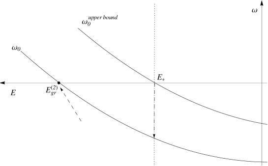
Figure 1: A Typical Flow of the First Eigenvalue of Principal Operator.

Therefore, by assuming that two-body problem is solved, we can then study n-body problem. Since we are only interested in the bound states of the model at the moment, we should be able to determine $n$-particle bound states after the renormalization procedure. The exact treatment of this problem is rather difficult. Assuming that the details of the two-body interaction can be understood, we will study the model in the mean field approximation in Section III. Before embarking on studying the mean field analysis, we will make some general remarks about the bound state spectrum of the problem.

It is a well known fact that the residue of the resolvent at its isolated pole $\mu$ is the projection operator $\mathbb{P}_{\mu}$ to the corresponding eigenspace of the Hamiltonian

$$\mathbb{P}_{\mu}=-{1\over 2\pi i}\oint_{\Gamma_{\mu}}\mathrm{d}E\;R(E)\;,$$ (92)

where $\Gamma_{\mu}$ is a small contour enclosing the isolated eigenvalue $\mu$ in the complex energy plane simon . Let us suppose that there exist a ground state and choose our contour enclosing this ground state energy, namely $E_{gr}$. Then, the above integral of $R(E)$ gives the projection to the eigenspace $|\Psi_{0}\rangle\langle\Psi_{0}|$ corresponding to the minimum eigenvalue of the renormalized Hamiltonian for the many-body system.

From (52), it is easily seen that the principal operator formally satisfies $\Phi^{{\dagger}}(E)=\Phi(E^{*})$. We assume that $\Phi(E)$ defines a self-adjoint holomorphic family of type A kato , so that we can apply the spectral theorem for the principal operator or inverse of it. Since the principal operator $\Phi(E)$ acts on $\mathcal{F_{B}}^{(n-2)}\otimes\mathcal{L}^{2}(\mathcal{M})$, we have

$$\Phi^{-1}(E)=\sum_{k}{1\over\omega_{k}(E)}\mathbb{P}_{k}(E)+\int_{\sigma}\mathrm{d}\omega(E)\;{1\over\omega(E)}\mathbb{P}_{\omega}(E)\;,$$ (93)

where the projection operator

$$\mathbb{P}_{k}(E)=|\phi_{k}(E)\rangle\langle\phi_{k}(E)|=|\omega_{k}(E);\Omega_{k}(E)\rangle\langle\omega_{k}(E);\Omega_{k}(E)|\;,$$ (94)

is given in terms of $n-2$ bosonic particle state and one-particle orthofermion state:

$$|\omega_{k}\rangle = \int_{\mathcal{M}^{n-2}}\mathrm{d}^{2}_{g}x_{1}\,\mathrm{d}^{2}_{g}x_{2}\ldots\mathrm{d}^{2}_{g}x_{n-2}\;u_{k}(x_{1},\ldots,x_{n-2})|x_{1}\ldots x_{n-2}\rangle$$ (95)

$$|\Omega_{k}\rangle = \int_{\mathcal{M}}\mathrm{d}^{2}_{g}x\;\psi_{k}(x)\chi^{{\dagger}}_{g}(x)|0\rangle\;.$$ (96)

Here $\omega_{k}(E)$ and $|\omega_{k}(E);\Omega_{k}(E)\rangle$ are the eigenvalues and the eigenvectors of the principal operator, respectively. Similarly, the (generalized) projection operator

$$\mathbb{P}_{\omega}(E) = |\phi(E)\rangle\langle\phi(E)|=|\omega(E);\Omega(E)\rangle\langle\omega(E);\Omega(E)|$$ (97)

corresponds to the continuous eigenvalues and eigenvectors of the principal operator. We assume that the principal operator has discrete as well as continuous eigenvalues and the bottom of the spectrum corresponds to a non-degenerate eigenvalue. Above integral is taken over the continuous spectrum $\sigma(\Phi)$ of the principal operator (for simplicity, we write it formally, it should be written more precisely as a Riemann-Stieltjies integral).

As emphasized in the previous section, the bound state spectrum corresponds to the solutions of the zero eigenvalues of the principal operator (52). In order to estimate the ground state energy of our system, it is crucial to determine how the eigenvalues $\omega_{k}$ evolve with $E$. For this purpose, let us calculate the derivative of the eigenvalue $\omega_{k}$ of the principal operator with respect to $E$. If we apply the Feynman-Hellman theorem to the eigenvalue problem for the principal operator, we get

$${\partial\omega_{k}\over\partial E}=\langle\phi_{k}|{\partial\Phi(E)\over\partial E}|\phi_{k}\rangle=\bigg{\langle}{\partial\Phi(E)\over\partial E}\bigg{\rangle}\;.$$ (98)

A direct computation for the derivative of the principal operator (52) with respect to the energy $E$ gives

$${\partial\Phi(E)\over\partial E}=-\Bigg{[}\int_{\mathcal{M}^{2}}\mathrm{d}_{g}^{2}x\,\mathrm{d}_{g}^{2}x^{\prime}\chi^{{\dagger}}_{g}(x)\int_{0}^{\infty}\mathrm{d}t\;t\;K_{t}^{2}(x,x^{\prime};g)e^{-t(H_{0}-E)}\chi_{g}(x^{\prime})+{1\over 2}\int_{\mathcal{M}^{6}}\mathrm{d}_{g}^{2}x\,\mathrm{d}_{g}^{2}x^{\prime}\,\mathrm{d}_{g}^{2}x_{1}\,\mathrm{d}_{g}^{2}x_{2}\,\mathrm{d}_{g}^{2}x^{\prime}_{1}\,\mathrm{d}_{g}^{2}x^{\prime}_{2}$$ (100)

$$\times\;\chi^{{\dagger}}_{g}(x)\,\chi_{g}(x^{\prime})\,\phi^{{\dagger}}_{g}(x^{\prime}_{1})\,\phi^{{\dagger}}_{g}(x^{\prime}_{2})\int_{0}^{\infty}\mathrm{d}t\;t\;K_{t}(x_{1},x;g)\,K_{t}(x_{2},x;g)\,K_{t}(x^{\prime},x^{\prime}_{1};g)\,K_{t}(x^{\prime},x^{\prime}_{2};g)\,e^{-t(H_{0}-E)}\phi_{g}(x_{1})\,\phi_{g}(x_{2})$$

$$\hskip 85.35826pt+2\int_{\mathcal{M}^{4}}\mathrm{d}_{g}^{2}x\,\mathrm{d}_{g}^{2}x^{\prime}\,\mathrm{d}_{g}^{2}x_{1}\,\mathrm{d}_{g}^{2}x_{2}\;\chi^{{\dagger}}_{g}(x)\,\chi_{g}(x^{\prime})\,\phi^{{\dagger}}_{g}(x_{1})\$$ (101)

$$\hskip 170.71652pt\times\int_{0}^{\infty}\mathrm{d}t\;t\,K_{t}(x_{2},x;g)\,K_{t}(x,x^{\prime};g)\,K_{t}(x^{\prime},x_{1};g)\,e^{-t(H_{0}-E)}\phi_{g}(x_{2})\Bigg{]}\;.$$ (102)

For simplicity, we will separate the terms in the expectation value of the principal operator in (98), using (102). Let us first consider the first term

$$\int_{\mathcal{M}^{2}}\mathrm{d}_{g}^{2}x\,\mathrm{d}_{g}^{2}x^{\prime}\;\psi^{*}(x)\int_{0}^{\infty}\mathrm{d}t\;t\;K_{t}^{2}(x,x^{\prime};g)\langle\omega_{k}|e^{-t(H_{0}-E)}|\omega_{k}\rangle\psi(x^{\prime})\;,$$ (103)

where $\psi(x)$ is the wave function of the orthofermion. If we think of the factor $t$ in the above integrand as an integral $\int_{-t}^{t}(\mathrm{d}u/2)$ and then make the change of variables $t=t_{1}+t_{2}$, $u=t_{1}-t_{2}$, we readily obtain

$$\int_{\mathcal{M}^{2}}\mathrm{d}_{g}^{2}x\,\mathrm{d}_{g}^{2}x^{\prime}\;\psi^{*}(x)\int_{0}^{\infty}\int_{0}^{\infty}\;\mathrm{d}t_{1}\,\mathrm{d}t_{2}\;\;K_{t_{1}+t_{2}}^{2}(x,x^{\prime};g)\langle\omega_{k}|e^{-(t_{1}+t_{2})(H_{0}-E)}|\omega_{k}\rangle\psi(x^{\prime})\;.$$ (104)

Using the semi-group property of the heat kernel (40), equation (104) can be rewritten as

$$\hskip-28.45274pt\int_{\mathcal{M}^{2}}\mathrm{d}_{g}^{2}x\,\mathrm{d}_{g}^{2}x^{\prime}\;\psi^{*}(x)\int_{0}^{\infty}\int_{0}^{\infty}\;\mathrm{d}t_{1}\,\mathrm{d}t_{2}\;\int_{\mathcal{M}^{2}}\mathrm{d}_{g}^{2}z_{1}\,\mathrm{d}_{g}^{2}z_{2}\;K_{t_{1}}(x,z_{1};g)K_{t_{2}}(z_{1};x^{\prime};g)K_{t_{1}}(x,z_{2};g)$$ (105)

$$\hskip 142.26378pt\times\;K_{t_{2}}(z_{2},x^{\prime};g)\langle\omega_{k}|e^{-(t_{1}+t_{2})(H_{0}-E)}|\omega_{k}\rangle\psi(x^{\prime})\;.$$ (106)

Changing the order of integrations we find

$$\int_{\mathcal{M}^{2}}\mathrm{d}_{g}^{2}z_{1}\,\mathrm{d}_{g}^{2}z_{2}\;\Bigg{|}\Bigg{|}\int_{0}^{\infty}\;\mathrm{d}t_{1}\;e^{-t_{1}(H_{0}-E)}\int_{\mathcal{M}}\mathrm{d}_{g}^{2}x\;K_{t_{1}}(z_{1},x;g)K_{t_{1}}(x,z_{2};g)\psi^{*}(x)|\omega_{k}\rangle\Bigg{|}\Bigg{|}^{2}\;,$$ (107)

which is obviously always positive. Now we return to the expectation value of the second and third terms in (102). It is easy to see that they can be expressed as

$${1\over 2}\int_{0}^{\infty}\mathrm{d}t\;t\,\Bigg{|}\Bigg{|}\int_{\mathcal{M}^{3}}\mathrm{d}_{g}^{2}x_{1}\,\mathrm{d}_{g}^{2}x_{2}\,\mathrm{d}_{g}^{2}x\;K_{t}(x_{1},x;g)K_{t}(x,x_{2};g)\psi^{*}(x)\;e^{-{t\over 2}(H_{0}-E)}\phi_{g}(x_{1})\phi_{g}(x_{2})|\omega_{k}\rangle\Bigg{|}\Bigg{|}^{2}$$ (108)

$$\hskip-14.22636pt+\;2\int_{\mathcal{M}}\mathrm{d}_{g}^{2}z\int_{0}^{\infty}\mathrm{d}t\;t\,\Bigg{|}\Bigg{|}\int_{\mathcal{M}^{2}}\mathrm{d}_{g}^{2}x\,\mathrm{d}_{g}^{2}x_{2}\;K_{t/2}(z,x;g)K_{t}(x,x_{2};g)\psi^{*}(x)\;e^{-{t\over 2}(H_{0}-E)}\phi_{g}(x_{2})|\omega_{k}\rangle\Bigg{|}\Bigg{|}^{2}\;,$$ (109)

where we have used the fact that we can rewrite the second heat kernel $K_{t}(x,x^{\prime};g)$ in the third term of (102) as $\int_{\mathcal{M}}\mathrm{d}_{g}^{2}z\;K_{t/2}(x,z;g)K_{t/2}(z,x^{\prime};g)$ by the semi-group property (40). Consequently, we obtain

$${\partial\omega_{k}\over\partial E}<0\;.$$ (110)

The eigenvalues $\omega_{k}(E)$’s flow with $E$ in accordance with (110), that is, these are monotonically decreasing functions of $E$. For sufficiently small values of $E$, there can not be a zero eigenvalue of the principal operator since the energy must be bounded from below. Moreover, for a given $E_{*}$ the eigenvalues can be ordered as $\omega_{0}(E_{*})<\omega_{1}(E_{*})<\ldots$. Therefore, due to (110) and non-degeneracy of the lowest eigenvalue $\omega_{0}$, only the minimum eigenvalue $\omega_{0}$ flows to its zero value at the minimum energy $E=E_{gr}$. Hence, the ground state corresponds to the zero of the minimum eigenvalue $\omega_{0}(E)$ of $\Phi(E)$, as shown in Figure 2.

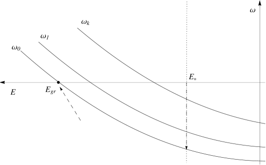
Figure 2: A Typical Flow of the Eigenvalues of Principal Operator.

We may now show that $E^{(n)}_{gr}\leq E^{(2)}_{gr}$ for compact manifolds. To see this, we take the solution of two-body ground state $|\Psi^{(2)}\rangle$ as

$$|\Psi^{(2)}\rangle=|0\rangle\otimes\int_{\mathcal{M}}\mathrm{d}_{g}x\;\psi_{0}^{(2)}(x)\chi^{{\dagger}}(x)|0\rangle$$ (111)

and then make a new ansatz $|\Psi^{var}\rangle$ for the $n$-body problem in the form

$$|\Psi^{var}\rangle={1\over[V(\mathcal{M})]^{(n-2)/2}}\int_{\mathcal{M}^{n-2}}\mathrm{d}_{g}x_{1}\;\ldots\mathrm{d}_{g}x_{n-2}|x_{1},\ldots,x_{n-2}\rangle\otimes\int_{\mathcal{M}}\mathrm{d}_{g}x\;\psi_{0}^{(2)}(x)\chi^{{\dagger}}(x)|0\rangle\;.$$ (112)

It is convenient to split the principal operator $\Phi(E)$ given in (52) as $K(E)-U(E)$, where

$$K(E)=\int_{\mathcal{M}^{2}}\mathrm{d}_{g}^{2}x\,\mathrm{d}_{g}^{2}x^{\prime}\chi^{{\dagger}}_{g}(x)\int_{0}^{\infty}\mathrm{d}t\;\bigg{[}{e^{-t\mu^{2}}\over 8\pi t}\delta_{g}^{(2)}(x,x^{\prime})-K_{t}^{2}(x,x^{\prime};g)e^{-t(H_{0}-E)}\bigg{]}\chi_{g}(x^{\prime})$$ (113)

and

$$\hskip-56.9055ptU(E)={1\over 2}\int_{0}^{\infty}\mathrm{d}t\;\bigg{[}\int_{\mathcal{M}^{3}}\mathrm{d}_{g}^{2}x\,\mathrm{d}_{g}^{2}x_{1}\,\mathrm{d}_{g}^{2}x_{2}\,K_{t}(x_{1},x;g)\,K_{t}(x,x_{2};g)\,\phi_{g}(x_{1})\,\phi_{g}(x_{2})\,\chi_{g}(x)\bigg{]}^{{\dagger}}e^{-t(H_{0}-E)}$$ (114)

$$\hskip 85.35826pt\times\;\bigg{[}\int_{\mathcal{M}^{3}}\mathrm{d}_{g}^{2}x^{\prime}\,\mathrm{d}_{g}^{2}x^{\prime}_{1}\,\mathrm{d}_{g}^{2}x^{\prime}_{2}\,K_{t}(x^{\prime}_{1},x^{\prime};g)\,K_{t}(x^{\prime},x^{\prime}_{2};g)\,\phi_{g}(x^{\prime}_{1})\,\phi_{g}(x^{\prime}_{2})\,\chi_{g}(x^{\prime})\bigg{]}$$ (115)

$$+\,2\int_{\mathcal{M}}\mathrm{d}_{g}^{2}z\;\int_{0}^{\infty}\mathrm{d}t\;\bigg{[}\int_{\mathcal{M}^{2}}\mathrm{d}_{g}^{2}x\,\mathrm{d}_{g}^{2}x_{1}\,K_{t}(x_{1},x;g)\,K_{t/2}(x,z;g)\,\phi_{g}(x_{1})\chi_{g}(x)\bigg{]}^{{\dagger}}e^{-t(H_{0}-E)}$$ (116)

$$\hskip 85.35826pt\times\;\bigg{[}\int_{\mathcal{M}^{2}}\mathrm{d}_{g}^{2}x^{\prime}\,\mathrm{d}_{g}^{2}x^{\prime}_{1}\,K_{t}(x^{\prime}_{1},x^{\prime};g)\,K_{t/2}(x^{\prime},z;g)\,\phi_{g}(x^{\prime}_{1})\chi_{g}(x^{\prime})\bigg{]}\;,$$ (117)

where we have used the semi-group property of heat kernel (40) and the assumption that we can interchange the order of integrations. By the variational principle,

$$\omega_{0}^{(n)}(E_{gr}^{(2)})\leq\langle\Psi^{var}|\Phi(E_{gr}^{(2)})|\Psi^{var}\rangle=-\langle\Psi^{var}|U(E_{gr}^{(2)})|\Psi^{var}\rangle\;,$$ (118)

where $\langle\psi_{0}^{(2)}|K(E^{(2)}_{gr})|\psi_{0}^{(2)}\rangle=0$. In order to calculate the above expectation value, we first show that

$$e^{-{t\over 2}(H_{0}-E)}\int_{\mathcal{M}^{3}}\mathrm{d}_{g}^{2}x^{\prime}\,\mathrm{d}_{g}^{2}x^{\prime}_{1}\,\mathrm{d}_{g}^{2}x^{\prime}_{2}\,K_{t}(x^{\prime}_{1},x^{\prime};g)\,K_{t}(x^{\prime},x^{\prime}_{2};g)\,\phi_{g}(x^{\prime}_{1})\,\phi_{g}(x^{\prime}_{2})\,\chi_{g}(x^{\prime})|\Psi^{var}\rangle$$ (119)

$$={(n-2)^{1/2}(n-3)^{1/2}\over[V(\mathcal{M})]^{(n-2)/2}}e^{-{t\over 2}|E_{gr}^{(2)}|}\int_{\mathcal{M}^{3}}\mathrm{d}_{g}^{2}x^{\prime}\,\mathrm{d}_{g}^{2}x^{\prime}_{1}\,\mathrm{d}_{g}^{2}x^{\prime}_{2}\,K_{t}(x^{\prime}_{1},x^{\prime};g)\,K_{t}(x^{\prime},x^{\prime}_{2};g)\psi_{0}^{(2)}(x^{\prime})$$ (120)

$$\hskip 142.26378pt\times\;\int_{\mathcal{M}^{n-4}}\mathrm{d}_{g}y_{3}\;\ldots\mathrm{d}_{g}y_{n-2}|y_{3},\ldots,y_{n-2}\rangle$$ (121)

$$={(n-2)^{1/2}(n-3)^{1/2}\over[V(\mathcal{M})]^{(n-2)/2}}e^{-{t\over 2}|E_{gr}^{(2)}|}\int_{\mathcal{M}}\mathrm{d}_{g}^{2}x^{\prime}\,\psi_{0}^{(2)}(x^{\prime})\int_{\mathcal{M}^{n-4}}\mathrm{d}_{g}y_{3}\;\ldots\mathrm{d}_{g}y_{n-2}|y_{3},\ldots,y_{n-2}\rangle\;,$$ (122)

where we have used the fact that the free Hamiltonian operates on bosonic states and gives zero for constant wave functions. We have also used the stochastic completeness of the heat kernel in the last line. Then, the expectation value of the first term in (117) becomes

$${(n-2)(n-3)\over 2}\int_{0}^{\infty}\mathrm{d}t\;e^{-t|E_{gr}^{(2)}|}\bigg{|}\int_{\mathcal{M}}\mathrm{d}_{g}^{2}x\,\psi_{0}^{(2)}(x)\bigg{|}^{2}{[V(\mathcal{M})]^{(n-4)}\over[V(\mathcal{M})]^{(n-2)}}\;,$$ (123)

which is finite due to

$$\bigg{|}\int_{\mathcal{M}}\mathrm{d}_{g}^{2}x\,\psi_{0}^{(2)}(x)\bigg{|}^{2}\leq\bigg{[}\int_{\mathcal{M}}\mathrm{d}_{g}^{2}x\,|\psi_{0}^{(2)}(x)|^{2}\bigg{]}\bigg{[}\int_{\mathcal{M}}\mathrm{d}_{g}^{2}x\bigg{]}=V(\mathcal{M})\;.$$ (124)

Similarly, we can calculate the expectation value of the second term in (117) and get

$${2(n-2)\over V(\mathcal{M})}\int_{0}^{\infty}\mathrm{d}t\;\Bigg{[}\int_{\mathcal{M}}\mathrm{d}_{g}^{2}z\,\bigg{|}\int_{\mathcal{M}}\mathrm{d}_{g}^{2}x\,K_{t/2}(x,z;g)\psi_{0}^{(2)}(x)\bigg{|}^{2}\Bigg{]}e^{-t|E_{gr}^{(2)}|}\;.$$ (125)

It can be shown that the above integral is finite if we use the eigenfunction expansions (29) and (33), so that we have

$$\int_{\mathcal{M}}\mathrm{d}_{g}^{2}z\,\bigg{|}\int_{\mathcal{M}}\mathrm{d}_{g}^{2}x\,K_{t/2}(x,z;g)\psi_{0}^{(2)}(x)\bigg{|}^{2}=\Bigg{[}\int_{\mathcal{M}}\mathrm{d}_{g}^{2}z\,\bigg{|}\bigg{|}e^{{t\over 2}\nabla_{g}^{2}}|\psi_{0}^{(2)}\rangle\bigg{|}\bigg{|}^{2}\Bigg{]}=\sum_{l}e^{-t\sigma_{l}}|\tilde{\psi}_{0}^{(2)}(l)|^{2}\;,$$ (126)

where $\psi_{0}^{(2)}(x)=\sum_{l}f_{l}(x;g)\tilde{\psi}_{0}^{(2)}(l)$. Since $\sum_{l}e^{-t\sigma_{l}}|\tilde{\psi}_{0}^{(2)}(l)|^{2}\leq e^{-t\sigma_{0}}\sum_{l}|\tilde{\psi}_{0}^{(2)}(l)|^{2}$ and the minimum eigenvalue $\sigma_{0}=0$ for compact manifolds, the above integral is bounded from above by $1$ and so that equation (125) is finite. Hence, we obtain

$$\omega_{0}^{(n)}(E_{gr}^{(2)})\leq-{(n-2)(n-3)\over 2|E_{gr}^{(2)}|[V(\mathcal{M})]^{2}}\bigg{|}\int_{\mathcal{M}}\mathrm{d}_{g}^{2}x\,\psi_{0}^{(2)}(x)\bigg{|}^{2}$$ (127)

$$\hskip 113.81102pt-{2(n-2)\over V(\mathcal{M})}\int_{0}^{\infty}\mathrm{d}t\;\Bigg{[}\int_{\mathcal{M}}\mathrm{d}_{g}^{2}z\,\bigg{|}\int_{\mathcal{M}}\mathrm{d}_{g}^{2}x\,K_{t/2}(x,z;g)\psi_{0}^{(2)}(x)\bigg{|}^{2}\Bigg{]}e^{-t|E_{gr}^{(2)}|}<0\;.$$ (128)

As a consequence of (110) and (128), to find the zero of $\omega_{0}(E)$ in the $n$-particle sector we must reduce $E$ below $E_{gr}^{(2)}$, as shown in Figure 3. This completes the proof.

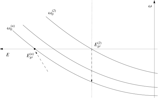
Figure 3: A Typical Flow of the Eigenvalues of Principal Operator in the two and $n$-boson sector.

We will now calculate $n$-particle ground state wave function in terms of the solution $|\phi_{0}\rangle$ of $\Phi(E_{gr})|\phi_{0}\rangle=0$.

Let us expand the minimum eigenvalue $\omega_{0}(E)$ near the bound state energy $E_{gr}$

$$\omega_{0}(E)=\omega_{0}(E_{gr})+(E-E_{gr}){\partial\omega_{0}(E)\over\partial E}\bigg{|}_{E_{gr}}+\cdots=(E-E_{gr}){\partial\omega_{0}(E)\over\partial E}\bigg{|}_{E_{gr}}+\cdots\;.$$ (129)

Using this result and (93), equation (92) yields

$${1\over 2}(H_{0}-E_{gr})^{-1}\int_{\mathcal{M}}\mathrm{d}_{g}^{2}x\;\phi^{{\dagger}}_{g}(x)\phi^{{\dagger}}_{g}(x)\psi_{0}(x)\left(-{\partial\omega_{0}(E)\over\partial E}\bigg{|}_{E_{gr}}\right)^{-1}|\omega_{0}(E_{gr})\rangle\langle\omega_{0}(E_{gr})|$$ (130)

$$\hskip 256.0748pt\times\int_{\mathcal{M}}\mathrm{d}_{g}^{2}y\;\phi_{g}(y)\phi_{g}(y)\psi^{*}_{0}(y)(H_{0}-E_{gr})^{-1}\;.$$ (131)

We assume that there is no other pole coming from $(H_{0}-E)^{-1}$ near $E_{gr}$, and no other terms for $k\neq 0$ contribute to the integral around $E=E_{gr}$. Let the eigenvector of the principal operator corresponding to the ground state be

$$|\phi_{0}(E_{gr})\rangle=\int_{\mathcal{M}^{n-2}}\mathrm{d}_{g}^{2}x_{1}\cdots\mathrm{d}_{g}^{2}x_{n-2}\;u_{0}(x_{1},\cdots,x_{n-2})|x_{1}\cdots x_{n-2}\rangle\int_{\mathcal{M}}\mathrm{d}_{g}^{2}x\;\psi_{0}(x)\chi^{\dagger}_{g}(x)|0\rangle\;.$$ (132)

By using the eigenfunction expansion of the creation and the annihilation operators and their commutation relations, we will shift all creation operators $\phi^{{\dagger}}_{g}(x)$ in (131) coming from (132) to the leftmost

$${1\over H_{0}-E}\phi^{{\dagger}}_{g}(x)\phi^{{\dagger}}_{g}(x)\phi^{{\dagger}}_{g}(x_{1})\cdots\phi^{{\dagger}}_{g}(x_{n-2})=\int_{\mathcal{M}^{n}}\mathrm{d}_{g}^{2}y_{1}\cdots\mathrm{d}_{g}^{2}y_{n}\;\phi^{{\dagger}}_{g}(y_{1})\cdots\phi^{{\dagger}}_{g}(y_{n})$$ (133)

$$\hskip 113.81102pt\times\int_{0}^{\infty}\mathrm{d}t\;e^{-t(H_{0}-E)}\,K_{t}(y_{1},x;g)K_{t}(y_{2},x;g)K_{t}(y_{3},x_{1};g)\cdots K_{t}(y_{n},x_{n-2};g)\;,$$ (134)

and all annihilation operators $\phi_{g}(x)$ in (131) coming from (132) to the rightmost

$$\phi_{g}(x)\phi_{g}(x)\phi_{g}(x_{1})\cdots\phi_{g}(x_{n-2}){1\over H_{0}-E}=\int_{\mathcal{M}^{n}}\mathrm{d}_{g}^{2}y_{1}\cdots\mathrm{d}_{g}^{2}y_{n}\;\int_{0}^{\infty}\mathrm{d}t\;e^{-t(H_{0}-E)}$$ (135)

$$\hskip 113.81102pt\times\;K_{t}(y_{1},x;g)K_{t}(y_{2},x;g)K_{t}(y_{3},x_{1};g)\cdots K_{t}(y_{n},x_{n-2};g)\phi_{g}(y_{1})\cdots\phi_{g}(y_{n})\;,$$ (136)

which are the generalized versions of equations we first used in nrleemodelonmanifold . Therefore, from equation (131), we read the state vector $|\Psi_{0}\rangle$ of our many-body system in terms of the eigenstate $|\phi_{0}\rangle$ of the principal operator

$$|\Psi_{0}\rangle=\int_{\mathcal{M}^{n}}\mathrm{d}_{g}^{2}y_{1}\cdots\mathrm{d}_{g}^{2}y_{n}\;\Psi_{0}(y_{1},\ldots,y_{n})|y_{1}\cdots y_{n}\rangle$$ (137)

$$={1\over\sqrt{2}}\int_{\mathcal{M}^{n}}\mathrm{d}_{g}^{2}y_{1}\cdots\mathrm{d}_{g}^{2}y_{n}\;\int_{\mathcal{M}^{n-1}}\mathrm{d}_{g}^{2}x_{1}\cdots\mathrm{d}_{g}^{2}x_{n-2}\mathrm{d}_{g}^{2}x\;{1\over n!}\sum_{\sigma\in[1\cdots n]}\int_{0}^{\infty}\mathrm{d}t\;e^{-t|E_{gr}|}K_{t}(y_{\sigma(1)},x;g)K_{t}(y_{\sigma(2)},x;g)$$ (138)

$$\hskip 28.45274pt\times\;K_{t}(y_{\sigma(3)},x_{1};g)\cdots K_{t}(y_{\sigma(n)},x_{n-2};g)\;u_{0}(x_{1},\cdots,x_{n-2})\psi_{0}(x)\left(-{\partial\omega_{0}(E)\over\partial E}\bigg{|}_{E_{gr}}\right)^{-1/2}|y_{1}\cdots y_{n}\rangle\;,$$ (139)

where the sum runs over all permutations $\sigma$ of $[123\ldots n]$. Comparing equation (132) and equation (139), we see that the state $|\Psi_{0}\rangle$ is a complicated convoluted integral of the eigenstate $|\phi_{0}\rangle$ with the heat kernels.

III Mean Field Approximation

In standard quantum field theory, one expects that all the bosons have the same wave function $u(x)$ for the limit of large number of bosons, i.e., as $n\rightarrow\infty$ and the wave function of the system has the product form of the one-particle wave functions. However, due to the singular structure of our problem, the wave function in (139) can not have a product form in the large $n$ limit. In order to see this, we scale $t=t^{\prime}/|E_{gr}|$. With a hindsight coming from the proof that the lower bound of the ground state energy grows exponentially with the number of bosons in flat space rajeevbound ; rajeevdimock we may assume that $E_{gr}$ grows fast enough as $n$ increases. In this case, all integrals of the heat kernels are peaked around $y_{\sigma(k)}$. (This is clear from (10) and also from the stochastic completeness assumption). Then, all integrals of $x_{l}$ are

$$\int_{\mathcal{M}}\mathrm{d}_{g}^{2}x_{l}\;K_{t/|E_{gr}|}(x_{l},y_{\sigma(l+1)})u_{0}(x_{1},\ldots,x_{l},\ldots,x_{n-2})\approx u_{0}(x_{1},\ldots,y_{\sigma(l+1)},\ldots,x_{n-2})\;,$$ (140)

for $l=1,\ldots,n-2$ as $n\rightarrow\infty$ and similarly for $x$ integral. Then, the state $|\Psi_{0}\rangle$ becomes

$$|\Psi_{0}\rangle\approx{1\over\sqrt{2}}\int_{\mathcal{M}^{n}}\mathrm{d}_{g}^{2}y_{1}\cdots\mathrm{d}_{g}^{2}y_{n}\;{1\over n!}\sum_{\sigma\in[1\cdots n]}\int_{0}^{\infty}\mathrm{d}t\;e^{-t|E_{gr}|}K_{t}(y_{\sigma(1)},y_{\sigma(2)};g)$$ (141)

$$\hskip 142.26378pt\times\;u_{0}(y_{\sigma(3)},\cdots,y_{\sigma(n)})\psi_{0}(y_{\sigma(2)})\left(-{\partial\omega_{0}(E)\over\partial E}|_{E_{gr}}\right)^{-1/2}|y_{1}\cdots y_{n}\rangle\;.$$ (142)

One can understand the singular nature of the wave function in this limiting form more easily. We pick any two bosons, and transform them through our formalism into an orthofermion, with its wave function $\psi_{0}$ to be determined consistently. This orthofermion wave function corresponding to the pairing, could be quite regular, yet its multiplication with the heat kernel, integrated over the time variable produces a function singular as the two variables of the heat kernel approach to one another. This singularity is the same as the singularity of the bound state wave function of a particle interacting with a delta source ermanturgut , hence it is square integrable.

It is important to notice that $|\Psi_{0}\rangle$ is not in the domain of $H_{0}$. To prove this, it is sufficient to consider the following term which appears in calculating $\langle\Psi_{0}|H_{0}|\Psi_{0}\rangle$

$$\hskip-14.22636pt\int_{\mathcal{M}^{2}}\mathrm{d}^{2}_{g}x\,\mathrm{d}^{2}_{g}y\;\int_{0}^{\infty}\mathrm{d}t_{1}\;e^{-t_{1}|E_{gr}|}K_{t_{1}}(x,y;g)\psi_{0}(y)\Bigg{[}\int_{0}^{\infty}\mathrm{d}t_{2}\;e^{-t_{2}|E_{gr}|}\left(-{1\over 2m}\right)\nabla_{g}^{2}K_{t_{2}}(x,y;g)\Bigg{]}$$ (143)

$$=\int_{\mathcal{M}^{2}}\mathrm{d}^{2}_{g}x\,\mathrm{d}^{2}_{g}y\;\int_{0}^{\infty}\mathrm{d}t_{1}\;e^{-t_{1}|E_{gr}|}K_{t_{1}}(x,y;g)\psi_{0}(y)\Bigg{[}\int_{0}^{\infty}\mathrm{d}t_{2}\;e^{-t_{2}|E_{gr}|}\bigg{(}-{\partial K_{t_{2}}(x,y;g)\over\partial t_{2}}\bigg{)}\Bigg{]}\;,$$ (144)

where we have used the fact that the heat kernel satisfies the heat equation (9). After applying the integration by parts to the $t_{2}$ integral and using the initial condition for the heat kernel $K_{t}(x,y;g)\rightarrow\delta_{g}(x,y)$ as $t\rightarrow 0^{+}$ and (40), we find

$$\int_{\mathcal{M}^{2}}\mathrm{d}^{2}_{g}x\,\mathrm{d}^{2}_{g}y\;\int_{0}^{\infty}\mathrm{d}t_{1}\;e^{-t_{1}|E_{gr}|}K_{t_{1}}(x,y;g)\psi_{0}(y)\Bigg{[}\delta_{g}(x,y)-|E_{gr}|\int_{0}^{\infty}\mathrm{d}t_{2}\;e^{-t_{2}|E_{gr}|}K_{t_{2}}(x,y;g)\Bigg{]}$$ (145)

$$=\int_{\mathcal{M}}\mathrm{d}^{2}_{g}x\;\int_{0}^{\infty}\mathrm{d}t_{1}\;e^{-t_{1}|E_{gr}|}K_{t_{1}}(x,x;g)\psi_{0}(x)$$ (146)

$$\hskip 113.81102pt-|E_{gr}|\int_{0}^{\infty}\mathrm{d}t_{1}\;e^{-t_{1}|E_{gr}|}\int_{\mathcal{M}}\mathrm{d}^{2}_{g}x\;\int_{0}^{\infty}\mathrm{d}t_{2}\;e^{-t_{2}|E_{gr}|}K_{t_{1}+t_{2}}(x,x;g)\psi_{0}(x)\;.$$ (147)

After the change of variables $u=t_{1}+t_{2}$ and $v=t_{1}-t_{2}$, we get

$$\hskip-28.45274pt\int_{\mathcal{M}}\mathrm{d}^{2}_{g}x\;\psi_{0}(x)\Bigg{[}\int_{0}^{\infty}\mathrm{d}t_{1}\;e^{-t_{1}|E_{gr}|}K_{t_{1}}(x,x;g)-|E_{gr}|\int_{0}^{\infty}\mathrm{d}u\;u\;e^{-u|E_{gr}|}K_{u}(x,x;g)\Bigg{]}\;.$$ (148)

The first term is divergent due to (47). Similar to the problem with point interactions on manifolds which we studied in ermanturgut , our problem here can also be considered as a kind of self-adjoint extension since the state $\Psi_{0}$ does not belong to the domain of the free Hamiltonian. The self-adjoint extension of the free Hamiltonian extends this domain such that the state $\Psi_{0}$ is included. Although the state $\Psi_{0}$ is not in the domain of $H_{0}$, the eigenvector corresponding to the eigenfunction $u_{0}(x)$ for the lowest eigenvalue of $\Phi(E)$ can be taken in the domain of $H_{0}$.

As a result, $|\Psi_{0}\rangle$ given in (142) is not in the product form in the large $n$ limit, that is,

$$|\Psi_{0}\rangle\neq\int_{\mathcal{M}^{n}}\mathrm{d}_{g}^{2}y_{1}\cdots\mathrm{d}_{g}^{2}y_{n}\;\prod_{k=1}^{n}\Psi_{0}(y_{k})|y_{1}\cdots y_{n}\rangle\;.$$ (149)

The solution takes a kind of convolution of the wave functions in the domain of $H_{0}$ with the bound state wave function which is outside of this domain.

Yet, $\Phi(E)$’s lowest eigenfunction may well be approximated by a product form for large number of bosons, that is,

$$u_{0}(x_{1},\cdots,x_{n-2})=u_{0}(x_{1})\cdots u_{0}(x_{n-2})\;,$$ (150)

with the normalization

$$||u_{0}||^{2}=\int_{\mathcal{M}}\mathrm{d}_{g}^{2}x\;|u_{0}(x)|^{2}=1\;,\int_{\mathcal{M}}\mathrm{d}_{g}^{2}x\;|\psi_{0}(x)|^{2}=1\;.$$ (151)

Therefore, the expectation value of the principal operator by applying the mean field ansatz must vanish, that is,

$$\langle\phi_{0}|\Phi(E_{gr})|\phi_{0}\rangle=0\;.$$ (152)

Although such a mean field approximation is expected to be crude in less than three dimensions, F. Calogero and A. Degasperis calogero have shown that even in one dimension the mean field approach to this problem gives an excellent agreement with the exact result. This is a finite problem and we will see in the next subsection that the present approach is also consistent with the exact result. Therefore, we expect that the mean field approximation to this problem in two-dimensions is also reliable.

In order to calculate (152) explicitly, we will make normal ordering of the creation and the annihilation operators by using their eigenfunction expansion. Hence, the equation above yields

$$\int_{0}^{\infty}\mathrm{d}t\;\Bigg{[}{e^{-t\mu^{2}}\over 8\pi t}-\int_{\mathcal{M}^{2}}\mathrm{d}_{g}^{2}x\,\mathrm{d}_{g}^{2}y\;\psi_{0}^{*}(x)\psi_{0}(y)K_{t}^{2}(x,y;g)e^{-t|E_{gr}|}\bigg{(}\int_{\mathcal{M}^{2}}\mathrm{d}_{g}^{2}x^{\prime}\,\mathrm{d}_{g}^{2}y^{\prime}\;u_{0}^{*}(x^{\prime})K_{t}(x^{\prime},y^{\prime};g)u_{0}(y^{\prime})\bigg{)}^{n-2}\Bigg{]}$$ (154)

$$={(n-2)(n-3)\over 2}\int_{0}^{\infty}\mathrm{d}t\;\Bigg{|}\int_{\mathcal{M}^{3}}\mathrm{d}_{g}^{2}x\,\mathrm{d}_{g}^{2}x_{1}\,\mathrm{d}_{g}^{2}x_{2}\;u_{0}^{*}(x_{1})u_{0}^{*}(x_{2})K_{t}(x_{1},x;g)\,K_{t}(x_{2},x;g)\psi_{0}(x)\Bigg{|}^{2}$$

$$\hskip 227.62204pt\times\;e^{-t|E_{gr}|}\bigg{(}\int_{\mathcal{M}^{2}}\mathrm{d}_{g}^{2}x^{\prime}\,\mathrm{d}_{g}^{2}y^{\prime}\;u_{0}^{*}(x^{\prime})K_{t}(x^{\prime},y^{\prime};g)u_{0}(y^{\prime})\bigg{)}^{n-4}$$ (157)

$$+\,2(n-2)\int_{0}^{\infty}\mathrm{d}t\;\Bigg{|}\int_{\mathcal{M}^{2}}\mathrm{d}_{g}^{2}x\,\mathrm{d}_{g}^{2}y\;u_{0}^{*}(x)K_{t}(x,y;g)\psi_{0}(y)\Bigg{|}^{2}e^{-t|E_{gr}|}$$

$$\hskip 227.62204pt\times\;\bigg{(}\int_{\mathcal{M}^{2}}\mathrm{d}_{g}^{2}x^{\prime}\,\mathrm{d}_{g}^{2}y^{\prime}\;u_{0}^{*}(x^{\prime})K_{t}(x^{\prime},y^{\prime};g)u_{0}(y^{\prime})\bigg{)}^{n-3}\;.$$

We are going to approximately solve $E_{gr}$ from the above equality for large values of $n$. In order to solve it, we may assume that $|E_{gr}|$ grows rapidly with $n$. This is plausible because $|E_{gr}|\simeq\mu^{2}e^{\pi n/6}$ for flat space $\mathbb{R}^{2}$ given in the mean field approximation rajeevbound . Every Riemannian manifold can locally be considered as a flat space, and the infinity appears due to the high values of momenta (ultraviolet divergence) or short distances we expect that the result for the large $n$ behavior of the ground state energy is similar on the manifold case. This allows us to consider the above equality in the large values $|E_{gr}|\gg\mu^{2}$ so our aim is to find only the terms that contribute most to the above integrals.

We first calculate asymptotically the left hand side of (157)

$$\hskip-14.22636pt\int_{0}^{\infty}\mathrm{d}t\;\Bigg{[}{e^{-t\mu^{2}}\over 8\pi t}-\int_{\mathcal{M}^{2}}\mathrm{d}_{g}^{2}x\,\mathrm{d}_{g}^{2}y\;\psi_{0}^{*}(x)\psi_{0}(y)K_{t}^{2}(x,y;g)e^{-t|E_{gr}|}\bigg{(}\int_{\mathcal{M}^{2}}\mathrm{d}_{g}^{2}x^{\prime}\,\mathrm{d}_{g}^{2}y^{\prime}\;u_{0}^{*}(x^{\prime})K_{t}(x^{\prime},y^{\prime};g)u_{0}(y^{\prime})\bigg{)}^{n}\Bigg{]}\;,$$ (158)

for the large values of $|E_{gr}|$. We will now ignore the additive constants to $n$, e.g., $n-2\simeq n$ since $n$ is very large. The major contribution to the above integral for large values of $|E_{gr}|$ can be computed since the asymptotic expansion of the following form, namely Laplace integrals

$$I(|E_{gr}|)=\int_{a}^{b}\mathrm{d}t\;f(t)e^{-|E_{gr}|g(t)}\;,$$ (159)

is given by Watson’s Lemma bender . The main contribution to the above integral can be obtained by Taylor or when necessary by the asymptotic expansions of the functions $f(t)$ and $g(t)$ near the minimum of $g(t)$. Similar to the reasoning given in the previous section, we write the square of the heat kernel in a subtle way, that is, we will use the initial condition for one of the heat kernels near $t=0$. After this and an integration, we substitute the asymptotic expansion (47) for the diagonal heat kernel near $t=0$ (the region that gives the dominant contribution). Hence, the left hand side for large values of $|E_{gr}|\gg\mu^{2}$ becomes

$$\int_{0}^{\infty}\mathrm{d}t\;\Bigg{[}{e^{-t\mu^{2}}\over 8\pi t}-\int_{\mathcal{M}}\mathrm{d}_{g}^{2}x\;|\psi_{0}(x)|^{2}{e^{-t|E_{gr}|}\over 8\pi t}\bigg{(}\int_{\mathcal{M}}\mathrm{d}_{g}^{2}x^{\prime}\;|u_{0}(x^{\prime})|^{2}\bigg{)}^{n}\Bigg{]}$$ (160)

$$=\int_{0}^{\infty}\mathrm{d}t\;\Bigg{[}{e^{-t\mu^{2}}\over 8\pi t}-{e^{-t|E_{gr}|}\over 8\pi t}\Bigg{]}={1\over 8\pi}\ln(|E_{gr}|/\mu^{2})\;.$$ (161)

As for the right hand side of (157), we apply the same method while we keep the next order terms coming from the eigenfunction expansion of the heat kernel in the $n$-th power of the integrals. Therefore, we obtain

$${n^{2}\over 2}\int_{0}^{\infty}\mathrm{d}t\;\Bigg{|}\int_{\mathcal{M}}\mathrm{d}_{g}^{2}x\;|u_{0}(x)|^{2}\psi_{0}(x)\Bigg{|}^{2}e^{-t|E_{gr}|}\bigg{(}\int_{\mathcal{M}}\mathrm{d}_{g}^{2}x\;|u_{0}(x)|^{2}-tK[u_{0}]\bigg{)}^{n}$$ (162)

$$\hskip 113.81102pt+\,2n\int_{0}^{\infty}\mathrm{d}t\;\Bigg{|}\int_{\mathcal{M}}\mathrm{d}_{g}^{2}x\;u_{0}^{*}(x)\psi_{0}(x)\Bigg{|}^{2}e^{-t|E_{gr}|}\bigg{(}\int_{\mathcal{M}}\mathrm{d}_{g}^{2}x\;|u_{0}(x)|^{2}-tK[u_{0}]\bigg{)}^{n}\;,$$ (163)

where we have defined

$$K[u_{0}]=\int_{\mathcal{M}}\mathrm{d}_{g}^{2}x\;|\nabla_{g}u_{0}(x)|^{2}\;,$$ (164)

and used the eigenfunction expansion of the heat kernel (33) and expanded the exponential inside by keeping the first two terms:

$$K_{t}(x,y;g)\approx\sum_{l}\left(1-t\sigma_{l}\right)f_{l}(x;g)f_{l}(y;g)\;.$$ (165)

We can rewrite the above expression (163) by making a change of variable $t=t^{\prime}/|E_{gr}|$ as

$${n^{2}\over 2}\int_{0}^{\infty}{\mathrm{d}t^{\prime}\over|E_{gr}|}\;\Bigg{|}\int_{\mathcal{M}}\mathrm{d}_{g}^{2}x\;|u_{0}(x)|^{2}\psi_{0}(x)\Bigg{|}^{2}e^{-t^{\prime}}\Bigg{[}\bigg{(}1-{t^{\prime}\over|E_{gr}|}K[u_{0}]\bigg{)}^{|E_{gr}|}\Bigg{]}^{n\over|E_{gr}|}$$ (166)

$$\hskip 113.81102pt+\,2n\int_{0}^{\infty}{\mathrm{d}t^{\prime}\over|E_{gr}|}\;\Bigg{|}\int_{\mathcal{M}}\mathrm{d}_{g}^{2}x\;u_{0}^{*}(x)\psi_{0}(x)\Bigg{|}^{2}e^{-t^{\prime}}\Bigg{[}\bigg{(}1-{t^{\prime}\over|E_{gr}|}K[u_{0}]\bigg{)}^{|E_{gr}|}\Bigg{]}^{n\over|E_{gr}|}\;.$$ (167)

Moreover, we can think of terms in the square brackets as an exponential for large values of $|E_{gr}|$ so that

$${n^{2}\over 2}\int_{0}^{\infty}{\mathrm{d}t^{\prime}\over|E_{gr}|}\;\Bigg{|}\int_{\mathcal{M}}\mathrm{d}_{g}^{2}x\;|u_{0}(x)|^{2}\psi_{0}(x)\Bigg{|}^{2}e^{-t^{\prime}-{t^{\prime}n\over|E_{gr}|}K[u_{0}]}$$ (168)

$$\hskip 199.16928pt+2n\int_{0}^{\infty}{\mathrm{d}t^{\prime}\over|E_{gr}|}\;\Bigg{|}\int_{\mathcal{M}}\mathrm{d}_{g}^{2}x\;u_{0}^{*}(x)\psi_{0}(x)\Bigg{|}^{2}e^{-t^{\prime}-{t^{\prime}n\over|E_{gr}|}K[u_{0}]}\;.$$ (169)

From equation (157), it is easy to see that the left hand side is a monotonically increasing function and the right hand side is a monotonically decreasing function of $|E_{gr}|$ so there is a unique solution, say at $|E_{gr}|$. Below this point $|E_{gr}|$, the left hand side is always less than the right hand side. Therefore, if we can find an upper bound to the right hand side of (169), and find a solution at $|E_{*}|$ this implies that $E_{gr}\geq-|E_{*}|$. For this reason, let us first set the normalized wave function of the orthofermion to saturate the Cauchy-Schwarz inequality (as noted similarly in the flat case rajeevbound )

$$\psi_{0}(x)={|u_{0}(x)|^{2}\over\bigg{(}\int_{\mathcal{M}}\mathrm{d}_{g}^{2}x\;|u_{0}(x)|^{4}\bigg{)}^{1/2}}\;.$$ (170)

Then, the upper bound of the right hand side of (169) is

$${n^{2}\over 2|E_{gr}|}{1\over(1+{nK[u_{0}]\over|E_{gr}|})}\;\int_{\mathcal{M}}\mathrm{d}_{g}^{2}x\;|u_{0}(x)|^{4}+{2n\over|E_{gr}|}{1\over(1+{nK[u_{0}]\over|E_{gr}|})}{\bigg{(}\int_{\mathcal{M}}\mathrm{d}_{g}^{2}x\;u_{0}^{*}(x)|u_{0}(x)|^{2}\bigg{)}^{2}\over\int_{\mathcal{M}}\mathrm{d}_{g}^{2}x\;|u_{0}(x)|^{4}}$$ (171)

$$\hskip 113.81102pt\leq{n^{2}\over 2|E_{gr}|}{1\over(1+{nK[u_{0}]\over|E_{gr}|})}\;\int_{\mathcal{M}}\mathrm{d}_{g}^{2}x\;|u_{0}(x)|^{4}+{2n\over|E_{gr}|}{1\over(1+{nK[u_{0}]\over|E_{gr}|})}\;,$$ (172)

where the Cauchy-Schwarz inequality in the second term is used, that is,

$${\bigg{(}\int_{\mathcal{M}}\mathrm{d}_{g}^{2}x\;u_{0}^{*}(x)|u_{0}(x)|^{2}\bigg{)}^{2}\over\int_{\mathcal{M}}\mathrm{d}_{g}^{2}x\;|u_{0}(x)|^{4}}\leq{\bigg{(}|||u_{0}(x)|^{2}||\;||u_{0}(x)||\bigg{)}^{2}\over\int_{\mathcal{M}}\mathrm{d}_{g}^{2}x\;|u_{0}(x)|^{4}}=1\;.$$ (173)

We now recall the following theorem (Theorem 2.21 in aubinbook ): The Sobolev imbedding theorem holds for a $D$ dimensional complete Riemannian manifold $\mathcal{M}$ with bounded curvature and injectivity radius $\delta>0$. Moreover, for any $\varepsilon>0$, there exists a constant $A_{q}(\varepsilon)$ such that every $\varphi\in H_{1}^{q}(\mathcal{M})$ ($H_{1}^{q}(\mathcal{M})$ is the Sobolev space defined on a manifold $\mathcal{M}$) satisfies

$$||\varphi||_{p}\leq(\mathrm{K}(D,q)+\varepsilon)||\nabla_{g}\varphi||_{q}+A_{q}(\varepsilon)||\varphi||_{q}\;,$$ (174)

where $1/p=1/q-1/D$ and

$$\mathrm{K}(D,q)={q-1\over D-q}\bigg{(}{D-q\over D(q-1)}\bigg{)}^{1/q}\bigg{(}{\Gamma(D+1)\over\Gamma(D/q)\Gamma(D+1-D/q)\omega_{D-1}}\bigg{)}^{1/D}\;,$$ (175)

with $\omega_{D-1}$ is the volume of $\mathbb{S}_{D-1}$ of unit radius.

Furthermore, there is an optimal inequality for the two dimensional case given by T. Aubin aubinbook ; aubin and it states that: Let $\mathcal{M}$ be a $D$ dimensional $C^{\infty}$ Riemannian manifolds with injectivity radius $\delta>0$. If the curvature is constant or if the dimension is two and the curvature is bounded, then $A_{q}(0)$ exists and every $\varphi\in H_{1}^{q}(\mathcal{M})$ satisfies

$$||\varphi||_{p}\leq\mathrm{K}(D,q)||\nabla_{g}\varphi||_{q}+A_{q}(0)||\varphi||_{q}\;.$$ (176)

For $\mathbb{R}^{D}$ and $\mathbb{H}^{D}$, the inequality holds with $A_{q}(0)=0$.

Let us choose $p=2$, $q=1$ and $D=2$ for our purposes, the inequality (176) is reduced to

$$\bigg{(}\int_{\mathcal{M}}\mathrm{d}_{g}^{2}x\;|\varphi(x)|^{2}\bigg{)}^{1/2}\leq{2\over\pi}\int_{\mathcal{M}}\mathrm{d}_{g}^{2}x\;|\nabla_{g}\varphi(x)|+A\int_{\mathcal{M}}\mathrm{d}_{g}^{2}x\;|\varphi(x)|\;,$$ (177)

where $\mathrm{K}(2,1)=2/\pi$ and $A_{1}(0)=A$. If we set $\varphi(x)=|u_{0}(x)|^{2}$, then

$$\bigg{(}\int_{\mathcal{M}}\mathrm{d}_{g}^{2}x\;|u_{0}(x)|^{4}\bigg{)}^{1/2} \leq {2\over\pi}\int_{\mathcal{M}}\mathrm{d}_{g}^{2}x\;|u_{0}^{*}(x)\nabla_{g}u_{0}(x)|+{2\over\pi}\int_{\mathcal{M}}\mathrm{d}_{g}^{2}x\;|u_{0}(x)\nabla_{g}u_{0}^{*}(x)|+\,A\int_{\mathcal{M}}\mathrm{d}_{g}^{2}x\;|u_{0}(x)|^{2}$$ (178)

$$\leq A+{(4/\pi)}K^{1/2}[u_{0}]\;,$$ (179)

where we have used Cauchy-Schwarz inequality and the normalization of $u_{0}(x)$. Hence we obtain an upper bound for (172)

$${n^{2}\over 2|E_{gr}|}{\Bigg{(}A+(4/\pi)K^{1/2}[u_{0}]\Bigg{)}^{2}\over(1+{nK[u_{0}]\over|E_{gr}|})}\;+{2n\over|E_{gr}|}{1\over(1+{nK[u_{0}]\over|E_{gr}|})}\;.$$ (180)

Finally, combining the two results, we find that

$${|E_{gr}|\over 4\pi}\ln(|E_{gr}|/\mu^{2})\lesssim n^{2}A^{2}{\bigg{(}1+\beta z\bigg{)}^{2}\over 1+\alpha z^{2}}\;,$$ (181)

where $\alpha=1/|E_{gr}|$, $\beta=4/(\pi A\sqrt{n})$ and $z=\sqrt{nK[u_{0}]}$. For simplicity we ignore the second term in the right hand side but we will return to these issues once we find the solution and check the consistency of the approximations that we have made so far. An upper bound of the right hand side is achieved at $z_{*}=\beta/\alpha$ and its value is $n^{2}A^{2}(1+{\beta^{2}\over\alpha})$. As a result of these, we eventually obtain

$$E_{gr}\gtrsim-\mu^{2}e^{n(2^{7}/\pi)}\;.$$ (182)

We note that the location of this maximum for the variable $z$ is only formal, and does not correspond to the physical value of $nK[u_{0}]$. It is simply chosen to get an upper bound for the right hand side, thus a lower bound for the energy. In fact, to be physically consistent, $nK[u_{0}]$ should be of the order of $|E_{gr}|$ in the mean field approximation. Since we do not know a method to solve these equations, it is not possible to calculate the actual values. Yet it is easy to check that in the limit where $nK[u_{0}]\gg|E_{gr}|$, the renormalized term becomes dominated by this kinetic term, and the potential part also becomes much less than the renormalized term, hence there cannot be a zero for the operator $\Phi(E)$ under these assumptions. Hence, we can keep $K[u_{0}]\ll|E_{gr}|$ condition in our approach. This has a nice interpretation physically, for the $\Phi(E)$ operator, the ordinary total kinetic energy is of the order of the binding energy, moreover, the binding pair, transformed into orthofermion, has also finite kinetic energy. Nevertheless, we know that the actual wave function has infinite kinetic energy, thus this formalism nicely takes out these pairs and converts them into regularly interacting particles. As a result, they satisfy a nonlinear eigenvalue equation.

After we find the solution, it is easy to check the approximations that we have made, the order of all these ignored terms are indeed small. To be more precise, the next order terms coming from the asymptotic expansion become lower order terms in $n$ for the ground state energy.

IV Confirmation of the Present Method in One Dimension

We can apply our method to the ground state for the same system in one dimension, where there is no need for renormalization as can be easily seen from the short “time” asymptotic expansion of the heat kernel (47) in (46). The exact solution and the Hartree approximation (for bosons) to the ground state in one dimension have been studied in mcguire ; calogero . The exact solution is given by mcguire

$$\Psi(x_{1},\ldots,x_{n})=C\exp\left(-{\lambda\over 4}\sum_{i>j=1}^{n}|x_{i}-x_{j}|\right)\;,$$ (183)

where the normalization condition ($\int_{\mathbb{R}^{n}}\mathrm{d}x_{1}\ldots\mathrm{d}x_{n}\delta(x_{c.m})|\Psi|^{2}=n$) allows us to calculate the constant $C$ explicitly mcguire . The exact ground state energy is then

$$E_{gr}=-{\lambda^{2}\over 48}n(n^{2}-1)\;.$$ (184)

The Hartree solution to the ground state wave function (except for the infinite degeneracy due to translational invariance) of the same system calogero is

$$\Psi^{H}(x_{1},\ldots,x_{n}) = n^{1/2}\psi(x_{1})\cdots\psi(x_{n})\;,$$ (185)

$$\psi(x) = {(\lambda n/8)^{1/2}\over\cosh\left(\lambda nx/4\right)}\;,$$ (186)

where $\int_{-\infty}^{\infty}\mathrm{d}x\;|\psi(x)|^{2}=1$. Since $n$ is large in this approximation, we may also write the above solution as $(\lambda n/2)^{1/2}e^{-\lambda n|x|/4}$ and the ground state energy is

$$E_{gr}^{H}=-{\lambda^{2}\over 48}n^{2}(n-1)\;.$$ (187)

It is obvious that the exact results for the ground state coincides with the results given in the Hartree approximation in the large particle number limit.

Now, let us return to our method and calculate the principal operator of the same system in $\mathbb{R}$, which is well defined and finite from the beginning of the problem. The result is

$$\Phi(E)={\Pi_{1}\over\lambda}-\int_{\mathbb{R}^{2}}\mathrm{d}x\,\mathrm{d}x^{\prime}\chi^{{\dagger}}(x)\int_{0}^{\infty}\mathrm{d}t\;K_{t}^{2}(x,x^{\prime})e^{-t(H_{0}-E)}\chi(x^{\prime})-{1\over 2}\int_{\mathbb{R}^{2}}\mathrm{d}x\,\mathrm{d}x^{\prime}\;\chi^{{\dagger}}(x)\bigg{[}\int_{\mathbb{R}^{4}}\mathrm{d}x_{1}\,\mathrm{d}x_{2}\,\mathrm{d}x^{\prime}_{1}\,\mathrm{d}x^{\prime}_{2}$$ (190)

$$\hskip 56.9055pt\times\;\phi^{{\dagger}}(x^{\prime}_{1})\,\phi^{{\dagger}}(x^{\prime}_{2})\int_{0}^{\infty}\mathrm{d}t\;K_{t}(x^{\prime}_{1},x^{\prime})K_{t}(x^{\prime},x^{\prime}_{2})\,K_{t}(x_{1},x)\,K_{t}(x,x_{2})\,\,e^{-t(H_{0}-E)}\phi(x_{1})\,\phi(x_{2})$$

$$\hskip 56.9055pt+\;4\int_{\mathbb{R}^{2}}\mathrm{d}x_{1}\,\mathrm{d}x_{2}\;\phi^{{\dagger}}(x_{1})\int_{0}^{\infty}\mathrm{d}t\;K_{t}(x_{1},x^{\prime})\,K_{t}(x^{\prime},x)\,K_{t}(x,x_{2})\,e^{-t(H_{0}-E)}\phi(x_{2})\bigg{]}\chi(x^{\prime})\;,$$

where $K_{t}(x,y)={e^{-|x-y|^{2}/4t}\over(4\pi t)^{1/2}}$. The condition (152) gives

$${1\over\lambda}-\int_{0}^{\infty}\mathrm{d}t\;\int_{\mathbb{R}^{2}}\mathrm{d}x\,\mathrm{d}y\;\psi_{0}^{*}(x)\psi_{0}(y)K_{t}^{2}(x,y)e^{-t|E_{gr}|}\bigg{(}\int_{\mathbb{R}^{2}}\mathrm{d}x^{\prime}\,\mathrm{d}y^{\prime}\;u_{0}^{*}(x^{\prime})K_{t}(x^{\prime},y^{\prime})u_{0}(y^{\prime})\bigg{)}^{n-2}$$ (192)

$$={(n-2)(n-3)\over 2}\int_{0}^{\infty}\mathrm{d}t\;\Bigg{|}\int_{\mathbb{R}^{3}}\mathrm{d}x\,\mathrm{d}x_{1}\,\mathrm{d}x_{2}\;u_{0}^{*}(x_{1})u_{0}^{*}(x_{2})K_{t}(x_{1},x)\,K_{t}(x_{2},x)\psi_{0}(x)\Bigg{|}^{2}$$

$$\hskip 227.62204pt\times\;e^{-t|E_{gr}|}\bigg{(}\int_{\mathbb{R}^{2}}\mathrm{d}x^{\prime}\,\mathrm{d}y^{\prime}\;u_{0}^{*}(x^{\prime})K_{t}(x^{\prime},y^{\prime})u_{0}(y^{\prime})\bigg{)}^{n-4}$$ (194)

$$+\;2(n-2)\int_{0}^{\infty}\mathrm{d}t\;\Bigg{|}\int_{\mathbb{R}^{2}}\mathrm{d}x\,\mathrm{d}y\;u_{0}^{*}(x)K_{t}(x,y)\psi_{0}(y)\Bigg{|}^{2}e^{-t|E_{gr}|}\bigg{(}\int_{\mathbb{R}^{2}}\mathrm{d}x^{\prime}\,\mathrm{d}y^{\prime}\;u_{0}^{*}(x^{\prime})K_{t}(x^{\prime},y^{\prime})u_{0}(y^{\prime})\bigg{)}^{n-3}\;.$$

Following the same analysis given above, we find the left hand side of (194) for large values of $|E_{gr}|$

$${1\over\lambda}-\int_{\mathbb{R}}\mathrm{d}x\;|\psi_{0}(x)|^{2}{e^{-t|E_{gr}|}\over(8\pi t)^{1/2}}\bigg{(}\int_{\mathbb{R}}\mathrm{d}x^{\prime}\;|u_{0}(x^{\prime})|^{2}\bigg{)}^{n}={1\over\lambda}-{1\over 2\sqrt{2|E_{gr}|}}\;,$$ (195)

and the right hand side of it in the same limit, which is the analog of (172) in one dimension, becomes less than the following term

$${n^{2}\over 2|E_{gr}|}{1\over(1+{nK[u_{0}]\over|E_{gr}|})}\;\int_{\mathbb{R}}\mathrm{d}x\;|u_{0}(x)|^{4}+{2n\over|E_{gr}|}{1\over(1+{nK[u_{0}]\over|E_{gr}|})}\;.$$ (196)

In one dimension, the Sobolev inequality for $2<q<\infty$ is given as Frank

$$\bigg{(}\int_{\mathbb{R}}\mathrm{d}x\;\left|{\mathrm{d}u_{0}\over\mathrm{d}x}\right|^{2}\bigg{)}^{\theta}\bigg{(}\int_{\mathbb{R}}\mathrm{d}x\;|u_{0}|^{2}\bigg{)}^{1-\theta}\geq S_{1,q}\bigg{(}\int_{\mathbb{R}}\mathrm{d}x\;|u_{0}|^{q}\bigg{)}^{2/q}\;,$$ (197)

where $\theta={1\over 2}\left(1-{2\over q}\right)$ and

$$S_{1,q}={q\theta^{\theta}(1-\theta)^{1-\theta}\over 2^{2/q}(q-2)^{(q-2)/q}}\left[{\sqrt{\pi}\Gamma\left({q\over q-2}\right)\over\Gamma\left({q\over q-2}+{1\over 2}\right)}\right]^{(q-2)/q}$$ (198)

with equality if and only if $u_{0}(x)=c\cosh^{-2/(q-2)}(b(x-a))$ for some $a\in\mathbb{R}$, $b>0$ and $c\in\mathbb{C}$. Since we are looking for an upper bound to (196) we will choose $q=4$ so that $\theta=1/4$. Then the Sobolev inequality in (197) gives

$$\int_{\mathbb{R}}\mathrm{d}x\;|u_{0}|^{4}\leq S_{1,4}^{-2}\bigg{(}\int_{\mathbb{R}}\mathrm{d}x\;\left|{\mathrm{d}u_{0}\over\mathrm{d}x}\right|^{2}\bigg{)}^{1/2}\bigg{(}\int_{\mathbb{R}}\mathrm{d}x\;|u_{0}|^{2}\bigg{)}^{3/2}={1\over\sqrt{3}}K^{1/2}[u_{0}]\;,$$ (199)

where we have used the normalization of the wave functions and $S_{1,4}=3^{1/4}$. Using this result in (196) and from (195), we get

$${1\over\lambda}-{1\over 2\sqrt{2|E_{gr}|}}\leq{n^{2}\over 2\sqrt{3}|E_{gr}|}{K^{1/2}[u_{0}]\over(1+{nK[u_{0}]\over|E_{gr}|})}+{2n\over|E_{gr}|}{1\over(1+{nK[u_{0}]\over|E_{gr}|})}\;.$$ (200)

Keeping the leading order term on both sides, we obtain

$${1\over\lambda}\leq{n^{2}\over 2\sqrt{3}|E_{gr}|}{K^{1/2}[u_{0}]\over(1+{nK[u_{0}]\over|E_{gr}|})}\;.$$ (201)

Let us define the variables $z=nK[u_{0}]$ and $\alpha=1/|E_{gr}|$, and then find the upper bound to the right hand side. This occurs at $z=1/\alpha$ so we get

$$E_{gr}\geq-{\lambda^{2}\over 48}n^{3}\;,$$ (202)

which is exactly the same result given in (187) in the leading order. We note that in this approach the kinetic energy of the center of mass motion is automatically set to be zero. We can also find the eigenfunction from our analysis. As a result of the above theorem, the Sobolev inequality that we have used above is saturated if

$$u_{0}(x)={\sqrt{b/2}\over\cosh(bx)}\;.$$ (203)

Here we have chosen the constant $a=0$ without loss of generality and the coefficient $c=\sqrt{b/2}$ has been found from the normalization. The constant $b$ can be determined from the solution $z=nK[u_{0}]=|E_{gr}|$. Since the saturating solution (203) satisfies

$$\int_{\mathbb{R}}\mathrm{d}x\;|u_{0}|^{4}={1\over\sqrt{3}}K^{1/2}[u_{0}]\;,$$ (204)

we obtain $b=\lambda n/4$. Therefore we find exactly the same result obtained from the Hartree approximation (186). Incidentally, in this limit the wave functions could be taken as,

$$u_{0}(x)=\sqrt{{\lambda n\over 2}}e^{-n\lambda|x|/4}\;.$$ (205)

and they are related to the actual wave function of the system by our previous formula (139).

V Renormalization Group Equations

The renormalization group equations (or Callan-Symanzik equations) for the system, where the particles do not interact with each other but interact with an external Dirac delta potential in two and three dimensional flat spaces, has been worked out in adhikari ; Camblong2 ; manuel2 . Many-body version of the same problem, where the particles interact via two-body delta potentials, has also been studied bergman1 ; Bergman ; bergman2 .

Recently, we have derived the generalization of the renormalization group equations of the above one-body model with $N$ delta centers into two and three dimensional Riemannian manifolds ermanturgut . Here, we will show that the interacting version of the problem can be also studied explicitly, as we will see.

One possible way for the renormalization scheme in order to determine how the coupling constant changes with the energy scale is to define the following renormalized coupling constant $\lambda_{R}(M)$ in terms of the bare coupling constant $\lambda(\epsilon)$

$${1\over\lambda_{R}(M)}={1\over\lambda(\epsilon)}-\int_{\epsilon}^{\infty}\mathrm{d}t{e^{-M^{2}t}\over 8\pi t}\;,$$ (206)

where $M$ is the renormalization scale (it is of dimension $[E]^{1/2}$). Then, the renormalized principal operator in terms of renormalized coupling constant is given by

$$\Phi^{R}(E)={\Pi_{1}\over\lambda_{R}(M)}-\int_{\mathcal{M}^{2}}\mathrm{d}_{g}^{2}x\,\mathrm{d}_{g}^{2}x^{\prime}\chi^{{\dagger}}_{g}(x)\int_{0}^{\infty}\mathrm{d}t\;\bigg{[}K_{t}^{2}(x,x^{\prime};g)e^{-t(H_{0}-E)}-{e^{-tM^{2}}\over 8\pi t}\delta_{g}^{(2)}(x,x^{\prime})\bigg{]}\chi_{g}(x^{\prime})$$ (208)

$$-{1\over 2}\int_{\mathcal{M}^{2}}\mathrm{d}_{g}^{2}x\,\mathrm{d}_{g}^{2}x^{\prime}\;\chi^{{\dagger}}_{g}(x)\bigg{[}\int_{\mathcal{M}^{4}}\mathrm{d}_{g}^{2}x_{1}\,\mathrm{d}_{g}^{2}x_{2}\,\mathrm{d}_{g}^{2}x^{\prime}_{1}\,\mathrm{d}_{g}^{2}x^{\prime}_{2}\;\phi^{{\dagger}}_{g}(x^{\prime}_{1})\,\phi^{{\dagger}}_{g}(x^{\prime}_{2})\int_{0}^{\infty}\mathrm{d}t\;K_{t}(x_{1},x;g)\,K_{t}(x_{2},x;g)$$

$$\times\,K_{t}(x^{\prime},x^{\prime}_{1};g)\,K_{t}(x^{\prime},x^{\prime}_{2};g)\,e^{-t(H_{0}-E)}\phi_{g}(x_{1})\,\phi_{g}(x_{2})+4\int_{\mathcal{M}^{2}}\mathrm{d}_{g}^{2}x_{1}\,\mathrm{d}_{g}^{2}x_{2}\;\phi^{{\dagger}}_{g}(x_{1})\$$ (210)

$$\hskip 113.81102pt\times\,\int_{0}^{\infty}\mathrm{d}t\;K_{t}(x_{2},x;g)\,K_{t}(x^{\prime},x;g)\,K_{t}(x^{\prime},x_{1};g)\,e^{-t(H_{0}-E)}\phi_{g}(x_{2})\bigg{]}\chi_{g}(x^{\prime})\;{\color[rgb]{1.00,0.00,0.00}.}$$

Here the bound state energies are again determined from the condition $\Phi^{R}(E)|\Psi\rangle=0$ in the $n$-particle sector, however there is an ambiguity, we have a family of solutions for different choices of $M$ and $\lambda_{R}(M)$. To determine the value of $\lambda_{R}(M)$ at an arbitrary value of the renormalization point $M$, a natural choice would be to use the physically measured two-body bound state energy $E^{(2)}_{gr}$, if it exits, otherwise to use a scattering amplitude at some two particle energy. The solution then determines the relation between $\lambda_{R}(M)$ and $M$. Explicit dependence on $M$ cancels the implicit dependence on $M$ through $\lambda_{R}(M)$. In the case of two-body bound state energy, the principal operator acts on $|0\rangle\otimes\int_{\mathcal{M}}\mathrm{d}_{g}^{2}x\;\psi(x)\chi^{{\dagger}}_{g}|0\rangle$. Hence, because of the condition for the bound states (80) we obtain an equation, the solution of which fixes $\lambda_{R}(M)$ as a function of $M,E_{gr}^{(2)}$:

$${1\over\lambda_{R}(M)}-\int_{\mathcal{M}^{2}}\mathrm{d}_{g}^{2}x\,\mathrm{d}_{g}^{2}x^{\prime}\psi^{*}(x)\int_{0}^{\infty}\mathrm{d}t\;\bigg{[}K_{t}^{2}(x,x^{\prime};g)e^{-t|E_{*}|}-{e^{-tM^{2}}\over 8\pi t}\delta_{g}^{(2)}(x,x^{\prime})\bigg{]}\psi(x^{\prime})=0\;.$$ (211)

Even if we cannot explicitly solve this equation, the arbitrariness in the choice of the scale is reflected by expression below,

$$M{\mathrm{d}\Phi^{R}(M,\lambda_{R}(M),E;g)\over\mathrm{d}M}=0\;,$$ (212)

or

$$\left(M{\partial\over\partial M}+\beta(\lambda_{R}){\partial\over\partial\lambda_{R}}\right)\Phi^{R}(M,\lambda_{R}(M),E;g)=0\;,$$ (213)

where

$$\beta(\lambda_{R})=M{\partial\lambda_{R}\over\partial M}$$ (214)

is called the $\beta$ function and equation (213) is the renormalization group (RG) equation. This equation implies that the physics is independent of the choice of our renormalization scale. Using (210) in (213), we can find $\beta$ function exactly

$$\beta(\lambda_{R})=-{\lambda_{R}^{2}\over 4\pi}<0\;.$$ (215)

This result is exactly the same as the one in flat spaces given in the literature Bergman so our problem is asymptotically free, too.

We will now derive an analog of Callan-Symanzik equation for our principal operator $\Phi_{R}$ and show that there is a simple solution of this equation, related to the flow of the renormalized coupling constant. This will reconcile present method with the tools of conventional approach to field theories.

In order to see this, we will use scaling property of the heat kernel in two dimensional Riemannian manifolds

$$K_{t}(x,y;g)=\gamma^{-2}K_{\gamma^{-2}t}(x,y;\gamma^{-2}g)\;,$$ (216)

with the assumption that the manifold that we are interested in is stochastically complete, that is, $\int_{\mathcal{M}}\mathrm{d}^{2}_{g}x\;K_{t}(x,y;g)=1$. There exists a unitary representation for the scaling transformation of the metric $g\mapsto\gamma^{-2}g$ such that the creation and annihilation operators transform like

$$U(\gamma)\phi_{g}(x)U^{\dagger}(\gamma) = \gamma^{-1}\phi_{\gamma^{-2}g}(x)\;,\hskip 28.45274ptU(\gamma)\phi_{g}^{\dagger}(x)U^{\dagger}(\gamma)=\gamma^{-1}\phi_{\gamma^{-2}g}^{\dagger}(x)$$ (217)

$$U(\gamma)\chi_{g}(x)U^{\dagger}(\gamma) = \gamma^{-1}\chi_{\gamma^{-2}g}(x)\;,\hskip 28.45274ptU(\gamma)\chi_{g}^{\dagger}(x)U^{\dagger}(\gamma)=\gamma^{-1}\chi_{\gamma^{-2}g}^{\dagger}(x)\;,$$ (218)

where we have used their commutation relations and the algebra of the orthofermions defined in (12). Wave function normalization will be invariant under this transformation.

Let us first simultaneously scale the energy by $\gamma^{2}$ and the metric by $\gamma^{-2}$ in the renormalized principal operator given explicitly in (210) and get

$$\hskip-56.9055pt\Phi^{R}(M,\lambda_{R}(M),\gamma^{2}E;\gamma^{-2}g)={\int_{\mathcal{M}}\mathrm{d}^{2}_{\gamma^{-2}g}x\;\chi_{\gamma^{-2}g}^{\dagger}(x)\chi_{\gamma^{-2}g}(x)\over\lambda_{R}(M)}-\;\int_{\mathcal{M}^{2}}\mathrm{d}_{\gamma^{-2}g}^{2}x\,\mathrm{d}_{\gamma^{-2}g}^{2}x^{\prime}\chi^{{\dagger}}_{\gamma^{-2}g}(x)$$ (223)

$$\times\;\int_{0}^{\infty}\mathrm{d}t\;\bigg{[}K_{t}^{2}(x,x^{\prime};\gamma^{-2}g)e^{-t(H_{0}-\gamma^{2}E)}-{e^{-tM^{2}}\over 8\pi t}\delta_{\gamma^{-2}g}^{(2)}(x,x^{\prime})\bigg{]}\chi_{\gamma^{-2}g}(x^{\prime})$$

$$-\;{1\over 2}\int_{\mathcal{M}^{2}}\mathrm{d}_{\gamma^{-2}g}^{2}x\,\mathrm{d}_{\gamma^{-2}g}^{2}x^{\prime}\;\chi^{{\dagger}}_{\gamma^{-2}g}(x)\bigg{[}\int_{\mathcal{M}^{4}}\mathrm{d}_{\gamma^{-2}g}^{2}x_{1}\,\mathrm{d}_{\gamma^{-2}g}^{2}x_{2}\,\mathrm{d}_{\gamma^{-2}g}^{2}x^{\prime}_{1}\,\mathrm{d}_{\gamma^{-2}g}^{2}x^{\prime}_{2}\phi^{{\dagger}}_{\gamma^{-2}g}(x^{\prime}_{1})\,$$

$$\times\;\phi^{{\dagger}}_{\gamma^{-2}g}(x^{\prime}_{2})\int_{0}^{\infty}\mathrm{d}t\;K_{t}(x_{1},x;\gamma^{-2}g)\,K_{t}(x_{2},x;\gamma^{-2}g)K_{t}(x^{\prime},x^{\prime}_{1};\gamma^{-2}g)\,K_{t}(x^{\prime},x^{\prime}_{2};\gamma^{-2}g)$$

$$\times\;e^{-t(H_{0}-\gamma^{2}E)}\phi_{\gamma^{-2}g}(x_{1})\,\phi_{\gamma^{-2}g}(x_{2})+4\int_{\mathcal{M}^{2}}\mathrm{d}_{\gamma^{-2}g}^{2}x_{1}\,\mathrm{d}_{\gamma^{-2}g}^{2}x_{2}\;\phi^{{\dagger}}_{\gamma^{-2}g}(x_{1})\$$

$$\times\int_{0}^{\infty}\mathrm{d}t\;K_{t}(x_{2},x;\gamma^{-2}g)\,K_{t}(x^{\prime},x;\gamma^{-2}g)K_{t}(x^{\prime},x_{1};\gamma^{-2}g)e^{-t(H_{0}-\gamma^{2}E)}\phi_{\gamma^{-2}g}(x_{2})\bigg{]}\chi_{\gamma^{-2}g}(x^{\prime})\;.$$ (224)

Now we make a change of variable $t\mapsto\gamma^{-2}t$ and use the scaling property of the heat kernel (216) and obtain

$$\hskip-51.21504pt\Phi^{R}(M,\lambda_{R}(M),\gamma^{2}E;\gamma^{-2}g)={\gamma^{-2}\int_{\mathcal{M}}\mathrm{d}^{2}_{g}x\;\chi_{\gamma^{-2}g}^{\dagger}(x)\chi_{\gamma^{-2}g}(x)\over\lambda_{R}(M)}-\int_{\mathcal{M}^{2}}\mathrm{d}_{g}^{2}x\,\mathrm{d}_{g}^{2}x^{\prime}\chi^{{\dagger}}_{\gamma^{-2}g}(x)$$ (229)

$$\hskip 85.35826pt\times\int_{0}^{\infty}\mathrm{d}t\;\gamma^{-2}\bigg{[}K_{t}^{2}(x,x^{\prime};g)e^{-t\gamma^{-2}(H_{0}-\gamma^{2}E)}-{e^{-t\gamma^{-2}M^{2}}\over 8\pi t}\delta_{g}^{(2)}(x,x^{\prime})\bigg{]}\chi_{\gamma^{-2}g}(x^{\prime})$$

$$-{1\over 2}\int_{\mathcal{M}^{2}}\mathrm{d}_{g}^{2}x\,\mathrm{d}_{g}^{2}x^{\prime}\;\chi^{{\dagger}}_{\gamma^{-2}g}(x)\bigg{[}\gamma^{-6}\int_{\mathcal{M}^{4}}\mathrm{d}_{g}^{2}x_{1}\,\mathrm{d}_{g}^{2}x_{2}\,\mathrm{d}_{g}^{2}x^{\prime}_{1}\,\mathrm{d}_{g}^{2}x^{\prime}_{2}\phi^{{\dagger}}_{\gamma^{-2}g}(x^{\prime}_{1})\,$$

$$\hskip 85.35826pt\times\;\phi^{{\dagger}}_{\gamma^{-2}g}(x^{\prime}_{2})\int_{0}^{\infty}\mathrm{d}t\;K_{t}(x_{1},x;g)\,K_{t}(x_{2},x;g)K_{t}(x^{\prime},x^{\prime}_{1};g)\,K_{t}(x^{\prime},x^{\prime}_{2};g)$$

$$\times\;e^{-t\gamma^{-2}(H_{0}-\gamma^{2}E)}\phi_{\gamma^{-2}g}(x_{1})\,\phi_{\gamma^{-2}g}(x_{2})+4\gamma^{-4}\int_{\mathcal{M}^{2}}\mathrm{d}_{g}^{2}x_{1}\,\mathrm{d}_{g}^{2}x_{2}\;\phi^{{\dagger}}_{\gamma^{-2}g}(x_{1})\$$

$$\hskip 56.9055pt\times\;\int_{0}^{\infty}\mathrm{d}t\;K_{t}(x_{2},x;g)\,K_{t}(x^{\prime},x;g)K_{t}(x^{\prime},x_{1};g)e^{-t\gamma^{-2}(H_{0}-\gamma^{2}E)}\phi_{\gamma^{-2}g}(x_{2})\bigg{]}\chi_{\gamma^{-2}g}(x^{\prime})\;,$$ (230)

where we have used $\delta_{\gamma^{-2}g}^{(2)}(x,x^{\prime})=\gamma^{2}\delta_{g}^{(2)}(x,x^{\prime})$ and $\mathrm{d}^{2}_{\gamma^{-2}g}x=\gamma^{-2}\mathrm{d}^{2}_{g}x$. Using (218), and inserting the identity $U(\gamma)U^{\dagger}(\gamma)$ in the appropriate places inside the above equation, we obtain for $U^{\dagger}(\gamma)\;\Phi^{R}(M,\lambda_{R}(M),\gamma^{2}E;\gamma^{-2}g)\;U(\gamma)$:

$$U^{\dagger}(\gamma)\;\Phi^{R}(M,\lambda_{R}(M),\gamma^{2}E;\gamma^{-2}g)\;U(\gamma)={\Pi_{1}\over\lambda_{R}(M)}-\int_{\mathcal{M}^{2}}\mathrm{d}_{g}^{2}x\,\mathrm{d}_{g}^{2}x^{\prime}\chi^{{\dagger}}_{g}(x)$$ (231)

$$\hskip 142.26378pt\times\int_{0}^{\infty}\mathrm{d}t\;\bigg{[}K_{t}^{2}(x,x^{\prime};g)e^{-t(H_{0}-E)}-{e^{-t(\gamma^{-1}M)^{2}}\over 8\pi t}\delta_{g}^{(2)}(x,x^{\prime})\bigg{]}\chi_{g}(x^{\prime})$$ (232)

$$-{1\over 2}\int_{\mathcal{M}^{2}}\mathrm{d}_{g}^{2}x\,\mathrm{d}_{g}^{2}x^{\prime}\;\chi^{{\dagger}}_{g}(x)\bigg{[}\int_{\mathcal{M}^{4}}\mathrm{d}_{g}^{2}x_{1}\,\mathrm{d}_{g}^{2}x_{2}\,\mathrm{d}_{g}^{2}x^{\prime}_{1}\,\mathrm{d}_{g}^{2}x^{\prime}_{2}\phi^{{\dagger}}_{g}(x^{\prime}_{1})\,\phi^{{\dagger}}_{g}(x^{\prime}_{2})\int_{0}^{\infty}\mathrm{d}t\;K_{t}(x_{1},x;g)\,K_{t}(x_{2},x;g)$$ (233)

$$\hskip 142.26378pt\times\;K_{t}(x^{\prime},x^{\prime}_{1};g)\,K_{t}(x^{\prime},x^{\prime}_{2};g)e^{-t(H_{0}-E)}\phi_{g}(x_{1})\,\phi_{g}(x_{2})+4\int_{\mathcal{M}^{2}}\mathrm{d}_{g}^{2}x_{1}\,\mathrm{d}_{g}^{2}x_{2}\;\phi^{{\dagger}}_{g}(x_{1})$$ (234)

$$\hskip 113.81102pt\times\;\int_{0}^{\infty}\mathrm{d}t\;K_{t}(x_{2},x;g)\,K_{t}(x^{\prime},x;g)\,K_{t}(x^{\prime},x_{1};g)e^{-t(H_{0}-E)}\phi_{g}(x_{2})\bigg{]}\chi_{g}(x^{\prime})\;,$$ (235)

where

$$U^{\dagger}(\gamma)e^{-t\gamma^{-2}(H_{0}-\gamma^{2}E)}U(\gamma)=e^{-t(H_{0}-E)}\;.$$ (236)

Therefore we finally obtain

$$U^{\dagger}(\gamma)\;\Phi^{R}(M,\lambda_{R}(M),\gamma^{2}E;\gamma^{-2}g)\;U(\gamma)=\Phi^{R}(\gamma^{-1}M,\lambda_{R}(M),E;g)\;.$$ (237)

It is important to note that we need to scale the metric as well. The idea of the metric scaling in deriving the renormalization group equation was motivated by odintsov in the context of renormalization group in quantum field theory on curved spaces. Hence we have

$$\gamma{\mathrm{d}\over\mathrm{d}\gamma}\bigg{[}U^{\dagger}(\gamma)\Phi^{R}(M,\lambda_{R}(M),\gamma^{2}E;\gamma^{-2}g)U(\gamma)=\Phi^{R}(\gamma^{-1}M,\lambda_{R}(M),E;g)\bigg{]}\;.$$ (238)

This leads to the renormalization group equation for $U^{\dagger}(\gamma)\Phi^{R}(M,\lambda_{R}(M),\gamma^{2}E;\gamma^{-2}g)U(\gamma)$

$$\gamma{\mathrm{d}\over\mathrm{d}\gamma}U^{\dagger}(\gamma)\Phi^{R}(M,\lambda_{R}(M),\gamma^{2}E;\gamma^{-2}g)U(\gamma)+\,M{\partial\over\partial M}U^{\dagger}(\gamma)\Phi^{R}(M,\lambda_{R}(M),\gamma^{2}E;\gamma^{-2}g)U(\gamma)=0\;,$$ (239)

or

$$\left[\gamma{\mathrm{d}\over\mathrm{d}\gamma}-\beta(\lambda_{R}){\partial\over\partial\lambda_{R}}\right]U^{\dagger}(\gamma)\Phi^{R}(M,\lambda_{R}(M),\gamma^{2}E;\gamma^{-2}g)U(\gamma)=0\;.$$ (240)

If we postulate the following functional form for the principal matrix

$$U^{\dagger}(\gamma)\Phi^{R}(M,\lambda_{R}(M),\gamma^{2}E;\gamma^{-2}g)U(\gamma)=f(\gamma)\Phi^{R}(M,\lambda_{R}(\gamma M),E;g)\;,$$ (241)

and substitute into (240) we obtain an ordinary differential equation for the function $f$

$$\gamma{\mathrm{d}f(\gamma)\over\mathrm{d}\gamma}=0\;.$$ (242)

This has the solution $f(\gamma)=1$ using the initial condition at $\gamma=1$. Therefore, we get

$$U^{\dagger}(\gamma)\Phi^{R}(M,\lambda_{R}(M),\gamma^{2}E;\gamma^{-2}g)U(\gamma)=\Phi^{R}(M,\lambda_{R}(\gamma M),E;g)\;,$$ (243)

which means that there is no anomalous scaling. This interesting result has been derived in bergman1 ; Bergman for the two-particle sector in flat space for $T$-matrix.

By integrating

$$\beta(\lambda_{R})=\bar{M}{\partial\lambda_{R}(\bar{M})\over\partial\bar{M}}=-{\lambda_{R}^{2}(\bar{M})\over 4\pi}$$ (244)

between $\bar{M}=M$ to $\bar{M}=\gamma M$ we can find the flow equation for the coupling constant

$$\lambda_{R}(\gamma M)={\lambda_{R}(M)\over 1+{1\over 4\pi}\lambda_{R}(M)\ln\gamma}\;.$$ (245)

Indeed, the above evolution can also be derived from the choice of our coupling constant given in (206). One can explicitly check the relation (243) if the coupling constant evolves according to (245). First, we add and subtract a term in the time integral to $\Phi^{R}(M,\lambda_{R}(\gamma M),E;g)$ (as indicated explicitly below) and use (245):

$$\Phi^{R}(M,\lambda_{R}(\gamma M),E;g)={\Pi_{1}\over\lambda_{R}(M)}+{\Pi_{1}\over 4\pi}\ln\gamma-\int_{\mathcal{M}^{2}}\mathrm{d}_{g}^{2}x\,\mathrm{d}_{g}^{2}x^{\prime}\chi^{{\dagger}}_{g}(x)$$ (248)

$$\hskip 28.45274pt\times\;\int_{0}^{\infty}\mathrm{d}t\;\bigg{[}K_{t}^{2}(x,x^{\prime};g)e^{-t(H_{0}-E)}-{e^{-tM^{2}}\over 8\pi t}\delta_{g}^{(2)}(x,x^{\prime})+{e^{-t\gamma^{-2}M^{2}}\over 8\pi t}\delta_{g}^{(2)}(x,x^{\prime})-{e^{-t\gamma^{-2}M^{2}}\over 8\pi t}\delta_{g}^{2}(x,x^{\prime})\bigg{]}\chi_{g}(x^{\prime})$$

$$\hskip 28.45274pt-{1\over 2}\int_{\mathcal{M}^{2}}\mathrm{d}_{g}^{2}x\,\mathrm{d}_{g}^{2}x^{\prime}\;\chi^{{\dagger}}_{g}(x)\bigg{[}\int_{\mathcal{M}^{4}}\mathrm{d}_{g}^{2}x_{1}\,\mathrm{d}_{g}^{2}x_{2}\,\mathrm{d}_{g}^{2}x^{\prime}_{1}\,\mathrm{d}_{g}^{2}x^{\prime}_{2}\;\phi^{{\dagger}}_{g}(x^{\prime}_{1})\,\phi^{{\dagger}}_{g}(x^{\prime}_{2})\int_{0}^{\infty}\mathrm{d}t\;K_{t}(x_{1},x;g)\,K_{t}(x_{2},x;g)$$

$$\hskip 85.35826pt\times\;K_{t}(x^{\prime},x^{\prime}_{1};g)\,K_{t}(x^{\prime},x^{\prime}_{2};g)\,e^{-t(H_{0}-E)}\phi_{g}(x_{1})\,\phi_{g}(x_{2})+4\int_{\mathcal{M}^{2}}\mathrm{d}_{g}^{2}x_{1}\,\mathrm{d}_{g}^{2}x_{2}\;\phi^{{\dagger}}_{g}(x_{1})\$$ (249)

$$\hskip 113.81102pt\times\;\int_{0}^{\infty}\mathrm{d}t\;K_{t}(x_{2},x;g)\,K_{t}(x^{\prime},x;g)\,K_{t}(x^{\prime},x_{1};g)\,e^{-t(H_{0}-E)}\phi_{g}(x_{2})\bigg{]}\chi_{g}(x^{\prime})\;.$$ (250)

we find

$$\hskip-56.9055pt\Phi^{R}(M,\lambda_{R}(\gamma M),E;g)={\Pi_{1}\over\lambda_{R}(M)}-\int_{\mathcal{M}^{2}}\mathrm{d}_{g}^{2}x\,\mathrm{d}_{g}^{2}x^{\prime}\chi^{{\dagger}}_{g}(x)$$ (252)

$$\times\;\int_{0}^{\infty}\mathrm{d}t\;\bigg{[}K_{t}^{2}(x,x^{\prime};g)e^{-t(H_{0}-E)}-{e^{-t\gamma^{-2}M^{2}}\over 8\pi t}\delta_{g}^{(2)}(x,x^{\prime})\bigg{]}\chi_{g}(x^{\prime})-{1\over 2}\int_{\mathcal{M}^{2}}\mathrm{d}_{g}^{2}x\,\mathrm{d}_{g}^{2}x^{\prime}\;\chi^{{\dagger}}_{g}(x)$$

$$\times\;\bigg{[}\int_{\mathcal{M}^{4}}\mathrm{d}_{g}^{2}x_{1}\,\mathrm{d}_{g}^{2}x_{2}\,\mathrm{d}_{g}^{2}x^{\prime}_{1}\,\mathrm{d}_{g}^{2}x^{\prime}_{2}\;\phi^{{\dagger}}_{g}(x^{\prime}_{1})\,\phi^{{\dagger}}_{g}(x^{\prime}_{2})\int_{0}^{\infty}\mathrm{d}t\;K_{t}(x_{1},x;g)\,K_{t}(x_{2},x;g)$$ (253)

$$\times\;K_{t}(x^{\prime},x^{\prime}_{1};g)\,K_{t}(x^{\prime},x^{\prime}_{2};g)\,e^{-t(H_{0}-E)}\phi_{g}(x_{1})\,\phi_{g}(x_{2})+4\int_{\mathcal{M}^{2}}\mathrm{d}_{g}^{2}x_{1}\,\mathrm{d}_{g}^{2}x_{2}\;\phi^{{\dagger}}_{g}(x_{1})\$$ (254)

$$\times\;\int_{0}^{\infty}\mathrm{d}t\;K_{t}(x_{2},x;g)\,K_{t}(x^{\prime},x;g)\,K_{t}(x^{\prime},x_{1};g)\,e^{-t(H_{0}-E)}\phi_{g}(x_{2})\bigg{]}\chi_{g}(x^{\prime})\;.$$ (255)

This is exactly equal to $\Phi^{R}(\gamma^{-1}M,\lambda_{R}(M),E;g)$ and this is indeed $U^{\dagger}(\gamma)\Phi^{R}(M,\lambda_{R}(M),\gamma^{2}E;\gamma^{-2}g)U(\gamma)$ due to (237). This shows that one can alternatively find out evolution of the coupling constant which is given (245) from the scaling relation (243).

VI Conclusion

In this paper, we have constructed a new non-perturbative renormalization method to the many-body problem on two dimensional manifolds. The ground state energy is studied in the mean field approximation. The renormalization group equation has been derived and the $\beta$ function is exactly given, as a result it is shown that the model is asymptotically free.

VII Acknowledgments

The authors gratefully acknowledge the many helpful discussions with Ç. Dogan, B. Kaynak. We also would like to express our deep and sincere gratitude to S. G. Rajeev for his inspiring work. O. T. T would like to thank J. Hoppe, for his interest in this problem and his constant support. Finally, we thank the anonymous referees for their suggestions to improve our paper.

References

(1) Peskin M E and Schroeder D V 1995 An Introduction
to Quantum Field Theory (MA: Addison-Wesley, Reading)
(2) Albeverio S et al 2004 Solvable
Models in Quantum Mechanics (Rhode Island: American Mathematical Society,
Providence)
(3) Thorn C 1979 Phys. Rev. D19 639
(4) Beg M A B and Furlong R C 1985 Phys. Rev. D31 1370
(5) Huang K 1982 Quarks, Leptons and Gauge Fields (Singapore: World
Scientific)
(6) Jackiw R 1991 M. A. B. Beg Memorial Volume, edited by A. Ali and P. Hoodbhoy (Singapore: World
Scientific)
(7) Wilson K G 1970 Phys. Rev. D2 1438
Wilson K G 1971 Phys. Rev. B4 3174
Wilson K G 1971 Phys. Rev. B4 3184
Wilson K G 1983 Rev. Mod. Phys.55 583
Wilson K G and Kogut J 1974 Phys. Rep.12C 75
(8) Kronig R L and Penney W G 1931
Proceedings of Royal Society, London A130
499-513
(9) Manuel C and Tarrach R 1994 Phys. Lett. B328 113
(10) Camblong H E and Ordóñez C R 2002 Phys.
Rev. A65 052123
(11) Albeverio S and Kurasov P 2000
Singular Perturbations of Differential Operators Solvable
Schrödinger-type Operators (Cambridge: Cambridge University Press)
(12) Flamand G 1967 Cargese Lectures in Theoretical Physics
edited by F. Lurçat. (New York:Gordon and Breach, New York)
247-287
(13) Hoppe J 1983 Quantum Theory of a Massless
Relativistic Surface and a Two-Dimensional Bound State Problem, Ph
D Thesis Massachusetts Institute of Technology
(14) Adhikari K and Frederico T 1995 Phys. Rev. Lett.74 4572
(15) Henderson R J and Rajeev S G 1998 J. Math. Phys.39 749
(16) Dell’Antonio G F, Figari R and Teta A 1994 Ann.
Inst. Henri Poincare60 253-290
(17) McGuire J B 1964 J. Math. Phys.5 622
(18) Calogero F and Degasperis A 1975 Phys. Rev.
A11 1
(19) Lieb E H and Liniger W 1963 Phys. Rev.130 1605
(20) Yang C N 1967 Phys. Rev. Lett.19 1312
(21) Yang C N 1968 Phys. Rev.168 1920
(22) Camblong H E, Epele L N, Fanchiotti H and
Canal C A G 2001 Ann. Phys.287 14
Camblong H E, Epele L N, Fanchiotti H and
Canal C A G 2001 Ann. Phys.287 57
(23) Coleman S and Weinberg E 1973 Phys. Rev. D.7 1888
(24) Gosdzinsky P and Tarrach R 1991 Am. J. Phys.59
70
(25) Bergman O 1992 Phys. Rev. D46 5474
(26) Bergman O 1994 Nonrelativistic Conformal
Symmetry in 2+1 Dimensional Field Theory, PhD Thesis
Massachusetts Institute of Technology
(27) Rajeev S G 1999 Bound States in Models of Asymtotic Freedom arXiv:hep-th/9902025
(28) Bég M A B and Furlong R 1985 Phys. Rev. D31 1370
(29) Dimock J 1977 Commun. Math. Phys.57 51-66
(30) Dimock J and Rajeev S G 2004 J. Phys. A:
Mathematical and General37 39
(31) Erman F and Turgut O T 2010 J. Phys. A: Mathematical and Theoretical43 335204
(32) Exner P, Gawlista R and S̆eba P 1996 Ann.
Phys.252 1 133
(33) Exner P 2000 CMS Conference Proceedings (A volume in honor of S. Albeverio; F. Gesztesy et al., eds.)
29, Providence, R.I. 165-174
(34) Chavel I 1984 Eigenvalues in Riemannian
Geometry, Pure and Applied Mathematics115 (Orlando: Academic Press)
(35) Mishra A K and Rajasekaran G 1991 Pramana - J. Phys.36 537
(36) Cao T Y and Schweber S S 1993 Syntese97 33
(37) Erman F and Turgut O T 2007 J. Math.
Phys.48 122103
(38) Erman F and Turgut O T 2012 J. Math. Phys.53 053501
(39) Rosenberg S 1998 The Laplacian on Riemannian
Manifold (Cambridge: Cambridge University Press)
(40) Gilkey P B 1984 Invariance Theory, the heat
equation, and the Atiyah-Singer index theorem (Wilmington, Delaware: Publish or Perish
Inc)
(41) Cheeger J and Yau S-T 1981 Comm. Pure Appl. Math.34 465
(42) Grigor’yan A 2009 Heat Kernel and Analysis on Manifolds vol 47 (Rhode Island: Ams/Ip Studies in Advanced Mathematics)
(43) Reed M and Simon B 1978
Methods of Modern Mathematical Physics, vol IV,
(San Diego: Academic Press)
(44) Kato T 1995 Perturbation Theory for Linear Operators, Classics in Mathematics,
corrected printing of the second edition (Berlin: Springer-Verlag)
(45) Bender C M and Orszag S A 1999 Advanced Mathematical
Methods for Scientists and Engineers, Asymptotic Methods and
Perturbation Theory (NewYork: Springer)
(46) Aubin T 1998 Some Nonlinear Problems in
Riemannian Geometry (Berlin: Springer)
(47) Aubin T and Bismuth S 1997 J. Funct. Anal.143 529-541
(48) Frank R L 2011 Sobolev Inequalities and
Uncertainty Principles in Mathematical Physics, Part 1, Lecture
notes at LMU Munich (unpublished).
(49) Bergman O and Lozano G 1994 Ann. Phys.229 416
(50) Odintsov S D and Shapiro I L 1992 Effective action
in quantum gravity (Bristol: IOP Publishing)