Bayesian Nonstationary Spatial Modeling for Very Large Datasets

Abstract

With the proliferation of modern high-resolution measuring instruments mounted on satellites, planes, ground-based vehicles and monitoring stations, a need has arisen for statistical methods suitable for the analysis of large spatial datasets observed on large spatial domains. Statistical analyses of such datasets provide two main challenges: First, traditional spatial-statistical techniques are often unable to handle large numbers of observations in a computationally feasible way. Second, for large and heterogeneous spatial domains, it is often not appropriate to assume that a process of interest is stationary over the entire domain.

We address the first challenge by using a model combining a low-rank component, which allows for flexible modeling of medium-to-long-range dependence via a set of spatial basis functions, with a tapered remainder component, which allows for modeling of local dependence using a compactly supported covariance function. Addressing the second challenge, we propose two extensions to this model that result in increased flexibility: First, the model is parameterized based on a nonstationary Matérn covariance, where the parameters vary smoothly across space. Second, in our fully Bayesian model, all components and parameters are considered random, including the number, locations, and shapes of the basis functions used in the low-rank component.

Using simulated data and a real-world dataset of high-resolution soil measurements, we show that both extensions can result in substantial improvements over the current state-of-the-art.

Keywords: Covariance Tapering; Full-Scale Approximation; Low-Rank Models; Massive Datasets; Model Selection; Reversible-Jump MCMC

1 Introduction

From remote sensing of environmental variables using satellite instruments to proximal sensing of soil properties using a ground-based gamma-radiometer, a vast number of spatial measurements are now being obtained every day. Based on such very large, noisy, nongridded, and incomplete datasets, the goal is spatial prediction of a process of interest, together with rigorous quantification of prediction uncertainty. Computational feasibility for such datasets has been addressed from several angles: Approximations by Gaussian Markov random fields (e.g., Lindgren et al., , 2011), composite likelihoods (e.g., Lindsay, , 1988; Curriero and Lele, , 1999; Bevilacqua et al., , 2012; Eidsvik et al., , 2012), covariance tapering, and low-rank models. We focus here on the latter two.

Covariance tapering (Furrer et al., , 2006; Kaufman et al., , 2008; Shaby and Ruppert, , 2012) relies on compactly supported correlation functions (e.g., Gneiting, , 2002) to produce sparse covariance matrices containing only a moderate number of nonzero elements. Use of efficient sparse-matrix algorithms then may result in computational feasibility for large datasets. However, by definition, covariance tapering is most appropriate for modeling processes with weak long-range dependence.

A second approach to achieving computational feasibility for large spatial datasets is through low-rank models, which include a component that can be written as a linear combination of spatial basis functions,

$$\textstyle\sum_{j=1}^{r}b_{j}(\cdot)\,\eta_{j}=\mathbf{b}(\cdot)^{\prime}\bm{\eta},$$ (1)

where $\bm{\eta}|\mathbf{W}\sim N_{r}(\mathbf{0},\mathbf{W})$, and the number of basis functions, $r$, is much smaller than the number of observations, $n$. Many models that include such a component have been proposed (for a recent overview, see Wikle, , 2010). The models differ in the parameterizations and priors for the covariance matrix $\mathbf{W}$ and the functions in $\mathbf{b}(\cdot)$. For discretized convolution models (i.e., convolution models whose integrals are discretized; see, e.g., Higdon, , 1998; Calder, , 2007; Lemos and Sansó, , 2009), $\mathbf{b}(\cdot)$ contains the convolution kernels, and $\mathbf{W}$ is often assumed to be a multiple of the identity. Other authors view $\mathbf{b}(\cdot)$ as a vector of fixed basis functions, such as empirical orthogonal functions (e.g. Mardia et al., , 1998; Wikle and Cressie, , 1999), equatorial normal modes (e.g., Wikle et al., , 2001), Fourier basis functions (e.g., Xu et al., , 2005), W-wavelets (e.g., Shi and Cressie, , 2007; Cressie et al., , 2010; Kang and Cressie, , 2011), or bisquare functions (e.g., Cressie and Johannesson, , 2008; Katzfuss and Cressie, , 2011, 2012). Here, we use the predictive-process approach (Banerjee et al., , 2008), where both $\mathbf{b}(\cdot)$ and $\mathbf{W}$ are parameterized according to a “parent process,” for which a parametric covariance model is chosen.

Models with low-rank components (1) allow for fast computation via the Sherman-Morrison-Woodbury formula, as is made clear in Cressie and Johannesson, (2006) and Shi and Cressie, (2007). For general $\mathbf{W}$, they are also flexible, in that the covariance of (1), namely $\mathbf{b}(\mathbf{s}_{1})^{\prime}\mathbf{W}\,\mathbf{b}(\mathbf{s}_{2})$ for locations $\mathbf{s}_{1}$ and $\mathbf{s}_{2}$, is not of traditional parametric form. The fast computation and the flexibility make components of the form (1) very well suited to modeling medium-range to long-range spatial dependence. However, due to the dimension reduction inherent in (1), a low-rank component alone is typically not able to model “rough” (i.e., non-smooth) short-range dependence (see, e.g., Stein, , 2008; Finley et al., , 2009). Some efforts have been made to address this problem (e.g., Wikle and Cressie, , 1999; Berliner et al., , 2000; Wikle et al., , 2001; Stein, , 2008), including in the context of the predictive process (Katzfuss, , 2011, ch. 4; Sang et al., , 2011; Sang and Huang, , 2012). Here, we follow the approach of Sang and Huang, (2012), who divide a parent process into a predictive-process component and a remainder component. The covariance matrix of the remainder component is then made sparse by multiplication of its covariance function with a compactly supported tapering function. This approach allows for computationally feasible inference, even for large datasets.

The contributions of this article are two extensions of the approach by Sang and Huang, (2012), which allow for more flexibility and nonstationarity. First, we specify a nonstationary Matérn model (Paciorek and Schervish, , 2006; Stein, , 2005) for the parent covariance, in which the parameters vary smoothly across space as linear combinations of spatial basis functions.

The second extension is that we allow the set of basis-function locations (henceforth referred to as “knots”) in our low-rank component to be a random point process. This allows us to avoid choosing an arbitrary and fixed set of knots a priori. Here, $\mathbf{b}(\cdot)$, $\bm{\eta}$, and $\mathbf{W}$ in (1) are all treated as unknown and random. This Bayesian source separation task (see, e.g., Knuth, , 2005), where both the “source signal” $\bm{\eta}$ and the “mixing coefficients” $\mathbf{b}(\cdot)$ have to be estimated, can be achieved by putting a prior on both components. This has been done in the context of discretized-convolution models by Lemos and Sansó, (2009), who infer (spatially varying) parameters determining the shapes of their kernels. Lopes et al., (2008) also consider a model of the form (1) where both $\mathbf{b}(\cdot)$ and $\bm{\eta}$ are random, but as each basis function is itself a Gaussian process, their approach is infeasible for large spatial datasets. Recently, Guhaniyogi et al., (2011) also proposed a predictive-process model where the locations (but not the number) of the basis functions are assumed random. In this article, we implicitely make inference on the number, locations, and shapes of the basis functions. Our approach is a special case of that in Katzfuss, (2011, ch. 4) and is inspired by Holmes and Mallick, (2001), who propose a piecewise linear spline regression model for which both the number and the locations of the splines are random.

A third contribution of this article is partially philosophical in nature: We do not consider the parent process to be the truth that is to be approximated, but rather as a way of obtaining a prior for the two spatially dependent components in our model. The resulting process is more flexible than the parent process, and hence it is often preferable for modeling nonstationary real-world processes.

Posterior inference for our model is described in detail. It is fairly involved but computationally feasible, even for very large datasets. A reversible-jump Markov chain Monte Carlo algorithm (Green, , 1995) allows us to infer the number of basis functions. We take advantage of sparse-matrix operations to ensure fast computation, and we employ marginalization strategies (e.g., van Dyk and Park, , 2008) to achieve satisfactory mixing of the Markov chain.

This article is organized as follows: In Section 2, we introduce our nonstationary spatial model based on the model of Sang and Huang, (2012). Section 3 deals with posterior inference on the unknown quantities in the model. In Section 4, we assess the effect of our extensions to the approach of Sang and Huang, (2012), using simulated data and a real-world dataset of soil measurements. Conclusions are given in Section 5.

2 Methodology

2.1 A Standard Spatial Statistical Model

Let $\{Y(\mathbf{s})\!:\>\mathbf{s}\in\mathcal{D}\}$, or $Y(\cdot)$, denote the process of interest on a spatial domain $\mathcal{D}\subset\mathbb{R}^{d}$, $d\in\{1,2,3\}$. Suppose that at $n$ locations we have observations on $Y(\cdot)$, namely $Z(\mathbf{s}_{1}),\ldots,Z(\mathbf{s}_{n})$, where $n$ is very large, and we assume additive measurement error:

$$Z(\mathbf{s}_{i})\colonequals Y(\mathbf{s}_{i})+\epsilon(\mathbf{s}_{i}),\quad i=1,\ldots,n,$$ (2)

where $\epsilon(\cdot)|\sigma^{2}_{\epsilon}\sim\text{GWN}(0,\sigma^{2}_{\epsilon})$ is Gaussian white noise and independent of $Y(\cdot)$. For simplicity and to ensure identifiability, throughout this article we will assume that $\sigma^{2}_{\epsilon}$ is fixed and known. In practice, if $\sigma^{2}_{\epsilon}$ is not known (e.g., from instrument experiments), it can be estimated from the data by extrapolating the variogram to the origin as described in Kang et al., (2009).

In spatial statistics, the process model is often given by,

$$Y(\cdot)\colonequals\mu(\cdot)+\omega(\cdot),$$ (3)

where $\mu(\cdot)\colonequals\mathbf{x}(\cdot)^{\prime}\bm{\beta}$ is the large-scale trend, $\bm{\beta}$ has an (improper) flat prior on $\mathbb{R}^{p}$, and $\omega(\cdot)$ is a spatially correlated component, which is typically modeled as a Gaussian process,

$$\omega(\cdot)|\bm{\theta}\sim\text{GP}(0,C_{P}),$$ (4)

with mean zero and covariance function

$$C_{P}(\mathbf{s}_{1},\mathbf{s}_{2})=\sigma(\mathbf{s}_{1})\sigma(\mathbf{s}_{2})\,\rho_{P}(\mathbf{s}_{1},\mathbf{s}_{2}),\quad\mathbf{s}_{1},\mathbf{s}_{2}\in\mathcal{D},$$ (5)

where $\sigma\!:\mathcal{D}\rightarrow\mathbb{R}^{+}_{0}$ and the correlation function $\rho_{P}\!:(\mathcal{D}\times\mathcal{D})\rightarrow[-1,1]$ are parameterized by $\bm{\theta}$.

2.2 A Low-Rank Component with Random Basis Functions

While the standard spatial model described in Section 2.1 has been used extensively and successfully (see, e.g., Banerjee et al., , 2004), it is computationally infeasible if $n$ is very large (more than 10,000 or so) and $C_{P}$ is a standard covariance function (e.g., the exponential covariance function). This is because it takes on the order of $n^{3}$ computations to evaluate the likelihood.

Many approximations or modeling approaches have been proposed to solve this problem (see Section 1). We will focus here on the predictive process (Banerjee et al., , 2008). Given a so-called “parent process” $\omega(\cdot)$ as in (4), the predictive process is defined as, $\nu(\cdot)\colonequals E(\omega(\cdot)|\omega(\mathbf{k}_{1}),\ldots,\omega(\mathbf{k}_{r}))$, where

$$\mathcal{K}\colonequals\{\mathbf{k}_{1},\ldots,\mathbf{k}_{r}\},\quad\mbox{with}\;\,\mathbf{k}_{j}\in\mathcal{D},\,j=1,\ldots,r,$$ (6)

is a set of knots. Conditional on $\bm{\theta}$ and $\mathcal{K}$, the predictive process can be written as a linear combination of basis functions, namely as $\nu(\cdot)=\mathbf{b}(\cdot)^{\prime}\bm{\eta}$ with $\bm{\eta}\sim N_{r}(\mathbf{0},\mathbf{W})$, where now

$$\mathbf{b}(\mathbf{s})\colonequals\sigma(\mathbf{s})\,\big{(}\rho_{P}(\mathbf{s},\mathbf{k}_{1}),\ldots,\rho_{P}(\mathbf{s},\mathbf{k}_{r})\big{)}^{\prime},\quad\mathbf{s}\in\mathcal{D},$$ (7)

$\mathbf{W}\colonequals\big{(}(\rho_{P}(\mathbf{k}_{i},\mathbf{k}_{j}))_{i,j=1,\ldots,r}\big{)}^{-1}$. Thus, we have $\nu(\cdot)|\bm{\theta},\mathcal{K}\sim\text{GP}(0,C_{\nu})$, where $C_{\nu}(\mathbf{s}_{1},\mathbf{s}_{2})\colonequals\mathbf{b}(\mathbf{s}_{1})^{\prime}\mathbf{W}\mathbf{b}(\mathbf{s}_{2})$, $\mathbf{s}_{1},\mathbf{s}_{2}\in\mathcal{D}$.

In what follows, we do not choose a fixed set of knots $\mathcal{K}$ in (6). Instead we model $\mathcal{K}$ as a random point process. As discussed later at the end of Section 3.2, it is not necessary to strongly penalize large numbers of basis functions, $r$, through the prior on $\mathcal{K}$. Thus, we assume a flat, noninformative, improper prior for $\mathcal{K}$ with density proportional to 1.

2.3 Adding a Tapered Remainder Component

It was pointed out by Finley et al., (2009) that the predictive process can only account for smooth dependence. Hence, as in Sang and Huang, (2012), we write:

$$\omega(\cdot)=\nu(\cdot)+(\omega(\cdot)-\nu(\cdot))\equalscolon\nu(\cdot)+\tilde{\delta}(\cdot).$$ (8)

Then $\tilde{\delta}(\cdot)=\omega(\cdot)-\nu(\cdot)$ is independent of $\nu(\cdot)$, and $\tilde{\delta}(\cdot)\sim\text{GP}(0,C_{\tilde{\delta}})$, where $C_{\tilde{\delta}}(\cdot,\cdot)=C_{P}(\cdot,\cdot)-C_{\nu}(\cdot,\cdot)$ is a valid covariance function. To achieve computational feasibility for large $n$, Sang and Huang, (2012) proposed to replace $\tilde{\delta}(\cdot)$ in (8) by $\delta(\cdot)\sim\text{GP}(0,C_{\delta})$, where

$$C_{\delta}(\mathbf{s}_{1},\mathbf{s}_{2})=\mathcal{T}(\|\mathbf{s}_{1}-\mathbf{s}_{2}\|/L)\,C_{\tilde{\delta}}(\mathbf{s}_{1},\mathbf{s}_{2}),\quad\mathbf{s}_{1},\mathbf{s}_{2}\in\mathcal{D}$$ (9)

is a tapered version of $C_{\tilde{\delta}}$. In (9), $\mathcal{T}(\cdot)$ is a compactly supported correlation function (see, e.g., Gneiting, , 2002) that is equal to zero when its argument is greater than one. Multiplication of $C_{\tilde{\delta}}$ with $\mathcal{T}$ achieves that $C_{\delta}(\mathbf{s}_{1},\mathbf{s}_{2})=0$ if $\|\mathbf{s}_{1}-\mathbf{s}_{2}\|\geq L$, resulting in a covariance matrix that is sparse and quickly invertible (see Section 3.4 below). We will assume the tapering length $L$ to be fixed and chosen to ensure computational feasibility.

In summary, our data model is given by (2), and our process model is given by

$$Y(\cdot)=\mathbf{x}(\cdot)^{\prime}\bm{\beta}+\nu(\cdot)+\delta(\cdot),$$ (10)

where $\nu(\cdot)$ describes the medium-range to long-range spatial dependence, and $\delta(\cdot)$ accounts for local (or short-range) dependence. Both $\nu(\cdot)$ and $\delta(\cdot)$ are zero-mean Gaussian processes, whose covariance functions depend on a random set of knots, $\mathcal{K}$, with a flat prior distribution, and on a parent covariance function, $C_{P}$, parameterized by $\bm{\theta}$ and specified further in Section 2.4 below.

2.4 The Parent Covariance Function

Let $\mathcal{M}_{\upsilon}$ denote the Matérn correlation function (Stein, , 1999, p. 50),

$$\mathcal{M}_{\upsilon}(h)=(2h\sqrt{\upsilon})^{\upsilon}\mathcal{K}_{\upsilon}(2h\sqrt{\upsilon})2^{1-\upsilon}/\Gamma(\upsilon),\quad h>0,$$ (11)

and $\mathcal{M}_{\upsilon}(0)=1$, where $\mathcal{K}_{\upsilon}$ is the modified Bessel function of the second kind of order $\upsilon>0$. Also, let

$$q(\mathbf{s}_{1},\mathbf{s}_{2})=\{2(\mathbf{s}_{1}-\mathbf{s}_{2})^{\prime}(\bm{\Sigma}_{A}(\mathbf{s}_{1})+\bm{\Sigma}_{A}(\mathbf{s}_{2}))^{-1}(\mathbf{s}_{1}-\mathbf{s}_{2})\}^{1/2},\quad\mathbf{s}_{1},\mathbf{s}_{2}\in\mathbb{R}^{d},\,d\in\mathbb{N},$$ (12)

be a spatially varying (SV) Mahalanobis-like distance, where $\bm{\Sigma}_{A}(\mathbf{s})$ is a $d\times d$ positive-definite matrix describing (local) geometric anisotropy at location $\mathbf{s}$. We write, $\bm{\Sigma}_{A}(\mathbf{s})\colonequals\bm{\mathcal{R}}(\mathbf{s})\,\bm{\Gamma}(\mathbf{s})\,\bm{\mathcal{R}}(\mathbf{s})^{\prime}$, where $\bm{\Gamma}(\mathbf{s})\colonequals diag\{\gamma_{1}(\mathbf{s}),\ldots,\gamma_{d}(\mathbf{s})\}$, $\{\gamma_{j}\!:\>\mathcal{D}\rightarrow\mathbb{R}^{+},\,j=1,\ldots,d\}$ are SV scale parameters, and $\bm{\mathcal{R}}$ is a rotation matrix parameterized by SV rotation angles $\{\kappa_{j}\!:\>\mathcal{D}\rightarrow[0,\pi/2],\,j=1,\ldots,d-1\}$. A valid nonstationary Matérn correlation function (Paciorek and Schervish, , 2006; Stein, , 2005) is given by,

$$\widetilde{\mathcal{M}}(\mathbf{s}_{1},\mathbf{s}_{2})=c(\mathbf{s}_{1},\mathbf{s}_{2})\mathcal{M}_{(\upsilon(\mathbf{s}_{1})+\upsilon(\mathbf{s}_{2}))/2}(q(\mathbf{s}_{1},\mathbf{s}_{2})),\quad\mathbf{s}_{1},\mathbf{s}_{2}\in\mathbb{R}^{d},\,d\in\mathbb{N},$$ (13)

where $c(\mathbf{s}_{1},\mathbf{s}_{2})\colonequals|\bm{\Sigma}_{A}(\mathbf{s}_{1})|^{1/4}|\bm{\Sigma}_{A}(\mathbf{s}_{2})|^{1/4}|(\bm{\Sigma}_{A}(\mathbf{s}_{1})+\bm{\Sigma}_{A}(\mathbf{s}_{2}))/2|^{-1/2}$.

Choosing $\rho_{P}\colonequals\widetilde{\mathcal{M}}$ in (5) results in the parent covariance

$$C_{P}(\mathbf{s}_{1},\mathbf{s}_{2})=\sigma(\mathbf{s}_{1})\sigma(\mathbf{s}_{2})\,\widetilde{\mathcal{M}}(\mathbf{s}_{1},\mathbf{s}_{2}),\quad\mathbf{s}_{1},\mathbf{s}_{2}\in\mathcal{D}\subset\mathbb{R}^{d},\;d\in\{1,2,3\}.$$ (14)

This nonstationary Matérn class is very flexible, in that it allows for SV standard deviation $\sigma(\cdot)$, SV smoothness parameter $\upsilon(\cdot)$, and SV geometric anisotropy through SV scale parameters $\{\gamma_{j}(\cdot)\!:\>j=1,\ldots,d\}$ and SV rotation angles $\{\kappa_{j}(\cdot)\!:\>j=1,\ldots,d-1\}$.

To ensure computational feasibility, we let the parameters vary spatially according linear combinations of spatial basis functions. We assume that all SV parameters are determined by the (random) parameter vector, $\bm{\theta}\colonequals(\tilde{\sigma},\bm{\eta}_{\sigma}^{\prime},\tilde{\upsilon},\bm{\eta}_{\upsilon}^{\prime},\tilde{\bm{\gamma}}^{\prime},\bm{\eta}_{\bm{\gamma}}^{\prime},\tilde{\bm{\kappa}}^{\prime},\bm{\eta}_{\bm{\kappa}}^{\prime})^{\prime}$, through models of the form,

$$\theta(\mathbf{s})=g_{\theta}(\tilde{\theta}+\mathbf{b}_{\theta}(\mathbf{s})^{\prime}\bm{\eta}_{\theta}),\quad\mathbf{s}\in\mathcal{D},$$ (15)

where $\theta(\cdot)$ is a generic notation for one of the SV parameters, $\tilde{\theta}\sim N(\mu_{\theta},\sigma^{2}_{\theta})$, $\bm{\eta}_{\theta}\sim N_{r_{\theta}}(\mathbf{0},\tau^{2}_{\theta}\mathbf{I}_{r_{\theta}})$, and $\mathbf{b}_{\theta}(\cdot)$ is an $r_{\theta}$-dimensional vector of fixed basis functions (same for all parameters), each normalized to $[0,1]$. The functions $g_{\theta}(\cdot)$ are transformations from $\mathbb{R}$ to the range of $\theta(\cdot)$.

Table 1: Details for the SV covariance parameters of the form (15)

Parameter	Symbol $\theta(\cdot)$	Range of $\theta(\cdot)$	Transformation $g_{\theta}(\cdot)$	$\mu_{\theta}$	$\sigma^{2}_{\theta}$
Standard deviation	$\sigma(\cdot)$	$\mathbb{R}^{+}$	$\exp(\cdot)$	$(^{*})$	$\sigma^{2}_{\sigma}=0.25$
Smoothness	$\upsilon(\cdot)$	$[0,2]$	$2\Phi(\cdot)$	$\mu_{\upsilon}=0$	$\sigma^{2}_{\upsilon}=1$
Scale	$\gamma_{j}(\cdot)$	$\mathbb{R}^{+}$	$\exp(\cdot)$	$(^{*})$	$\sigma^{2}_{\gamma}=0.25$
Rotation angle	$\kappa_{j}(\cdot)$	$[0,\pi/2]$	$(\pi/2)\Phi(\cdot)$	$\mu_{\kappa}=0$	$\sigma^{2}_{\kappa}=1$

$\Phi(\cdot)$: Cumulative distribution function of the standard normal distribution.
$(^{*})$: The prior means $\mu_{\sigma}$ and $\mu_{\gamma}$ depend on the application; see Section 4 for specific choices.

Specific choices for $g_{\theta}(\cdot)$, $\mu_{\theta}$, and $\sigma^{2}_{\theta}$ are given in Table 1. For example, we have $\sigma(\mathbf{s})=\exp(\tilde{\sigma}+\mathbf{b}_{\theta}(\mathbf{s})^{\prime}\bm{\eta}_{\sigma})$, $\tilde{\sigma}\sim N(\mu_{\sigma},\sigma^{2}_{\sigma}\!=\!0.25)$, and $\bm{\eta}_{\sigma}\sim N_{r_{\theta}}(\mathbf{0},\tau^{2}_{\theta}\mathbf{I}_{r_{\theta}})$. Note that we restrict the smoothness parameter $\upsilon(\cdot)$ to the interval $[0,2]$, as “the data can rarely inform about smoothness of higher orders” (Banerjee et al., , 2008). The parameter $\tau^{2}_{\theta}$ determines how much $\theta(\cdot)$ is allowed to vary a priori over $\mathcal{D}$; we set $\tau^{2}_{\theta}=(0.25)^{2}$ for all SV parameters (see Katzfuss and Cressie, , 2012), inducing shrinkage towards stationarity for the covariance function $C_{P}$.

For $\mathbf{b}_{\theta}(\cdot)$ in (15), any choice of basis functions is possible. Assuming that the covariance parameters vary smoothly over space, we choose a relatively small number of power exponential correlation functions, $\mathbf{b}_{\theta}(\mathbf{s})=(\exp\{-((\mathbf{s}-\mathbf{c}_{1})/\lambda)^{2}\},\ldots,\exp\{-((\mathbf{s}-\mathbf{c}_{r_{\theta}})/\lambda)^{2}\})^{\prime}$, with (relatively large) fixed scale parameter $\lambda$, and fixed centers $\mathbf{c}_{1},\ldots,\mathbf{c}_{r_{\theta}}$. Specific choices depend on the domain $\mathcal{D}$ and are given in Section 4.

Our choice for $\mathcal{T}$ in (9) in this article is Kanter’s function (Kanter, , 1997):

$$\mathcal{T}(x)\colonequals\textstyle(1-x)\frac{\sin(2\pi x)}{2\pi x}+\frac{1-\cos(2\pi x)}{2\pi^{2}x},\quad x\in(0,1),$$ (16)

$\mathcal{T}(x)\colonequals 0$ for $x\geq 1$, and we set $\mathcal{T}(0)\colonequals 1$. The function $\mathcal{T}(\|\mathbf{h}\|)$ is positive-definite for $\mathbf{h}\in\mathbb{R}^{3}$, it is twice differentiable at the origin, and it minimizes the curvature at 0 within the class of all compactly supported and valid (in $\mathbb{R}^{3}$) correlation functions (Gneiting, , 2002).

In summary, for fixed $\bm{\beta}$, $\mathcal{K}$, and $\bm{\theta}$, the covariance function of the true process $Y(\cdot)$ in (10) is

$$C_{Y}(\mathbf{s}_{1},\mathbf{s}_{2})=C_{\nu}(\mathbf{s}_{1},\mathbf{s}_{2})+\mathcal{T}(\|\mathbf{s}_{1}-\mathbf{s}_{2}\|/L)\{C_{P}(\mathbf{s}_{1},\mathbf{s}_{2})-C_{\nu}(\mathbf{s}_{1},\mathbf{s}_{2})\},\quad\mathbf{s}_{1},\mathbf{s}_{2}\in\mathcal{D},$$ (17)

where $C_{\nu}$ and $\mathcal{T}$ are given by (7) and (16), respectively. It follows immediately from Proposition 1 in Sang and Huang, (2012) that this covariance function is positive definite. It is a close approximation to $C_{P}(\cdot,\cdot)$ for a large, dense set of knots, $\mathcal{K}$ (or for large $L$). Here, because $\mathcal{K}$ is random, (17) is more flexible than the parent covariance and hence preferable in many nonstationary real-world situations. Note that, because $\sigma(\cdot)$ is infinitely differentiable, $T(\cdot)$ is twice differentiable at the origin, and $\widetilde{\mathcal{M}}(\mathbf{s},\mathbf{s}+\mathbf{h})$ is also at most twice differentiable for $\upsilon(\mathbf{s})<2$ (see also Paciorek and Schervish, , 2006), the smoothness of $Y(\cdot)$ at location $\mathbf{s}\in\mathcal{D}$ is solely determined by $\upsilon(\mathbf{s})$ (for fixed $\bm{\beta}$, $\mathcal{K}$, and $\bm{\theta}$).

3 Posterior Inference

3.1 Summary of the Model in Vector Notation

Integrating out $\bm{\eta}$ and $\delta(\cdot)$, the data, $\mathbf{Z}\colonequals(Z(\mathbf{s}_{1}),\ldots,Z(\mathbf{s}_{n}))^{\prime}$, are distributed as, $\mathbf{Z}|\Omega\sim N_{n}(\mathbf{X}\bm{\beta},\bm{\Sigma}_{Z})$, where $\Omega\colonequals\{\bm{\beta},\bm{\theta},\mathcal{K}\}$, and the $i$-th row of $\mathbf{X}$ is given by $\mathbf{x}(\mathbf{s}_{i})^{\prime}$. The data covariance matrix is,

$$\bm{\Sigma}_{Z}\colonequals var(\mathbf{Z}|\Omega)=\mathbf{B}\mathbf{W}\mathbf{B}^{\prime}+\mathbf{V},$$ (18)

where the $i$-th row of the $n\times r$ matrix $\mathbf{B}$ is given by $\mathbf{b}(\mathbf{s}_{i})^{\prime}$ (see (7)), $\mathbf{W}$ is defined below (7), $\mathbf{V}\colonequals\mathbf{V}_{\delta}+\mathbf{V}_{\epsilon}$, $\mathbf{V}_{\epsilon}\colonequals\sigma^{2}_{\epsilon}\mathbf{I}_{n}$, and $\mathbf{V}_{\delta}\colonequals(C_{\delta}(\mathbf{s}_{i},\mathbf{s}_{j}))_{i,j=1,\ldots,n}$ is the sparse $n\times n$ covariance matrix of the vector $\bm{\delta}\colonequals(\delta(\mathbf{s}_{1}),\ldots,\delta(\mathbf{s}_{n}))^{\prime}$ (see (9)).

In what is to follow, $[A]$ will denote the distribution or density of a generic random variable $A$, and $[A\,|\,\ldots\,]$ will denote the full conditional distribution of $A$ (i.e., the distribution of $A$ given the data and all parameters other than $A$ in $\Omega$). Further, let $N_{k}(\mathbf{a}|\bm{\mu},\bm{\Sigma})$ denote the probability density function of a $k$-variate normal distribution with mean $\bm{\mu}$ and covariance matrix $\bm{\Sigma}$, evaluated at $\mathbf{a}$.

The densities of the full conditional distributions of the elements of $\Omega$ are all proportional to,

$$[\mathbf{Z},\Omega]=[\mathbf{Z}|\Omega][\Omega]=N_{n}(\mathbf{Z}|\mathbf{X}\bm{\beta},\bm{\Sigma}_{Z})[\bm{\beta}][\bm{\theta}][\mathcal{K}],$$

where $[\mathcal{K}]\propto 1$, $[\bm{\beta}]\propto 1$, and $[\bm{\theta}]$ is described below (15).

3.2 The Reversible-Jump MCMC Algorithm

For posterior inference, we will employ a reversible jump Markov chain Monte Carlo (MCMC) algorithm (Green, , 1995) based on a Gibbs sampler (Geman and Geman, , 1984) with some adaptive Metropolis-Hastings steps (Metropolis et al., , 1953; Hastings, , 1970; Haario et al., , 2001). We will emphasize dependence of $\bm{\Sigma}_{Z}$ on a set of parameters by placing the parameters in parentheses.

The MCMC sampler consists of the following steps:

1. Sample $\bm{\beta}$ from, $[\bm{\beta}|\,\ldots\,]=N_{p}\big{(}\bm{\beta}|(\mathbf{X}^{\prime}\bm{\Sigma}_{Z}^{-1}\mathbf{X})^{-1}\mathbf{X}^{\prime}\bm{\Sigma}_{Z}^{-1}\mathbf{Z},(\mathbf{X}^{\prime}\bm{\Sigma}_{Z}^{-1}\mathbf{X})^{-1}\big{)}$.

2. Sample $\bm{\theta}$ using a Metropolis-Hastings step from, $[\bm{\theta}|\,\ldots\,]\propto[\bm{\theta}]\,N_{n}\big{(}\mathbf{Z}|\mathbf{X}\bm{\beta},\bm{\Sigma}_{Z}(\bm{\theta})\big{)}$.

3. Sample a new set of knots from $[\mathcal{K}|\,\ldots\,]$, as follows. At each MCMC iteration, we propose one of three modifications to the current set of knots, each with probability $1/3$:

   1. Add a knot: Draw a new knot, $\mathbf{k}_{r+1}$, from a uniform distribution on $\mathcal{D}$, and let $\mathcal{K}^{*}\colonequals\mathcal{K}\cup\{\mathbf{k}_{r+1}\}$ be the proposed set of knots, which now has size $r^{*}=r+1$.

   2. Delete a knot: Select one knot uniformly at random from $\mathcal{K}$; that is, draw $J\sim U(1,2,\ldots,r)$. Then set $\mathcal{K}^{*}\colonequals\mathcal{K}\backslash\{\mathbf{k}_{J}\}$ and $r^{*}=r-1$.

   3. Moving a knot (a combination of (a) and (b)): First select a knot uniformly at random to be deleted, and then select a location uniformly on $\mathcal{D}$ at which to add a new one (i.e., where to move the old knot). This results in $\mathcal{K}^{*}\colonequals\{\mathbf{k}_{r+1}\}\cup\mathcal{K}\backslash\{\mathbf{k}_{J}\}$ and $r^{*}=r$.

   The reversible-jump acceptance probability (Green, , 1995) for the proposed $\mathcal{K}^{*}$ can be shown to be equal to $\min\{1,\alpha\}$, where

   $$\alpha\colonequals\frac{N_{n}(\mathbf{Z}|\mathbf{X}\bm{\beta},\bm{\Sigma}_{Z}(\mathcal{K}^{*}))}{N_{n}(\mathbf{Z}|\mathbf{X}\bm{\beta},\bm{\Sigma}_{Z}(\mathcal{K}))}\frac{\mathcal{Q}(\mathcal{K}^{*},\mathcal{K})}{\mathcal{Q}(\mathcal{K},\mathcal{K}^{*})},$$ (19)

   and the proposal ratio is given by,

   $$\frac{\mathcal{Q}_{\mathcal{K}}(\mathcal{K}^{*},\mathcal{K})}{\mathcal{Q}_{\mathcal{K}}(\mathcal{K},\mathcal{K}^{*})}\colonequals\left\{\begin{array}[]{l l}1/(r+1),&r^{*}=r+1\\ r,&r^{*}=r-1\\ 1,&r^{*}=r.\end{array}\right.$$ (20)

   Note that for $r=0$, deleting or moving a basis function is impossible, and so in this case we always propose to add a basis function. As a result, the proposal ratio in (20) is given by $1/3$ when $r=0$.

There might be a concern that, for very large datasets, the data always favor a very large number of basis functions, unless there is strong penalization for large $r$ through the prior distribution on $\mathcal{K}$. However, note that the acceptance probability (19) for a proposed set of knots, $\mathcal{K}^{*}$, is the product of the Bayes factor (of $\mathcal{K}^{*}$ versus $\mathcal{K}$) and a term depending only on the proposal distribution chosen for $\mathcal{K}^{*}$ (cf. Holmes and Mallick, , 2000, App. I). This is reassuring, as “the Bayes factor functions as a fully automatic Occam’s razor” (Kass and Raftery, , 1995, p. 790), and so there is strong intuition that our flat prior, $[\mathcal{K}]\propto 1$, is sufficient and that no explicit penalty for large $r$ is necessary.

3.3 Spatial Prediction

In spatial statistics, the main interest is typically in making inference on the true process $Y(\cdot)$ at a set of prediction locations, $\{\mathbf{s}_{1}^{P},\ldots,\mathbf{s}_{n_{P}}^{P}\}$, which might or might not include the set of observed locations. We write, $\mathbf{Y}^{P}=\mathbf{X}^{P}\bm{\beta}+\mathbf{B}^{P}\bm{\eta}+\bm{\delta}^{P}$, and so we need samples from,

$$[\Omega,\bm{\eta},\bm{\delta}^{P}|\mathbf{Z}]=[\Omega|\mathbf{Z}]\,[\bm{\eta}|\Omega,\mathbf{Z}]\,[\bm{\delta}^{P}|\bm{\eta},\Omega,\mathbf{Z}],$$ (21)

where samples of the first term on the right-hand side were obtained in Section 3.2. Because it can be very computationally expensive, we only obtain samples of $\bm{\eta}$ and $\bm{\delta}^{P}$ for thinned MCMC iterations after convergence of the MCMC for $\Omega$ (see van Dyk and Park, , 2008, for why this is valid). We have

$$\bm{\eta}|\Omega,\mathbf{Z}\sim N_{r}\left((\mathbf{B}^{\prime}\mathbf{V}^{-1}\mathbf{B}+\mathbf{W}^{-1})^{-1}\mathbf{B}^{\prime}\mathbf{V}^{-1}(\mathbf{Z}-\mathbf{X}\bm{\beta}),(\mathbf{B}^{\prime}\mathbf{V}^{-1}\mathbf{B}+\mathbf{W}^{-1})^{-1}\right)$$

and

$$\bm{\delta}^{P}|\bm{\eta},\Omega,\mathbf{Z}\sim N_{n_{P}}\left(\mathbf{V}_{\delta}^{P,O}\mathbf{V}^{-1}(\mathbf{Z}-\mathbf{X}\bm{\beta}-\mathbf{B}\bm{\eta}),\mathbf{V}_{\delta}^{P}-\mathbf{V}_{\delta}^{P,O}\mathbf{V}^{-1}\mathbf{V}_{\delta}^{P,O}{}^{\prime}\right),$$ (22)

where $\mathbf{V}_{\delta}^{P}\colonequals var(\bm{\delta}^{P})$, $\mathbf{V}_{\delta}^{P,O}\colonequals cov(\bm{\delta}^{P},\bm{\delta})$, and $\bm{\delta}\colonequals(\delta(\mathbf{s}_{1}),\ldots,\delta(\mathbf{s}_{n}))^{\prime}$. After appropriate reordering, we write $\bm{\delta}^{P}=[\bm{\delta}^{\prime},\bm{\delta}^{U}{}^{\prime}]^{\prime}$, where $\bm{\delta}^{U}$ denotes $\delta(\cdot)$ evaluated at all unobserved prediction locations. To avoid having to obtain $\mathbf{V}_{\delta}^{P,O}\mathbf{V}^{-1}\mathbf{V}_{\delta}^{P,O}{}^{\prime}$ explicitly, we obtain a sample from (22) by calculating the quantity, $\check{\bm{\delta}}^{P}+\mathbf{V}_{\delta}^{P,O}\mathbf{V}^{-1}(\mathbf{Z}-\mathbf{X}\bm{\beta}-\mathbf{B}\bm{\eta}-\check{\bm{\delta}}-\check{\bm{\epsilon}}),$ where $\check{\bm{\delta}}^{P}\colonequals(\check{\bm{\delta}}^{\prime},\check{\bm{\delta}}^{U}{}^{\prime})^{\prime}\sim N_{n_{P}}(\mathbf{0},\mathbf{V}_{\delta}^{P})$ and $\check{\bm{\epsilon}}\sim N_{n}(\mathbf{0},\mathbf{V}_{\epsilon})$ (cf. conditional simulation, Cressie, , 1993, Sect. 3.6.2).

3.4 Computational Issues

Note that $\bm{\Sigma}_{Z}$ in (18) is a dense $n\times n$ matrix of full rank $n$, and so naive calculation of its inverse, which appears in the MCMC updates, is computationally infeasible for large $n$. However, we can employ the Sherman-Morrison-Woodbury formula (Sherman and Morrison, , 1950; Woodbury, , 1950; Henderson and Searle, , 1981) to obtain, $\bm{\Sigma}_{Z}^{-1}=\mathbf{V}^{-1}-\mathbf{V}^{-1}\mathbf{B}(\mathbf{W}^{-1}+\mathbf{B}^{\prime}\mathbf{V}^{-1}\mathbf{B})^{-1}\mathbf{B}^{\prime}\mathbf{V}^{-1},$ and a similar formula gives, $|\bm{\Sigma}_{Z}|=|\mathbf{V}||\mathbf{I}_{r}+\mathbf{W}\mathbf{B}^{\prime}\mathbf{V}^{-1}\mathbf{B}|$ (e.g., Cressie and Johannesson, , 2008). Since the tapering range, $L$ in (9), is fixed, the position of the nonzero elements of $\mathbf{V}$ is the same for all MCMC iterations. Hence, we order the locations to allow for efficient Cholesky decomposition of $\mathbf{V}$ (e.g., using the minimum-degree ordering) only once, at the beginning of the MCMC algorithm.

In general, the number of computations required for operations involving a sparse matrix depends on the number and locations of the nonzero elements (Gilbert et al., , 1992). Some numerical results in Furrer et al., (2006) indicate that the time required to compute the Cholesky decomposition of a tapered $n\times n$ covariance matrix increases roughly linearly with $n$ (for fixed domain, fixed tapering length, and a regular sampling grid), which in turn indicates that the computational complexity of our algorithm is approximately of order $n$. Questions about theoretical computational complexity aside, in our experience the majority of computation time at each of the MCMC iterations was actually spent on evaluating the modified Bessel function in (11) for each of the nonzero elements of the matrix $\mathbf{V}_{\delta}$ (and of $\mathbf{V}_{\delta}^{P}$ and $\mathbf{V}_{\delta}^{P,O}$ for iterations in which spatial predictions are obtained). We have considerable control over the speed of the MCMC algorithm through selection of the tapering range, $L$ in (9). For extremely massive datasets, we can set $L$ to a very small value to achieve computational feasibility.

4 Numerical Model Comparisons

In this section, we will compare our model to the model of Sang and Huang, (2012), which represents the current state-of-the-art in terms of geostatistical approaches to the analysis of large spatial datasets. Sang and Huang, (2012) showed that their model can result in better predictions and model fit than the predictive-process approach of Banerjee et al., (2008). Our approach can be viewed as an extension of the Sang and Huang, (2012) model in terms of two components: random knots and the use of the nonstationary Matérn covariance of Section 2.4 as the parent covariance function. Therefore, our comparisons will examine the effects of two factors: random versus (a varying number of) fixed knots, and a nonstationary Matérn parent covariance (NPC) versus a stationary one (SPC). (SPC is a special case of our model obtained by setting $\tau^{2}_{\theta}=0$ in (15).)

4.1 Simulation Studies in One Spatial Dimension

For the following three simulation studies, the true process is assumed to exist on a one-dimensional domain, $\mathcal{D}=[1,512]$, with potential measurement locations at $\{1,2,\ldots,512\}$.

In Simulation Study 1, we assumed that the true process $Y(\cdot)$ is a deterministic function:

$$\textstyle Y(s)=1+\sin\left(2\pi\left(\frac{s-306}{512}\right)^{2}\right)\sin\left(20\pi\left(\frac{s-50}{512}\right)^{2}\right),\quad s\in\mathcal{D}.$$ (23)

This true process is shown in Figure 1.

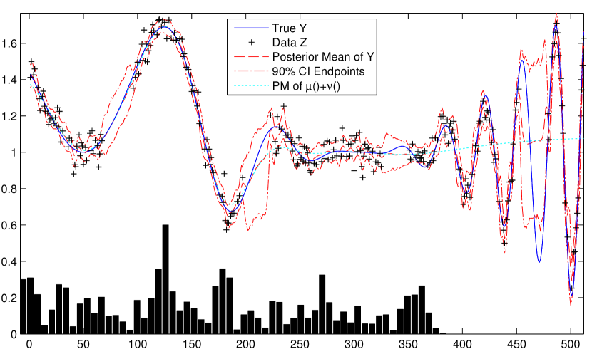
Figure 1: For Simulation Study 1, the true process $Y(\cdot)$ and one sample of the data $\mathbf{Z}$, together with the posterior mean and a point-wise posterior $90\%$ credible interval (CI) of $Y(\cdot)$, the posterior mean (PM) of $\mu(\cdot)+\nu(\cdot)$ (i.e., without $\delta(\cdot)$), and the density of the knots (histogram at the bottom) using our model

Based on this true process, we created 100 datasets of observations by adding independent normal measurement error with variance $\sigma^{2}_{\epsilon}=\hat{\sigma}^{2}_{Y}\cdot 5\%=0.004$, where $\hat{\sigma}^{2}_{Y}=0.08$ is the empirical variance of $\{Y(1),\ldots,Y(512)\}$. To examine the medium-to-long-range prediction performance of the models, we created four test intervals, in which no data was observed (collectively referred to as missing by design, or MBD). These test intervals each have length 25 and begin at locations 70, 198, 326, 454, respectively. In addition, one third of the remaining locations (henceforth referred to as missing at random, or MAR) were selected at random at each iteration of the simulation study as unobserved test locations (to test short-range prediction performance near observed locations). The remaining 275 observed locations will be denoted OBS.

To ensure comparability of the results, we assumed the measurement-error variance to be known for all models. For each of the 100 simulated datasets, each of the models was run for 10,000 MCMC iterations (thinned by a factor of 10), the first 5,000 of which were taken as burn-in (based on examination of trace plots in a pilot study). The tapering length in (9) was chosen as $L=6.5$, resulting in about 2,400 nonzero elements (less than 9 per row) for $\mathbf{V}$ in (18). The prior distributions of the parameters of the parent covariance were as described in Section 2.4, with $\mu_{\sigma}=\log(\hat{\sigma}_{Y})$ and $\mu_{\gamma}=\log(3000)$. The spatial trend, $\mu(\cdot)$ in (3), consisted only of an intercept (i.e., $\mathbf{x}(\cdot)\equiv 1$).

For the random knots, the proposal distribution for new knots (as described in step 3 of Section 3.2) was a uniform distribution on $[-9,522]$. As a pilot study using our model showed that the posterior mean of $r$ was around $11$, we used two sets of fixed knots: The first consisted of eight evenly spaced knots between locations -10 and 522, and the second set consisted of 14 evenly spaced knots between -4 and 516. For the models with nonstationary parent covariance, we took $\mathbf{b}_{\theta}(\cdot)$ in (15) to be made up of four power exponential functions with scale parameter $\lambda=74$, centered at locations 64, 192, 320, 448, respectively. One set of observations, $\mathbf{Z}$, is shown in Figure 1, together with a summary of the corresponding results using our model. Very few knots are selected between locations 380 and 500, because the process fluctuates so quickly in that area that it can basically be picked up entirely by the tapered remainder component, $\delta(\cdot)$.

To measure prediction accuracy of the models under consideration, we used the mean squared prediction error, the squared difference between the true process $Y(\cdot)$ and the posterior mean for each of the models. To quantify the accuracy of the uncertainty estimation, we also calculated the interval score, which combines the width of a credible interval (here, $95\%$ posterior credible intervals) with a penalty for not containing the true value (see Gneiting and Raftery, , 2007, Sect. 6.2). The goal is for a small interval score. Both mean squared prediction error and interval score were averaged over the 100 simulated datasets and all 512 locations (ALL), and also averaged within each of the groups of locations described earlier (OBS, MAR, MBD).

Table 2: Results of Simulation Study 1

	Random knots		8 Fixed knots		14 Fixed knots		Full model
Parent covariance	NPC	SPC	NPC	SPC	NPC	SPC	NPC	SPC
Time (min)	3.64	3.79	2.01	2.01	2.76	2.73	101.17	100.05
MSPE (ALL) $\times 100$	1.00	1.02	1.19	1.25	1.38	1.56	1.48	1.57
MSPE (OBS) $\times 100$	0.11	0.11	0.18	0.21	0.13	0.19	0.14	0.18
MSPE (MAR) $\times 100$	0.24	0.25	0.51	0.57	0.36	0.48	0.23	0.28
MSPE (MBD) $\times 100$	4.48	4.58	4.87	5.05	6.24	6.80	6.88	7.17
IS (ALL) $\times 100$	26.71	28.45	33.16	47.28	45.65	72.84	62.94	80.60
IS (OBS) $\times 100$	15.54	15.77	20.11	21.77	17.11	20.99	18.30	22.42
IS (MAR) $\times 100$	21.64	21.93	33.01	38.56	27.16	36.52	23.92	29.77
IS (MBD) $\times 100$	64.40	72.26	69.23	129.36	149.43	265.21	239.18	310.26
Posterior mean of $r$	10.59	11.24	(8)	(8)	(14)	(14)	(275)	(275 )

NPC = nonstationary parent covariance; SPC = stationary parent covariance; MSPE = mean square prediction error; IS = interval score; Time = average time for each MCMC (averaged over the 100 simulated datasets); ALL = all 512 locations; OBS = the 275 observed locations; MAR = the 137 missing-at-random locations; MBD = the 100 missing-by-design locations

The results for Simulation Study 1 are shown in Table 2. Two trends are evident in terms of both scores: Using a NPC produced better predictions than using a SPC, and random knots resulted in better predictions when compared to fixed knots. The more fixed knots were used (we even included the full model, for which $r=n$), the closer the resulting models were to their respective parent processes (which are clearly the wrong models for $Y(\cdot)$ in (23)), and the worse the scores were for the test regions (MBD).

Throughout this article, we assumed that most real-world processes do not have covariances of simple parametric form. To examine the performance of our model in the unlikely event of encountering a process that does exhibit simple parametric covariance, we conducted two more simulation studies. In Simulation Studies 2 and 3, we sampled a new true process $Y(\cdot)$ 100 times each as a constant spatial “trend” equal to 1 plus a mean-zero Gaussian process component with the Matérn covariance function of (14). For Simulation Study 2, we chose

$$\begin{split}\sigma(s)&=3\exp\big{(}\sin((1-|s/256-1|)\,2\pi)/2\big{)}\\ \gamma(s)&=600\exp\big{(}-2\sin(s\,2\pi/256)\big{)}(s/256)\\ \upsilon(s)&=3\Phi\big{(}-\sin(s\,2\pi/256)\big{)},\end{split}$$ (24)

and for Simulation Study 3, we used a stationary Matérn covariance with $\sigma(s)\equiv 3$, $\gamma(s)\equiv 600$, and $\upsilon(s)\equiv 1$. At each of the 100 iterations, we then simulated data, $\mathbf{Z}$, by adding a spatially independent measurement-error term with variance $\sigma^{2}_{\epsilon}=3^{2}\cdot 5\%=0.45$ at each observed location. The remaining setup was exactly the same as in Simulation Study 1, except that we chose $\mu_{\sigma}=\log(3)$ and $\mu_{\gamma}=\log(600)$.

Table 3: Results of Simulation Study 2

	Random knots		8 Fixed knots		14 Fixed knots
Parent covariance	NPC	SPC	NPC	SPC	NPC	SPC
Time (sec)	184.12	192.42	111.22	110.38	152.10	150.19
MSPE (ALL)	1.80	1.89	2.02	2.14	1.95	2.07
MSPE (OBS)	0.23	0.28	0.26	0.35	0.24	0.34
MSPE (MAR)	1.66	1.84	1.69	1.73	1.61	1.70
MSPE (MBD)	6.30	6.38	7.28	7.61	7.12	7.31
IS (ALL)	4.76	5.83	4.97	7.28	4.82	7.46
IS (OBS)	2.28	2.69	2.40	2.93	2.30	2.89
IS (MAR)	5.65	7.74	5.45	8.44	5.08	8.43
IS (MBD)	10.37	11.87	11.39	17.68	11.38	18.67
Posterior mean of $r$	8.82	9.78	(8)	(8)	(14)	(14)

NPC = nonstationary parent covariance; SPC = stationary parent covariance; MSPE = mean square prediction error; IS = interval score; Time = average time for each MCMC (averaged over the 100 simulated datasets); ALL = all 512 locations; OBS = the 275 observed locations; MAR = the 137 missing-at-random locations; MBD = the 100 missing-by-design locations

In Simulation Study 2 (see Table 3), the NPC models worked better than the corresponding SPC models (as expected, because the true $Y(\cdot)$ was nonstationary). Overall, random knots resulted in better predictions than fixed knots, especially for the (misspecified) SPC models.

Table 4: Results of Simulation Study 3

	Random knots		8 Fixed knots		14 Fixed knots
Parent covariance	NPC	SPC	NPC	SPC	NPC	SPC
Time (sec)	193.68	196.75	108.87	109.51	149.12	148.85
MSPE (ALL)	1.11	1.12	1.56	1.58	1.24	1.25
MSPE (OBS)	0.20	0.20	0.24	0.24	0.22	0.22
MSPE (MAR)	0.40	0.40	0.55	0.57	0.47	0.48
MSPE (MBD)	4.58	4.62	6.57	6.67	5.08	5.10
IS (ALL)	4.12	4.20	5.07	5.16	4.68	4.71
IS (OBS)	2.13	2.14	2.30	2.31	2.25	2.26
IS (MAR)	3.12	3.14	3.62	3.67	3.38	3.38
IS (MBD)	10.93	11.33	14.69	15.04	13.13	13.27
Posterior mean of $r$	10.40	10.69	(8)	(8)	(14)	(14)

NPC = nonstationary parent covariance; SPC = stationary parent covariance; MSPE = mean square prediction error; IS = interval score; Time = average time for each MCMC (averaged over the 100 simulated datasets); ALL = all 512 locations; OBS = the 275 observed locations; MAR = the 137 missing-at-random locations; MBD = the 100 missing-by-design locations

For Simulation Study 3 (see Table 4), NPC still worked slightly better than SPC, suggesting that there is no penalty in terms of predictive distributions for using the (more flexible) NPC model when the true process is stationary. The models with random knots again had the best results.

For all three simulation studies, the models with random knots resulted in longer computation times than the models with eight or 14 fixed knots.

4.2 Analysis of Soil Readings from a Gamma-Radiometer

We also compared the models of Section 4.1 using a large real-world spatial dataset. Viscarra Rossel et al., (2007) collected high-resolution soil information on Nowley farm in New South Wales, Australia. It is important to develop automated soil sensing for monitoring and precision agriculture, because conventional soil sampling is far too costly to be routinely used on a large scale.

Specifically, Viscarra Rossel et al., (2007) obtained 34,266 gamma-ray readings using a gamma-radiometer mounted on the front of a four-wheel-drive vehicle. After some preprocessing, they smoothed the data using “local kriging” and carried out a multivariate calibration of the hyperspectral gamma-ray data to predict soil properties. They showed that “kriging improved the signal-to-noise ratio of the gamma-ray spectra.” We focus here on spatial prediction of the total radioactivity count, the integrated count over the 0.4 - 2.81 mega-electronvolt spectrum, given in units of counts per second. The total count has been shown to be closely associated with the clay content in the soil (Taylor et al., , 2002; Pracilio et al., , 2004). Previously, Cressie and Kang, (2010) carried out an exploratory data analysis of total count and obtained spatial predictions using a spatial-random-effects model.

To assess prediction performance, we created a test region (called MBD) containing 409 observations. The test data were only used for model evaluation, and they were not available for model fitting. The remaining $n=33,866$ measurements, together with the test region (MBD), are shown in the top left panel of Figure 2. The spatial domain was taken to be $\mathcal{D}\colonequals(223525,225770)\times(6526400,6527930)$ in Easting and Northing.

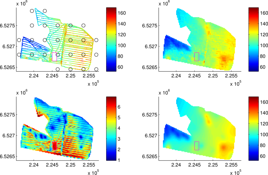
Figure 2: Top left: Gamma emissions total count observations (small colored dots) and locations of the 25 basis-function centers for $\mathbf{b}_{\theta}(\cdot)$ (black circles). Top right: Posterior mean of the true intensity using our model. Bottom left: Posterior standard deviation of the true intensity. Bottom right: Posterior mean of the smooth process without $\delta(\cdot)$ (see text). The test region (MBD) is represented by a pink rectangle. Color-scale units are counts per second; Easting and Northing are given in meters.

Following Cressie and Kang, (2010), we log-transform the (shifted) data to obtain additive measurement error:

$$Z(\mathbf{s}_{i})\colonequals\log(\textrm{TC}(\mathbf{s}_{i})+160),\;i=1,\ldots,n,$$ (25)

where TC denotes the total radioactivity count.

Cressie and Kang, (2010) identified Easting and Northing as important trend terms, and so we set $\mathbf{x}(\mathbf{s})\colonequals(1,\mathbf{s}^{\prime})^{\prime}$, where each location $\mathbf{s}\in\mathcal{D}$ is a two-dimensional vector consisting of Easting and Northing (in meters). The measurement-error variance (on the log scale) is known from another experiment to have a value of $\sigma_{\epsilon}^{2}=0.0016$ (see Cressie and Kang, , 2010). As the empirical variance of $\mathbf{Z}$ was calculated to be $\hat{\sigma}^{2}_{Z}=0.0026$ (after subtracting the trend as estimated by ordinary least squares), the signal-to-noise ratio is less than 2. Nonetheless, it is possible to distinguish signal from noise in many areas of the domain due to high sampling density (see top left panel of Figure 2).

We considered two equidistant grids of fixed knots on the domain $\mathcal{D}$, one with 64 and one with 144 locations. For the vector $\mathbf{b}_{\theta}(\cdot)$ in (15), we chose 25 power exponential functions with scale parameter 300 and centers shown in the top left panel of Figure 2. We chose a tapering length of $L=35$ in (9), which resulted in roughly 150 nonzero elements per row for $\mathbf{V}$ in (18) (i.e., about $99.56\%$ of the elements of $\mathbf{V}$ were zero). The prior distributions of the parent-covariance parameters were as described in Section 2.4, with $\mu_{\sigma}=\log(\hat{\sigma}_{Y})$ and $\mu_{\gamma}=\log(577.76)$, where $\hat{\sigma}_{Y}\colonequals\sqrt{\hat{\sigma}^{2}_{Z}-\sigma^{2}_{\epsilon}}$.

On an Intel Xeon X5560 machine with 94.5 GB RAM, we ran an MCMC for each of the models for 20,000 iterations, of which 10,000 were considered burn-in (based on examination of trace plots), and we only used every 10th of the remaining iterations for inference. We also obtained the posterior distribution of $Y(\cdot)$ at a grid of 5,707 locations. In Figure 2, using our model, we show the posterior means (top right panel) and standard deviations (bottom left panel) of the (error-free) true intensity (TI) on the original scale, defined in analogy to the transformation (25) as $\textrm{TI}(\mathbf{s})\colonequals\exp\{Y(\mathbf{s})\}-160$. We also show the posterior mean of $\exp\{\mu(\cdot)+\nu(\cdot)\}-160$ (i.e., without $\delta(\cdot)$) in the bottom right panel of Figure 2.

The model comparison was carried out on the log-scale. We obtained samples from the posterior distribution of $Z(\mathbf{s}_{j})$ at test location $\mathbf{s}_{j}$ as, $Z^{(k)}(\mathbf{s}_{j})\colonequals Y^{(k)}(\mathbf{s}_{j})+\epsilon^{(k)}(\mathbf{s}_{j})$, where the $Y^{(k)}(\mathbf{s}_{j})$ are posterior samples from $Y(\mathbf{s}_{j})$, and $\epsilon^{(k)}(\mathbf{s}_{j})\sim N(0,\sigma^{2}_{\epsilon})$ is independent “measurement error.” We then calculated the average squared distance (ASD) of the means of $\{Z^{(k)}(\mathbf{s}_{j})\}$ to the test observations $Z(\mathbf{s}_{j})$, and the interval score for $95\%$ credible intervals for $Z(\mathbf{s}_{j})$, for all models, averaged over the test locations.

Table 5: Summary of the results of the soil data analysis

	Random knots		64 Fixed knots		144 Fixed knots
Parent covariance	NPC	SPC	NPC	SPC	NPC	SPC
Time (hours)	89.87	95.05	59.02	59.15	158.84	152.36
ASD (MBD) $\times 100$	0.26	0.28	0.27	0.28	0.32	0.30
IS (MBD) $\times 100$	26.96	28.13	27.39	28.48	29.41	31.38
Posterior mean of $r$	35.57	42.88	(64)	(64)	(144)	(144)

NPC = nonstationary parent covariance; SPC = stationary parent covariance; ASD = average squared distance; IS = interval score; Time = total time for the MCMC; MBD = missing-by-design (test region)

The results are shown in Table 5. Random knots resulted in lower average squared distance and interval score than fixed knots. With the exception of average squared distance for the models with 144 fixed knots, NPC also improved over SPC. More knots resulted in less accurate predictive distributions.

Based on examination of trace plots, mixing was somewhat slower for random knots than for fixed knots and slower for NPC than for SPC (both for the soil data here and for the simulated data in Section 4.1). Because the same number of MCMC iterations was used for all models, the computation times given in Tables 2–5 can be slightly misleading. However, since the focus in this article is not parameter estimation but on prediction, and predictive performance of the models was also assessed based on an equal number of MCMC iterations, we feel that the comparison is fair.

5 Conclusions

In this article, our starting point was the Sang and Huang, (2012) approach to analyzing large spatial datasets, which combines a low-rank predictive-process component with a tapered remainder component. To achieve enough flexibility for the nonstationary processes often encountered in real-world applications, we extended this model in two ways: First, the components in the model are parameterized based on a nonstationary Matérn parent covariance function, in which the parameters vary spatially according to linear combinations of spatial basis functions. Second, for the low-rank component, which can be written as a linear combination of spatial basis functions, we make inference on the number, locations, and shapes of the basis functions. Posterior inference via reversible jump MCMC and related issues are described in detail.

The results of a simulation study (Section 4.1) and an analysis of a very large soil dataset (Section 4.2) indicate that the two extensions described above can result in improved predictive distributions, especially in terms of quantifying prediction uncertainty. We show that for (typically nonstationary) real-world processes, it should often not be the goal to approximate a simple covariance model (e.g., the stationary Matérn covariance) as closely as possible. Results indicate that our model is sufficiently flexible to overcome a misspecified parent covariance, and its flexibility does not seem to result in a penalty in the unlikely event that the truth is, in fact, a simple stationary covariance (see Simulation Study 3 in Section 4.1). Due to its adaptability, our model can be used to model highly nonstationary processes with varying levels of smoothness.

References

- (1)
- Banerjee et al., (2004) Banerjee, S., Carlin, B., and Gelfand, A. E. (2004). Hierarchical modeling and analysis for spatial data. Chapman & Hall.
- Banerjee et al., (2008) Banerjee, S., Gelfand, A. E., Finley, A. O., and Sang, H. (2008). Gaussian predictive process models for large spatial data sets. Journal of the Royal Statistical Society, Series B, 70(4):825–848.
- Berliner et al., (2000) Berliner, L. M., Wikle, C. K., and Cressie, N. (2000). Long-lead prediction of Pacific SSTs via Bayesian dynamic modeling. Journal of Climate, 13(22):3953–3968.
- Bevilacqua et al., (2012) Bevilacqua, M., Gaetan, C., Mateu, J., and Porcu, E. (2012). Estimating space and space-time covariance functions for large data sets: a weighted composite likelihood approach. Journal of the American Statistical Association, 107(497):268–280.
- Calder, (2007) Calder, C. A. (2007). Dynamic factor process convolution models for multivariate space-time data with application to air quality assessment. Environmental and Ecological Statistics, 14(3):229–247.
- Cressie, (1993) Cressie, N. (1993). Statistics for Spatial Data, revised edition. John Wiley & Sons, New York, NY.
- Cressie and Johannesson, (2006) Cressie, N. and Johannesson, G. (2006). Spatial prediction of massive datasets. In Mastering the Data Explosion in the Earth and Environmental Sciences: Proceedings of the Australian Academy of Science Elizabeth and Frederick White Conference, Canberra, Australia. Australian Academy of Science.
- Cressie and Johannesson, (2008) Cressie, N. and Johannesson, G. (2008). Fixed rank kriging for very large spatial data sets. Journal of the Royal Statistical Society, Series B, 70(1):209–226.
- Cressie and Kang, (2010) Cressie, N. and Kang, E. L. (2010). High-resolution digital soil mapping: Kriging for very large datasets. In Viscarra-Rossel, R., McBratney, A., and Minasny, B., editors, Proximal Soil Sensing, chapter 4, pages 49–63. Springer, Dordrecht, NL.
- Cressie et al., (2010) Cressie, N., Shi, T., and Kang, E. L. (2010). Fixed rank filtering for spatio-temporal data. Journal of Computational and Graphical Statistics, 19(3):724–745.
- Curriero and Lele, (1999) Curriero, F. and Lele, S. (1999). A composite likelihood approach to semivariogram estimation. Journal of Agricultural, Biological, and Environmental Statistics, 4(1):9–28.
- Eidsvik et al., (2012) Eidsvik, J., Shaby, B. A., Reich, B. J., Wheeler, M., and Niemi, J. (2012). Estimation and prediction in spatial models with block composite likelihoods using parallel computing. Submitted.
- Finley et al., (2009) Finley, A. O., Sang, H., Banerjee, S., and Gelfand, A. E. (2009). Improving the performance of predictive process modeling for large datasets. Computational Statistics & Data Analysis, 53(8):2873–2884.
- Furrer et al., (2006) Furrer, R., Genton, M. G., and Nychka, D. W. (2006). Covariance tapering for interpolation of large spatial datasets. Journal of Computational and Graphical Statistics, 15(3):502–523.
- Geman and Geman, (1984) Geman, S. and Geman, D. (1984). Stochastic relaxation, Gibbs distributions, and the Bayesian restoration of images. IEEE Transactions on Pattern Analysis and Machine Intelligence, 6(6):721–741.
- Gilbert et al., (1992) Gilbert, J. R., Moler, C., and Schreiber, R. (1992). Sparse Matrices in MATLAB: Design and Implementation. SIAM Journal on Matrix Analysis and Applications, 13(1):333–356.
- Gneiting, (2002) Gneiting, T. (2002). Compactly supported correlation functions. Journal of Multivariate Analysis, 83(2):493–508.
- Gneiting and Raftery, (2007) Gneiting, T. and Raftery, A. E. (2007). Strictly proper scoring rules, prediction, and estimation. Journal of the American Statistical Association, 102(477):359–378.
- Green, (1995) Green, P. J. (1995). Reversible jump Markov chain Monte Carlo computation Bayesian model determination. Biometrika, 82(4):711.
- Guhaniyogi et al., (2011) Guhaniyogi, R., Finley, A. O., Banerjee, S., and Gelfand, A. E. (2011). Adaptive Gaussian predictive process models for large spatial datasets. Environmetrics, 22(8):997–1007.
- Haario et al., (2001) Haario, H., Saksman, E., and Tamminen, J. (2001). An adaptive Metropolis algorithm. Bernoulli, 7(2):223–242.
- Hastings, (1970) Hastings, W. (1970). Monte Carlo sampling methods using Markov chains and their applications. Biometrika, 57(1):97–109.
- Henderson and Searle, (1981) Henderson, H. and Searle, S. (1981). On deriving the inverse of a sum of matrices. SIAM Review, 23(1):53–60.
- Higdon, (1998) Higdon, D. (1998). A process-convolution approach to modelling temperatures in the North Atlantic Ocean. Environmental and Ecological Statistics, 5(2):173–190.
- Holmes and Mallick, (2001) Holmes, C. and Mallick, B. (2001). Bayesian regression with multivariate linear splines. Journal of the Royal Statistical Society: Series B, 63(1):3–17.
- Holmes and Mallick, (2000) Holmes, C. and Mallick, B. K. (2000). Bayesian wavelet networks for nonparametric regression. IEEE Transactions on Neural Networks, 11(1):27–35.
- Kang and Cressie, (2011) Kang, E. L. and Cressie, N. (2011). Bayesian inference for the spatial random effects model. Journal of the American Statistical Association, 106(495):972–983.
- Kang et al., (2009) Kang, E. L., Liu, D., and Cressie, N. (2009). Statistical analysis of small-area data based on independence, spatial, non-hierarchical, and hierarchical models. Computational Statistics & Data Analysis, 53(8):3016–3032.
- Kanter, (1997) Kanter, M. (1997). Unimodal spectral windows. Statistics & Probability Letters, 34(4):403–411.
- Kass and Raftery, (1995) Kass, R. and Raftery, A. (1995). Bayes factors. Journal of the American Statistical Association, 90(430):773–795.
- Katzfuss, (2011) Katzfuss, M. (2011). Hierarchical Spatial and Spatio-Temporal Modeling of Massive Datasets, with Application to Global Mapping of CO. PhD Dissertation, The Ohio State University.
- Katzfuss and Cressie, (2011) Katzfuss, M. and Cressie, N. (2011). Spatio-temporal smoothing and EM estimation for massive remote-sensing data sets. Journal of Time Series Analysis, 32(4):430–446.
- Katzfuss and Cressie, (2012) Katzfuss, M. and Cressie, N. (2012). Bayesian hierarchical spatio-temporal smoothing for very large datasets. Environmetrics, 23(1):94–107.
- Kaufman et al., (2008) Kaufman, C., Schervish, M., and Nychka, D. W. (2008). Covariance tapering for likelihood-based estimation in large spatial data sets. Journal of the American Statistical Association, 103(484):1545–1555.
- Knuth, (2005) Knuth, K. (2005). Informed source separation: A Bayesian tutorial. In Sanjur, B., Cetin, E., Tekalp, E., and Kuruoglu, E., editors, European Signal Processing Conference, Antalya, Turkey.
- Lemos and Sansó, (2009) Lemos, R. T. and Sansó, B. (2009). A spatio-temporal model for mean, anomaly, and trend fields of North Atlantic sea surface temperature. Journal of the American Statistical Association, 104(485):5–18.
- Lindgren et al., (2011) Lindgren, F., Rue, H., and Lindström, J. (2011). An explicit link between Gaussian fields and Gaussian Markov random fields: the stochastic partial differential equation approach. Journal of the Royal Statistical Society, Series B, 73(4):423–498.
- Lindsay, (1988) Lindsay, B. (1988). Composite likelihood methods. In Prabhu, N. U., editor, Statistical Inference from Stochastic Processes, pages 221–239, Providence, RI. American Mathematical Society.
- Lopes et al., (2008) Lopes, H. F., Salazar, E., and Gamerman, D. (2008). Spatial dynamic factor analysis. Bayesian Analysis, 3(4):759–792.
- Mardia et al., (1998) Mardia, K., Goodall, C., Redfern, E., and Alonso, F. (1998). The kriged Kalman filter. Test, 7(2):217–282.
- Metropolis et al., (1953) Metropolis, N., Rosenbluth, A., Rosenbluth, M., Teller, A., and Teller, E. (1953). Equation of state calculations by fast computing machines. Journal of Chemical Physics, 21(6):1087–1092.
- Paciorek and Schervish, (2006) Paciorek, C. and Schervish, M. (2006). Spatial modelling using a new class of nonstationary covariance functions. Environmetrics, 17(5):483–506.
- Pracilio et al., (2004) Pracilio, G., Smettem, K., and Harper, R. (2004). New soil survey technologies to map landscape properties relevant to perennial plant performance. In Ridley, A., Feikama, P., Bennet, S., Rogers, M.-J., Wilkinson, R., and Hirth, J., editors, Salinity Solutions, Working with Science and Society, Bendigo, Victoria, Austalia. Proceedings of the Salinity Solutions Conference.
- Sang and Huang, (2012) Sang, H. and Huang, J. Z. (2012). A full scale approximation of covariance functions. Journal of the Royal Statistical Society, Series B, 74(1):111–132.
- Sang et al., (2011) Sang, H., Jun, M., and Huang, J. Z. (2011). Covariance approximation for large multivariate spatial datasets with an application to multiple climate model errors. Annals of Applied Statistics, 5(4):2519–2548.
- Shaby and Ruppert, (2012) Shaby, B. and Ruppert, D. (2012). Tapered Covariance: Bayesian Estimation and Asymptotics. Journal of Computational and Graphical Statistics, 21(2):433–452.
- Sherman and Morrison, (1950) Sherman, J. and Morrison, W. (1950). Adjustment of an inverse matrix corresponding to a change in one element of a given matrix. Annals of Mathematical Statistics, 21(1):124–127.
- Shi and Cressie, (2007) Shi, T. and Cressie, N. (2007). Global statistical analysis of MISR aerosol data: A massive data product from NASA’s Terra satellite. Environmetrics, 18:665–680.
- Stein, (1999) Stein, M. L. (1999). Interpolation of Spatial Data: Some Theory for Kriging. Springer, New York, NY.
- Stein, (2005) Stein, M. L. (2005). Nonstationary spatial covariance functions. Technical Report No. 21, Center for Integrating Statistical and Environmental Science, The University of Chicago.
- Stein, (2008) Stein, M. L. (2008). A modeling approach for large spatial datasets. Journal of the Korean Statistical Society, 37(1):3–10.
- Sun et al., (2011) Sun, Y., Li, B., and Genton, M. G. (2011). Geostatistics for large datasets. In Montero, J., Porcu, E., and Schlather, M., editors, Space-Time Processes and Challenges Related to Environmental Problems: Proceedings of the Spring School ”Advances And Challenges In Space-time Modelling Of Natural Events”. Springer.
- Taylor et al., (2002) Taylor, M., Smettem, K., Pracilio, G., and Verboom, W. (2002). Relationships between soil properties and high-resolution radiometrics, central eastern Wheatbelt, Western Australia. Exploration Geophysics, 33(2):95–102.
- van Dyk and Park, (2008) van Dyk, D. A. and Park, T. (2008). Partially collapsed Gibbs samplers: Theory and methods. Journal of the American Statistical Association, 103:790–796.
- Viscarra Rossel et al., (2007) Viscarra Rossel, R., Taylor, H. J., and McBratney, A. (2007). Multivariate calibration of hyperspectral -ray energy spectra for proximal soil sensing. European Journal of Soil Science, 58(1):343–353.
- Wikle, (2010) Wikle, C. K. (2010). Low-rank representations for spatial processes. In Gelfand, A. E., Fuentes, M., Guttorp, P., and Diggle, P., editors, Handbook of Spatial Statistics, pages 107 – 118, Boca Raton, FL. Chapman and Hall/CRC.
- Wikle and Cressie, (1999) Wikle, C. K. and Cressie, N. (1999). A dimension-reduced approach to space-time Kalman filtering. Biometrika, 86(4):815–829.
- Wikle et al., (2001) Wikle, C. K., Milliff, R., Nychka, D. W., and Berliner, L. M. (2001). Spatiotemporal hierarchical Bayesian modeling: Tropical ocean surface winds. Journal of the American Statistical Association, 96(454):382–397.
- Woodbury, (1950) Woodbury, M. (1950). Inverting modified matrices. Memorandum Report 42, Statistical Research Group, Princeton University.
- Xu et al., (2005) Xu, B., Wikle, C. K., and Fox, N. (2005). A kernel-based spatio-temporal dynamical model for nowcasting radar precipitation. Journal of the American Statistical Association, 100(472):1133–1144.