Discriminative variable selection for clustering
with the sparse Fisher-EM algorithm

Abstract

The interest in variable selection for clustering has increased recently due to the growing need in clustering high-dimensional data. Variable selection allows in particular to ease both the clustering and the interpretation of the results. Existing approaches have demonstrated the efficiency of variable selection for clustering but turn out to be either very time consuming or not sparse enough in high-dimensional spaces. This work proposes to perform a selection of the discriminative variables by introducing sparsity in the loading matrix of the Fisher-EM algorithm. This clustering method has been recently proposed for the simultaneous visualization and clustering of high-dimensional data. It is based on a latent mixture model which fits the data into a low-dimensional discriminative subspace. Three different approaches are proposed in this work to introduce sparsity in the orientation matrix of the discriminative subspace through $\ell_{1}$-type penalizations. Experimental comparisons with existing approaches on simulated and real-world data sets demonstrate the interest of the proposed methodology. An application to the segmentation of hyperspectral images of the planet Mars is also presented.

^∗ Laboratoire SAMM, EA 4543
Université Paris 1 Panthéon-Sorbonne

^† Equipe Modal’X, EA 3454
Université Paris Ouest Nanterre

1 Introduction

With the exponential growth of measurement capacities, the observed data are nowadays frequently high-dimensional and clustering such data remains a challenging problem. In particular, when considering the mixture model context, the corresponding clustering methods show a disappointing behavior in high-dimensional spaces. They suffer from the well-known curse of dimensionality [3] which is mainly due to the fact that model-based clustering methods are dramatically over-parametrized in high-dimensional spaces. Moreover, even though we dispose of many variables to describe the studied phenomenon, most of the time, only a small subset of these original variables are in fact relevant.

Several recent works have been interested to simultaneously cluster data and reduce their dimensionality by selecting relevant variables for the clustering task. A common assumption to these works is that the true underlying clusters are assumed to differ only with respect to some of the original features. The clustering task aims therefore to group the data on a subset of relevant features. This presents two practical advantages: clustering results should be improved by the removing of non informative features and the interpretation of the obtained clusters should be eased by the meaning of retained variables. In the literature, variable selection for clustering is handled in two different ways.

On the one hand, some authors such as [19, 20, 21, 29] tackle the problem of variable selection for model-based clustering within a Bayesian framework. In particular, the determination of the role of each variable is recast as a model selection problem. A first framework was proposed by Raftery and Dean [29] in which two kinds of subsets of variables are defined: a subset of relevant variables and a subset of irrelevant variables which are independent from the clustering but which can be explained from the relevant variables through a linear regression. An extension of the previous work has then been proposed by Maugis et al. [21] who consider two kinds of irrelevant variables: the ones which can be explained by a linear regression from a subset of the clustering variables and finally a set of irrelevant variables which are totally independent of all the relevant variables. The models in competition are afterward compared with the integrated log-likelihood via a BIC approximation. Even though these approaches present good results in most practical situations, their computational times are nevertheless very high and can lead to an intractable procedure in the case of high-dimensional data.

On the other hand, penalized clustering criteria have also been proposed to deal with the problem of variable selection in clustering. In the Gaussian mixture model context, several works, such as [27, 32, 35, 39] in particular, introduced a penalty term in the log-likelihood function in order to yield sparsity in the features. The penalty function can take different forms according to the constraints imposed on the structure of the covariance matrices. The introduction of a penalty term in the log-likelihood function was also used in the mixture of factor analyzers approaches, such as in [16, 36]. More recently, Witten and Tibshirani [33] proposed a general non-probabilistic framework for variable selection in clustering, based on a general penalized criterion, which governs both variable selection and clustering. It appears nevertheless that the results of such procedures are usually not sparse enough and select a large number of the original variables, especially in the case of high-dimensional data.

Other approaches focus on simultaneously clustering the data and reducing their dimensionality by feature extraction rather than feature selection. We can cite in particular, the subspace clustering methods [9, 17, 24, 23, 26, 37] which are based on probabilistic frameworks and model each group in a specific and low-dimensional subspace. Even though these methods are very efficient in practice, they present nevertheless several limitations regarding the understanding and the interpretation of the clusters. Indeed, in most of subspace clustering approaches, each group is modeled in its specific subspace which makes difficult a global visualization of the clustered data. Even though some approaches [2, 26] model the data in a common and low-dimensional subspace, they choose the projection matrix such as the variance of the projected data is maximum and this can not be sufficient to catch discriminative information about the group structure.

To overcome these limitations, Bouveyron and Brunet [6] recently proposed a new statistical framework which aims to simultaneously cluster the data and produce a low-dimensional and discriminative representation of the clustered data. The resulting clustering method, named the Fisher-EM algorithm, clusters the data into a common latent subspace of low dimensionality which best discriminates the groups according to the current fuzzy partition of the data. It is based on an EM procedure from which an additional step, named F-step, is introduced to estimate the projection matrix whose columns span the discriminative latent space. This projection matrix is estimated at each iteration by maximizing a constrained Fisher’s criterion conditionally to the current soft partition of the data. As reported in [6], the Fisher-EM algorithm turned out to outperform most of the existing clustering methods while providing a useful visualization of the clustered data. However, the discriminative latent space is defined by “latent variables” which are linear combinations of the original variables. As a consequence, the interpretation of the resulting clusters according to the original variables is usually difficult. An intuitive way to avoid such a limitation would be to keep only large loadings variables, by thresholding for instance. Even though this approach is commonly used in practice, it has been particularly criticized by Cadima [10] since it induces some misleading information. Furthermore, it often happens when dealing with high-dimensional data that a large number of noisy or non-informative variables are present in the set of the original variables. Since the latent variables are defined by a linear combination of the original ones, the noisy variables may remain in the loadings of the projection matrix and this may produce a deterioration of the clustering results.

To overcome these shortcomings, three different approaches are proposed in this work for introducing sparsity in the Fisher-EM algorithm and thus select the discriminative variables among the set of original variables. The remainder of this document is organized as follows. Section 2 reviews the discriminative latent mixture model of [6] and the Fisher-EM algorithm which was proposed for its inference. Section 3 develops three different procedures based on $\ell_{1}$ penalties for introducing sparsity into the Fisher-EM algorithm. The first approach looks for the best sparse approximate of the solution of the F-step of the Fisher-EM algorithm. The second one recasts the optimization problem involved of the F-step as a lasso regression-type problem. The last approach is based on a penalized singular value decomposition (SVD) of the matrix involved in the constrained Fisher criterion of the F-step. Numerical experiments are then presented in Section 4 to highlight the practical behavior of the three sparse versions of the Fisher-EM algorithm and to compare them to existing approaches. In section 5, a sparse version of the Fisher-EM algorithm is applied to the segmentation of hyperspectral images. Section 6 finally provides some concluding remarks and ideas for further works.

2 The DLM model and the Fisher-EM algorithm

In this section, we briefly review the discriminative latent mixture (DLM) model [6] and its inference algorithm, named the Fisher-EM algorithm, which models and clusters the data into a common latent subspace. Conversely to similar approaches, such as [8, 24, 25, 26, 37], this latent subspace is assumed to be discriminative and its intrinsic dimension is strictly bounded by the number of groups.

2.1 The DLM model

Figure 1: Graphical summary of the DLM${}_{[\Sigma_{k}\beta]}$ model.

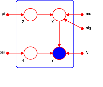
Let $\{y_{1},\dots,y_{n}\}\in\mathbb{R}^{p}$ denote a dataset of $n$ observations that one wants to cluster into $K$ homogeneous groups, i.e. adjoin to each observation $y_{i}$ a value $z_{i}\in\{1,\dots,K\}$ where $z_{i}=k$ indicates that the observation $y_{i}$ belongs to the $k$th group. On the one hand, let us assume that $\{y_{1},\dots,y_{n}\}$ are independent observed realizations of a random vector $Y\in\mathbb{R}^{p}$ and that $\{z_{1},\dots,z_{n}\}$ are also independent realizations of a random variable $Z\in\{1,\dots,K\}$. On the other hand, let $\mathbb{E}\subset\mathbb{R}^{p}$ denote a latent space assumed to be the most discriminative subspace of dimension $d\leq K-1$ such that $\mathbf{0}\in\mathbb{E}$ and $K<p$. Moreover, let $\{x_{1},\dots,x_{n}\}\in\mathbb{E}$ denote the actual data, described in the latent space $\mathbb{E}$ of dimension $d$, which are in addition presumed to be independent realizations of an unobserved random vector $X\in\mathbb{E}$. Finally, the observed variable $Y\in\mathbb{R}^{p}$ and the latent variable $X\in\mathbb{E}$ are assumed to be linked through a linear transformation:

$$Y=UX+\varepsilon,$$ (1)

where $U$ is a $p\times d$ orthonormal matrix common to the $K$ groups and satisfying $U^{t}U=\mathbf{I}_{d}$. The $p$-dimensional random vector $\varepsilon$ stands for the noise term which models the non discriminative information and which is assumed to be distributed according to a centered Gaussian density function with a covariance matrix $\Psi$ ($\varepsilon\sim\mathcal{N}(0,\Psi)$). Besides, within the latent space, $X$ is assumed, conditionally to $Z=k$, to be Gaussian :

$$X_{|Z=k}\sim\mathcal{N}(\mu_{k},\Sigma_{k})$$ (2)

where $\mu_{k}\in\mathbb{R}^{d}$ and $\mbox{$\Sigma$}_{k}\in\mathbb{R}^{d\times d}$ are respectively the mean vector and the covariance matrix of the $k$th group. Given these distribution assumptions and according to equation (1),

$$Y_{|X,Z=k}\sim\mathcal{N}(UX,\Psi),$$ (3)

and its marginal distribution is therefore a mixture of Gaussians:

$$f(y)=\sum_{k=1}^{K}\pi_{k}\phi(y;m_{k},S_{k}),$$ (4)

where $\pi_{k}$ is the mixing proportion of the $k$th group and $\phi(.;m_{k},S_{k})$ denotes the multivariate Gaussian density function parametrized by the mean vector $m_{k}=U\mu_{k}$ and the covariance matrix $S_{k}=U\Sigma_{k}U^{t}+\Psi$ of the $k$th group. Furthermore, we define the $p\times p$ matrix $W=[U,V]$ such that $W^{t}W=WW^{t}=\mathbf{I}_{p}$, where the $(p-d)\times p$ matrix $V$ is an orthogonal complement of $U$. Finally, the noise covariance matrix $\Psi$ is assumed to satisfy the conditions $V\Psi V^{t}=\beta\mathbf{I}_{p-d}$ and $U\Psi U^{t}=\mathbf{0}_{d}$, such that $\Delta_{k}=W^{t}S_{k}W$ has the following form:

$$\Delta_{k}=\left(\begin{array}[]{c@{}c}\begin{array}[]{|ccc|}\hline\cr\nobreak\leavevmode\nobreak\leavevmode\hfil&\nobreak\leavevmode\nobreak\leavevmode\hfil&\nobreak\leavevmode\nobreak\leavevmode\hfil\\ &\Sigma_{k}&\\ &&\\ \hline\cr\end{array}&\mathbf{0}\\ \mathbf{0}&\begin{array}[]{|cccc|}\hline\cr\beta&&&0\\ &\ddots&&\\ &&\ddots&\\ 0&&&\beta\\ \hline\cr\end{array}\end{array}\right)\begin{array}[]{cc}\left.\begin{array}[]{c}\\ \\ \\ \end{array}\right\}&d\leq K-1\vspace{1.5ex}\\ \left.\begin{array}[]{c}\\ \\ \\ \\ \end{array}\right\}&(p-d)\end{array}$$

These last conditions imply that the discriminative and the non-discriminative subspaces are orthogonal, which suggests in practice that all the relevant clustering information remains in the latent subspace. This model is referred to by DLM${}_{[\Sigma_{k}\beta]}$ in [6] and a graphical summary is given in Figure 1.

2.2 A family of parsimonious models

Several other models can be obtained from the DLM${}_{[\Sigma_{k}\beta]}$ model by relaxing or adding constraints on model parameters. Firstly, it is possible to consider a more general case than the DLM${}_{[\Sigma_{k}\beta]}$ by relaxing the constraint on the variance term of the non discriminative information. Assuming that $\varepsilon_{|Z=k}\sim\mathcal{N}(0,\Psi_{k})$ yields the DLM${}_{[\Sigma_{k}\beta_{k}]}$ model which can be useful in some practical cases. From this extended model, 10 parsimonious models can be obtained by constraining the parameters $\Sigma_{k}$ and $\beta_{k}$ to be common between and within the groups. For instance, the covariance matrices $\Sigma_{1},\dots,\Sigma_{K}$ in the latent space can be assumed to be common across the groups and this sub-model is referred to by $\mathrm{DLM}_{[\Sigma\beta_{k}]}$. Similarly, in each group, $\Sigma_{k}$ can be assumed to be diagonal, i.e. $\Sigma_{k}=\mathrm{diag}(\alpha_{k1},\dots,\alpha_{kd})$. This sub-model is referred to by $\mathrm{DLM}_{[\alpha_{kj}\beta_{k}]}$. These sub-models can also be declined by considering that the parameter $\beta$ is common to all classes ($\forall k,\,\beta_{k}=\beta$). A list of the $12$ different DLM models is given by Table 1 and detailed descriptions can be found in [6]. Such a family yields very parsimonious models and allows, in the same time, to fit into various situations. In particular, the complexity of the DLM${}_{[\Sigma_{k}\beta_{k}]}$ model mainly depends on the number of clusters $K$ since the dimensionality of the discriminative subspace is such that $d\leq K-1$. Notice that the complexity of the DLM${}_{[\Sigma_{k}\beta_{k}]}$ grows linearly with $p$ contrary to the traditional Gaussian models in which the complexity increases with $p^{2}$. As an illustration, if we consider the case where $p=100$, $K=4$ and $d=3$, then the number of parameters to estimate for the DLM${}_{[\Sigma_{k}\beta_{k}]}$ is $337$ which is drastically less than in the case of the Full-GMM ($20\,603$ parameters to estimate). For a comparison purpose, Table 1 presents also the complexity of other clustering methods, such as Mixt-PPCA [31], MFA [23], PGMM [24], MCFA [1] and MCUFSA [38] for which the complexity grows linearly with $p$ as well.

Model	Nb. of parameters	$K=4$ and $p=100$
$\mathrm{DLM}_{[\Sigma_{k}\beta_{k}]}$	$(K-1)+K(K-1)+(K-1)(p-K/2)+K^{2}(K-1)/2+K$	337
$\mathrm{DLM}_{[\Sigma_{k}\beta]}$	$(K-1)+K(K-1)+(K-1)(p-K/2)+K^{2}(K-1)/2+1$	334
$\mathrm{DLM}_{[\Sigma\beta_{k}]}$	$(K-1)+K(K-1)+(K-1)(p-K/2)+K(K-1)/2+K$	319
$\mathrm{DLM}_{[\Sigma\beta]}$	$(K-1)+K(K-1)+(K-1)(p-K/2)+K(K-1)/2+1$	316
$\mathrm{DLM}_{[\alpha_{kj}\beta_{k}]}$	$(K-1)+K(K-1)+(K-1)(p-K/2)+K^{2}$	325
$\mathrm{DLM}_{[\alpha_{kj}\beta]}$	$(K-1)+K(K-1)+(K-1)(p-K/2)+K(K-1)+1$	322
$\mathrm{DLM}_{[\alpha_{k}\beta_{k}]}$	$(K-1)+K(K-1)+(K-1)(p-K/2)+2K$	317
$\mathrm{DLM}_{[\alpha_{k}\beta]}$	$(K-1)+K(K-1)+(K-1)(p-K/2)+K+1$	314
$\mathrm{DLM}_{[\alpha_{j}\beta_{k}]}$	$(K-1)+K(K-1)+(K-1)(p-K/2)+(K-1)+K$	316
$\mathrm{DLM}_{[\alpha_{j}\beta]}$	$(K-1)+K(K-1)+(K-1)(p-K/2)+(K-1)+1$	313
$\mathrm{DLM}_{[\alpha\beta_{k}]}$	$(K-1)+K(K-1)+(K-1)(p-K/2)+K+1$	314
$\mathrm{DLM}_{[\alpha\beta]}$	$(K-1)+K(K-1)+(K-1)(p-K/2)+2$	311
Full-GMM	$(K-1)+Kp+Kp(p+1)/2$	20603
Com-GMM	$(K-1)+Kp+p(p+1)/2$	5453
Diag-GMM	$(K-1)+Kp+Kp$	803
Sphe-GMM	$(K-1)+Kp+K$	407
MFA	$(K-1)+Kp+Kd[p-(d-1)/2)]+Kp$	1991 ($d=3$)
Mixt-PPCA	$(K-1)+Kp+K[d(p-(d+1)/2)+d+1]+1$	1198 ($d=3$)
PGMM-CUU	$(K-1)+Kp+d[p-(d+1)/2]+Kp$	1100 ($d=3$)
MCFA	$(K-1)+Kd+p+d[p-(d+1)/2]+Kd(d+1)/2$	4330 ($d=3$)
MCUFSA	$(K-1)+Kd+1+d[p-(d+1)/2]+Kd$	3220 ($d=3$)

Table 1: Number of free parameters to estimate when $d=K-1$ for the DLM models and some classical models (see text for details).

2.3 The Fisher-EM algorithm

An estimation procedure, called the Fisher-EM algorithm, is also proposed in [6] in order to estimate both the discriminative space and the parameters of the mixture model. This algorithm is based on the EM algorithm from which an additional step is introduced, between the E and the M-step. This additional step, named F-step, aims to compute the projection matrix $U$ whose columns span the discriminative latent space. The Fisher-EM algorithm has therefore the following form, at iteration $q$:

The E-step

This step computes the posterior probabilities $t_{ik}^{(q)}$ that the observations belong to the $K$ groups using the following update formula:

$$t_{ik}^{(q)}=\hat{\pi}_{k}^{(q-1)}\phi(y_{i},\hat{\theta}_{k}^{(q-1)})/\sum_{\ell=1}^{K}\hat{\pi}_{\ell}^{(q-1)}\phi(y_{i},\hat{\theta}_{\ell}^{(q-1)}),$$ (5)

with $\hat{\theta}_{k}=\{\hat{\mu}_{k},\hat{\Sigma}_{k},\hat{\beta}_{k},\hat{U}\}$.

The F-step

This step estimates, conditionally to the posterior probabilities, the orientation matrix $U^{(q)}$ of the discriminative latent space by maximizing the Fisher’s criterion [13, 15] under orthonormality constraints:

$$\hat{U}^{(q)} = \max_{U}\quad\mathrm{trace}\left((U^{t}SU)^{-1}U^{t}S_{B}^{(q)}U\right),$$ (6)

$$\text{w.r.t.}\quad U^{t}U=\mathbf{I}_{d},$$

where $S$ stands for the covariance matrix of the whole dataset and $S_{B}^{(q)}$, defined as follows:

$$S_{B}^{(q)}=\frac{1}{n}\sum_{k=1}^{K}n_{k}^{(q)}(m_{k}^{(q)}-\bar{y})(m_{k}^{(q)}-\bar{y})^{t},$$ (7)

denotes the soft between covariance matrix with $n_{k}^{(q)}=\sum_{i=1}^{n}t_{ik}^{(q)}$, $m_{k}^{(q)}=1/n_{k}^{(q)}\sum_{i=1}^{n}t_{ik}^{(q)}y_{i}$ and $\bar{y}=1/n\sum_{i=1}^{n}y_{i}$. This optimization problem is solved in [6] using the concept of orthonormal discriminant vector developed by [14] through a Gram-Schmidt procedure. Such a process enables to fit a discriminative and low-dimensional subspace conditionally to the current soft partition of the data while providing orthonormal discriminative axes. In addition, according to the rank of the matrix $S_{B}^{(q)}$, the dimensionality of the discriminative space $d$ is strictly bounded by the number of clusters $K$.

The M-step

This third step estimates the parameters of the mixture model in the latent subspace by maximizing the conditional expectation of the complete log-likelihood:

$$Q(\theta) =-\frac{1}{2}\sum_{k=1}^{K}n_{k}^{(q)}\Bigl{[}\text{-}2\log(\pi_{k})+\mathrm{trace}(\Sigma_{k}^{-1}\hat{U}^{(q)t}C_{k}^{(q)}\hat{U}^{(q)})+\log(\left|\Sigma_{k}\right|)$$

$$\,\,\,\,\,\,\,+(p\text{-}d)\log(\beta_{k})+\frac{\mathrm{trace}(C_{k}^{(q)})\text{-}\sum_{j=1}^{d}\hat{u}_{j}^{(q)t}C_{k}^{(q)}\hat{u}_{j}^{(q)}}{\beta_{k}}+p\log(2\pi)\Bigr{]}.$$ (8)

where $C_{k}^{(q)}=\frac{1}{n_{k}^{(q)}}\sum_{i=1}^{n}t_{ik}^{(q)}(y_{i}-m_{k}^{(q)})(y_{i}-m_{k}^{(q)})^{t}$ is the empirical covariance matrix of the $k$th group and $\hat{u}_{j}^{(q)}$ is the $j$th column vector of $\hat{U}^{(q)}$, $n_{k}^{(q)}=\sum_{i=1}^{n}t_{ik}^{(q)}$. Hence, maximizing $Q$ conditionally to $\hat{U}^{(q)}$ leads to the following update formula for the mixture parameters of the model DLM${}_{[\Sigma_{k}\beta_{k}]}$:

$$\hat{\pi}_{k}^{(q)} =\frac{n_{k}^{(q)}}{n},$$ (9)

$$\hat{\mu}_{k}^{(q)} =\frac{1}{n_{k}^{(q)}}\sum_{i=1}^{n}t_{ik}^{(q)}\hat{U}^{(q)t}y_{i},$$ (10)

$$\hat{\Sigma}_{k}^{(q)} =\hat{U}^{(q)t}C_{k}\hat{U}^{(q)},$$ (11)

$$\hat{\beta}_{k}^{(q)} =\frac{\mathrm{trace}(C_{k})\text{-}\sum_{j=1}^{d}\hat{u}_{j}^{(q)t}C_{k}\hat{u}_{j}^{(q)}}{p-d}.$$ (12)

The Fisher-EM procedure iteratively updates the parameters until the Aitken criterion is satisfied (see paragraph 4.5 of [6]). The convergence properties of the Fisher-EM algorithm have been studied in [7]. It is also proposed in this work to use a stopping criterion based on the Fisher criterion involved in the F-step to improve the clustering performance. Finally, since the latent subspace has a low dimension and common to all groups, the clustered data can be easily visualized by projecting them into the estimated latent subspace.

3 Sparse versions of the Fisher-EM algorithm

Even though the Fisher-EM algorithm turns out to be efficient both for modeling and clustering data, the interpretation of clustering results regarding the original variables remains difficult. In this section, we propose therefore three different ways to introduce sparsity into the loadings of the projection matrix estimated in the F-step of the Fisher-EM algorithm.

3.1 A two-step approach

In this first approach, we propose to proceed in two steps. First, at iteration $q$, the traditional F-step of the Fisher-EM algorithm computes an estimate $\hat{U}^{(q)}$ of the orientation matrix of the discriminative latent space conditionally to the posterior probabilities $t_{ik}^{(q)}$. Then, the matrix $\hat{U}^{(q)}$ is approximated by a sparse one $\tilde{U}^{(q)}$ using the following result.

Proposition 3.1.

The best sparse approximation $\tilde{U}^{(q)}$ of $\hat{U}^{(q)}$ at the level $\lambda$ is the solution of the following penalized regression problem:

$$\min_{\mathcal{U}}\left\|X^{(q)t}-Y^{t}\mathcal{U}\right\|_{F}^{2}+\lambda\sum_{j=1}^{d}\left|\mathcal{U}_{j}\right|_{1},$$

where $\mathcal{U}=[\mathcal{U}_{1},...,\mathcal{U}_{d}]$, $\mathcal{U}_{j}\in\mathbb{R}^{p}$ is the $j$th column vector of $\mathcal{U}$, $\left\|.\right\|_{F}$ is the Frobenius norm and $X^{(q)}=\hat{U}^{(q)t}Y$.

Proof.

Let $\hat{U}^{(q)}$ be the orientation matrix of the discriminative latent space estimated by the F-step at iteration $(q)$ and let us define $X^{(q)}=\hat{U}^{(q)t}Y\,\in\mathbb{R}^{d\times n}$ the matrix of the projected data into the subspace spanned by $\hat{U}^{(q)}$, where $Y\in\mathbb{R}^{p\times n}$ denotes the original data matrix. Since $X^{(q)}$ is generated by $\hat{U}^{(q)}$, then $\hat{U}^{(q)}$ is solution of the least square regression of $X^{(q)}$ on $Y$:

$$\min_{\mathcal{U}}\left\|X^{(q)t}-Y^{t}\mathcal{U}\right\|_{F}^{2},$$

where $\mathcal{U}=[\mathcal{U}_{1},...,\mathcal{U}_{d}]$, $\mathcal{U}_{j}\in\mathbb{R}^{p}$ is the $j$th column vector of $\mathcal{U}$, $\left\|.\right\|_{F}$ is the Frobenius norm. A penalized version of this regression problem can be obtained by adding a $\ell_{1}$-penalty term as follows:

$$\min_{\mathcal{U}}\left\|X^{(q)t}-Y^{t}\mathcal{U}\right\|_{F}^{2}+\lambda\sum_{j=1}^{d}\left|\mathcal{U}_{j}\right|_{1},$$

and the solution of this penalized regression problem is therefore the best sparse approximation of $\hat{U}^{(q)}$ at the level $\lambda$.∎

The previous result allows to provide a sparse approximation $\tilde{U}^{(q)}$ of $\hat{U}^{(q)}$ but we have no guarantee that the $\tilde{U}^{(q)}$ is orthogonal as required by the DLM model. The following proposition solves this issue.

Proposition 3.2.

The best orthogonal approximation of $\tilde{U}^{(q)}$ is $\bar{U}^{(q)}=u^{(q)}v^{(q)t}$ where $u^{(q)}$ and $v^{(q)}$ are respectively the left and right singular vectors of the SVD of $\tilde{U}^{(q)}$.

Proof.

Let us consider the matrix $\tilde{U}^{(q)}$. Searching the best orthogonal approximation of the matrix $\tilde{U}^{(q)}$ is equivalent to solving the following optimization problem:

$$\min_{\mathcal{U}}\left\|\tilde{U}^{(q)}-\mathcal{U}\right\|_{F}^{2}\text{\,\,\ w.r.t. }\mathcal{U}^{t}\mathcal{U}=\mathbf{I_{d}}.$$

This problem is a nearest orthogonal Procrustes problem which can be solved by a singular value decomposition [18]. Let $u^{(q)}\Lambda^{(q)}v^{(q)t}$ be the singular value decomposition of $\tilde{U}^{(q)}$, then $u^{(q)}v^{(q)t}$ is the best orthogonal approximation of $\tilde{U}^{(q)}$. ∎

From an practical point of view, the penalized regression problem of Proposition 3.1 can be solved by alternatively regressing each column vector of the projected matrix $\hat{U}^{(q)}$. The sparse and orthogonal approximation $\bar{U}^{(q)}$ of $\tilde{U}^{(q)}$ is obtained afterward through a SVD of $\tilde{U}^{(q)}$. The following algorithm summarizes these steps.

Algorithm 1 – F-step of the sparseFEM-1 algorithm

1. At iteration $q$, compute the matrix $\hat{U}^{(q)}$ by solving (6).

2. Compute $X^{(q)}=\hat{U}^{(q)t}Y$.

3. For $j\in\{1,\dots,d\}$, solve $d$ independent penalized regression problems with the LARS algorithm [12]:

   $$\tilde{U}_{j}^{(q)}=\mathrm{arg}\min_{\mathcal{U}_{j}}\left\|x_{j}^{(q)t}-Y^{t}\mathcal{U}_{j}\right\|^{2}+\lambda\left|\mathcal{U}_{j}\right|_{1},$$

4. Repeat step 3 several times until convergence.

5. Let $\tilde{U}^{(q)}=[\tilde{U}_{1}^{(q)},...,\tilde{U}_{d}^{(q)}]$, compute the SVD of $\tilde{U}^{(q)}=u{}^{(q)}\Lambda{}^{(q)}v{}^{(q)t}$ and let $\bar{U}^{(q)}=u{}^{(q)}v{}^{(q)t}.$

Let us remark that this problem can be extended to a more general penalized regression by adding a ridge penalty term. This allows in particular to handle the $n<p$ case which occurs frequently nowadays. In such a case, the elastic-net algorithm [41] has to be used instead of the LARS algorithm in Algorithm 1.

Nevertheless, a limitation of such a procedure may be the disconnection between the estimation of the discriminative subspace and the introduction of the sparsity in the loadings of the projection matrix. To avoid that, the two following approaches aim to propose penalized Fisher criteria for which the solutions fit directly a sparse and discriminative latent subspace.

3.2 A penalized regression criterion

We therefore propose here to reformulate the constrained Fisher criterion (6) involved in the F-step of the Fisher-EM algorithm as a penalized regression problem. Consequently, the solution of this penalized regression problem will fit directly a sparse and discriminative latent subspace. To this end, let us introduce the soft matrices $H_{W}^{(q)}$ and $H_{B}^{(q)}$ which will be computed, conditionally to the E-step, at each iteration $q$ of the sparse F-step as follows:

Definition 3.1.

The soft matrices $H_{W}^{(q)}\in\mathbb{R}^{p\times n}$ and $H_{B}^{(q)}\in\mathbb{R}^{p\times K}$ are defined, conditionally to the posterior probabilities $t_{ik}^{(q)}$ computed in the E-step at iteration $q$, as follows:

$$H_{W}^{(q)} = \frac{1}{\sqrt{n}}\left[Y-\sum_{k=1}^{K}t_{1k}^{(q)}m_{k}^{(q)},\dots,Y-\sum_{k=1}^{K}t_{nk}^{(q)}m_{k}^{(q)}\right]\in\mathbb{R}^{p\times n}$$ (13)

$$H_{B}^{(q)} = \frac{1}{\sqrt{n}}\left[\sqrt{n_{1}^{(q)}}(m_{1}^{(q)}-\bar{y}),\dots,\sqrt{n_{K}^{(q)}}(m_{K}^{(q)}-\bar{y})\right]\in\mathbb{R}^{p\times K},$$ (14)

where $n_{k}^{(q)}=\sum_{i=1}^{n}t_{ik}^{(q)}$ and $m_{k}^{(q)}=\frac{1}{n}\sum_{i=1}^{n}t_{ik}^{(q)}y_{i}$ is the soft mean vector of the cluster $k$.

According to these definitions, the matrices $H_{W}^{(q)}$ and $H_{B}^{(q)}$ satisfy:

$$H_{W}^{(q)}H_{W}^{(q)t}=S_{W}^{(q)}\quad\text{and}\quad H_{B}^{(q)}H_{B}^{(q)t}=S_{B}^{(q)},$$ (15)

where $S_{W}^{(q)}=1/n\sum_{k=1}^{K}n_{k}^{(q)}C_{k}$ stands for the soft within covariance matrix computed at iteration $q$ and $S_{B}^{(q)}$ denotes the soft between covariance matrix defined in equation (7). A penalized version of the optimization problem (6) can be therefore formulated as a penalized regression-type problem:

Proposition 3.3.

The best sparse approximation $\tilde{U}^{(q)}$ of the solution of (6) at the level $\lambda$ is the solution $\hat{B}^{(q)}$ of the following penalized regression problem:

$$\min_{A,B}\sum_{k=1}^{K}\left\|R_{W}^{(q)-t}H_{B,k}^{(q)}-AB^{t}H_{B,k}^{(q)}\right\|_{F}^{2}+\rho\sum_{j=1}^{d}\beta_{j}^{t}S_{W}^{(q)}\beta_{j}+\lambda\sum_{j=1}^{d}\left|\beta_{j}\right|_{1},$$

$$\text{w.r.t. }A^{t}A=\mathbf{I}_{d},$$

where $A=[\alpha_{1},\dots,\alpha_{d}]\in\mathbb{R}^{p\times d}$, $B=[\beta_{1},\dots,\beta_{d}]\in\mathbb{R}^{p\times d}$, $R_{W}^{(q)}\in\mathbb{R}^{p\times p}$ is a upper triangular matrix resulting from the Cholesky decomposition of $S_{W}^{(q)}$, i.e. $S_{W}^{(q)}=R_{W}^{(q)t}R_{W}^{(q)}$, $H_{B,k}^{(q)}$ is the $k$th column of $H_{B}^{(q)}$ and $\rho>0$.

Proof.

First, let us consider that the matrix $A$ is fixed at iteration $q$ . Then, optimizing :

$$\min_{A,B}\sum_{k=1}^{K}\left\|R_{W}^{(q)-t}H_{B,k}^{(q)}-AB^{t}H_{B,k}^{(q)}\right\|_{F}^{2}+\rho\sum_{j=1}^{d}\beta_{j}^{t}S_{W}^{(q)}\beta_{j}$$ (16)

conditionally to $A$ leads to consider the following regularized regression problem:

$$\min_{B}\sum_{j=1}^{d}\left[\left\|H_{B}^{(q)t}R_{W}^{(q)-t}\alpha_{j}-H_{B}^{(q)t}\beta_{j}\right\|_{F}^{2}+\rho\beta_{j}^{t}S_{W}^{(q)}\beta_{j}\right],$$

with $B=[\beta_{1},\dots,\beta_{d}]$. Solving this problem is equivalent to solving $d$ independent ridge regression problem and the solution $\hat{B}^{(q)}$ is :

$$\hat{B}^{(q)}=\left(S_{B}^{(q)}+\rho S_{W}^{(q)}\right)^{-1}S_{B}^{(q)}R_{W}^{(q)-1}A.$$ (17)

By substituting $\hat{B}^{(q)}$ in Equation (16), optimizing the objective function (16) over $A$, given $A^{t}A=\mathbf{I}_{d}$ and $\hat{B}^{(q)}$ fixed, is equivalent to maximize the quantity:

$$\max_{A}\mathrm{trace}\left(\hat{B}^{(q)t}H_{B}^{(q)}H_{B}^{(q)t}R_{W}^{(q)-1}A\right),$$

$$\text{w.r.t. }A^{t}A=\mathbf{I}_{d}.$$

According to Lemma 1 of [28], this is a Procrustes problem [18] which has an analytical solution by computing the singular value decomposition of the quantity:

$$R_{W}^{(q)-t}(H_{B}^{(q)}H_{B}^{(q)t})\hat{B}^{(q)}=u^{(q)}\Lambda^{(q)}v^{(q)t},$$

where the column vectors of the $p\times d$ matrix $u^{(q)}$ are orthogonal and $v^{(q)}$ is a $d\times d$ orthogonal matrix. The solution is $\hat{A}^{(q)}=u^{(q)}v^{(q)t}$. Substituting $\hat{A}^{(q)}$ into (17) gives:

$$\hat{B}^{(q)} = R_{W}^{(q)-1}\left(R_{W}^{(q)-t}S_{B}^{(q)}R_{W}^{(q)-1}+\rho\mathbf{I}_{p}\right)^{-1}R_{W}^{(q)-t}S_{B}^{(q)}R_{W}^{(q)-1}\hat{A}^{(q)}$$

$$= R_{W}^{(q)-1}u^{(q)}\left(\Lambda^{(q)}+\rho\mathbf{I}_{p}\right)^{-1}\Lambda^{(q)}v^{(q)t}.$$

By remarking that the $d$ eigenvectors associated to the non-zero eigenvalues of the generalized eigenvalue problem (6) are the columns of $R_{W}^{(q)-1}u^{(q)},$ it follows that $\hat{B}^{(q)}$ spans the same linear subspace than the solution $\hat{U}^{(q)}$ of (6). Therefore, the solution of the penalized optimization problem:

$$\min_{A,B}\sum_{k=1}^{K}\left\|R_{W}^{(q)-t}H_{B,k}^{(q)}-AB^{t}H_{B,k}^{(q)}\right\|_{F}^{2}+\rho\sum_{j=1}^{d}\beta_{j}^{t}S_{W}^{(q)}\beta_{j}+\lambda\sum_{j=1}^{d}\left|\beta_{j}\right|_{1},$$

$$\text{w.r.t. }A^{t}A=\mathbf{I}_{d},$$

is the best sparse approximation of the solution of (6) at the level $\lambda$.∎

However and as in the previous case, the orthogonality of the column vectors of $\hat{B}^{(q)}$ is not guaranteed but this issue can be tackled by Proposition 3.2. From a practical point of view, the optimization problem of Proposition 3.3 can be solved using the algorithm proposed by [28] in the supervised case by optimizing alternatively over $B$ with $A$ fixed and over $A$ with $B$ fixed. This leads to the following algorithm in our case:

Algorithm 2 – F-step of the sparseFEM-2 algorithm

1. At iteration $q$, compute the matrices $H_{B}^{(q)}$ and $H_{W}^{(q)}$ from Equations (13) and (14). Let $S_{W}^{(q)}=H_{W}^{(q)}H_{W}^{(q)t}$ and $S_{B}^{(q)}=H_{B}^{(q)}H_{B}^{(q)t}$.

2. Compute $R_{W}^{(q)}$ by using a Cholesky decomposition of $S_{W}^{(q)}+\gamma/p\,\mathrm{trace}(S_{W}^{(q)})=R_{W}^{(q)t}R_{W}^{(q)}$.

3. Initialization:

   Let $B^{(q)}$ be the eigenvectors of $S^{-1}S_{B}^{(q)}$ .

   Compute the SVD $R_{W}^{(q)-t}S_{B}^{(q)}B^{(q)}=u^{(q)}\Lambda^{(q)}v^{(q)t}$ and let $A^{(q)}=u^{(q)}v^{(q)t}$.

4. Solve $d$ independent penalized regression problems. For $j=1,\dots,d$:

   $$\hat{\beta}_{j}^{(q)}=\mathrm{arg}\min_{\beta_{j}}\left(\beta_{j}^{t}W^{(q)t}W^{(q)}\beta_{j}-2\tilde{Y}^{(q)t}W^{(q)}\beta_{j}+\lambda_{1}\left\|\beta_{j}\right\|_{1}\right),$$

   where $W^{(q)}=\left(\begin{array}[]{c}H_{B}^{(q)t}\\ \sqrt{\rho}R_{W}^{(q)}\end{array}\right)$ and $\tilde{Y}^{(q)}=\left(\begin{array}[]{c}H_{B}^{(q)t}R_{W}^{(q)-1}\alpha_{j}^{(q)}\\ \mathbf{O}_{p}\end{array}\right)$.

5. Let $\hat{B}^{(q)}=[\hat{\beta}_{1},\dots,\hat{\beta}_{d}]$. Compute the SVD of $R_{W}^{(q)-t}S_{B}^{(q)}\hat{B}^{(q)}=u^{(q)}\Lambda^{(q)}v^{(q)t}$ and let $A^{(q)}=u^{(q)}v^{(q)t}$.

6. Compute the SVD of $\hat{B}^{(q)}=u^{\prime(q)}\Lambda^{\prime(q)}v^{\prime(q)t}$ and let $\bar{U}^{(q)}=u^{\prime(q)}v^{\prime(q)t}.$

7. Repeat steps several times until convergence.

3.3 A penalized singular value decomposition

In this last approach, we reformulate the constrained Fisher criterion (6) involved in the F-step of the Fisher-EM algorithm as a regression problem which can be solved by doing the SVD of the matrix of interest in this regression problem. A sparse approximation of the solution of this regression problem will be obtained by doing a penalized SVD [34] instead of the SVD. To that end, let us consider the following result.

Proposition 3.4.

The solution of (6) is also solution of the following constrained optimization problem:

$$\min_{\mathcal{U}}\sum_{\ell=1}^{p}\left\|S_{B,\ell}^{(q)}-\mathcal{U}\mathcal{U}^{t}S_{B,\ell}^{(q)}\right\|^{2}$$

$$\text{w.r.t. }\mathcal{U}^{t}\mathcal{U}=\mathbf{I}_{d},$$

where $S_{B,\ell}^{(q)}$ is the $\ell$th column of the soft between covariance matrix $S_{B}^{(q)}$ computed at iteration $q$.

Proof.

Let us first prove that minimizing the quantity $\sum_{\ell=1}^{p}||S_{B,\ell}^{(q)}-UU^{t}S_{B,\ell}^{(q)}||^{2}$ is equivalent to maximize $\mathrm{trace}(U^{t}S_{B}^{(q)}S_{B}^{(q)t}U)$. To that end, we can write down the following equalities:

$$\sum_{\ell=1}^{p}\left\|S_{B,\ell}^{(q)}-UU^{t}S_{B,\ell}^{(q)}\right\|^{2} = \sum_{\ell=1}^{p}\mathrm{trace}\left(S_{B,\ell}^{(q)t}(\mathbf{I}_{p}-UU^{t})^{t}(\mathbf{I}_{p}-UU^{t})S_{B,\ell}^{(q)}\right)$$

$$= \mathrm{trace}\left((\mathbf{I}_{p}-UU^{t})^{t}(\mathbf{I}_{p}-UU^{t})\sum_{\ell=1}^{p}S_{B,\ell}^{(q)}S_{B,\ell}^{(q)t}\right)$$

$$= \mathrm{trace}\left(S_{B}^{(q)t}(\mathbf{I}_{p}-UU^{t})S_{B}^{(q)}\right)$$

$$= \mathrm{trace}(S_{B}^{(q)t}S_{B}^{(q)})-\mathrm{trace}(U^{t}S_{B}^{(q)}S_{B}^{(q)t}U).$$

Consequently, minimizing over $U$ the quantity $\sum_{\ell=1}^{p}||S_{B,\ell}^{(q)}-UU^{t}S_{B,\ell}^{(q)}||^{2}$ is equivalent to maximize $\mathrm{trace}(U^{t}S_{B}^{(q)}S_{B}^{(q)t}U)$ according to $U$. Let us now consider the SVD of the $n\times p$ matrix $S_{B}^{(q)}=u\Lambda v^{t}$ where $u$ and $v$ stands for respectively the left and right singular vectors of $S_{B}^{(q)}$ and $\Lambda$ is a diagonal matrix containing its associated singular values. Since the matrix $S_{B}^{(q)}$ has a rank $d$ at most equal to $K-1<p$, with $K$ the number of clusters, then only $d$ singular values of the matrix $S_{B}^{(q)}$ are non zeros, which enables us to write $S_{B}^{(q)}=u\Lambda_{d}v^{t}$, where $\Lambda_{d}=\mathrm{diag}(\lambda_{1},\dots,\lambda_{d},0,\dots,0)$. Moreover, by letting $U=u_{d}$ the $d$ first left eigenvectors of $S_{B}$, then:

$$\mathrm{trace}\left(U^{t}S_{B}S_{B}^{t}U\right) = \mathrm{trace}\left(U^{t}(u\Lambda_{d}v^{t})(u\Lambda_{d}v^{t})^{t}U\right),$$

$$= \mathrm{trace}\left(U^{t}u\Lambda_{d}\Lambda_{d}^{t}u^{t}U\right),$$

$$= \sum_{j=1}^{d}\lambda_{j}^{2}.$$

Consequently, the $p\times d$ orthogonal matrix $\hat{U}$ such that $\sum_{\ell=1}^{p}||S_{B,\ell}^{(q)}-UU^{t}S_{B,\ell}^{(q)}||^{2}$ is minimized, is the matrix made of the $d$ first left eigenvectors of $S_{B}^{(q)}$. Besides, since $S_{B}^{(q)}$ is symmetric and semi-definite positive, the matrix $\hat{U}$ contains also the eigenvectors associated with the $d$ largest eigenvalues of $S_{B}^{(q)2}$ and therefore the ones of $S_{B}^{(q)}$. Therefore, assuming without loss of generality that $S=\mathbf{I}_{p}$, $\hat{U}$ is also solution of the constrained optimization problem (6) involved in the original F-step. ∎

The optimization problem of Proposition (3.4) can be seen as looking for the projection matrix $\mathcal{U}$ such that the back-projection $\mathcal{U}\mathcal{U}^{t}S_{B,\ell}^{(q)}$ is as close as possible to $S_{B,\ell}^{(q)}$. In [34], Witten et al. have considered such a problem with a constraint of sparsity on $\mathcal{U}$. To solve this problem, they proposed an algorithm which performs a penalized SVD of the matrix of interest in the constrained optimization problem. Therefore, it is possible to obtain a sparse approximation $\tilde{U}^{(q)}$ of the solution of (6) by doing a penalized SVD of $S_{B}^{(q)}$ with the algorithm of [34]. As previously, the orthogonality of the column vectors of $\tilde{U}^{(q)}$ is not guaranteed but this issue can be again tackled by Proposition 3.2. From a practical point of view, this third approach can be implemented as follows:

Algorithm 3 – F-step of the sparseFEM-3 algorithm

1. Let $M_{1}=S_{B}^{(q)}$ and $d=\mathrm{rank}\left(S_{B}\right).$

2. For $j\in\{1,\dots,d\}$:

   1. Solve $\hat{u}_{j}^{(q)}=\mathrm{arg}\max_{u_{j}}u_{j}^{t}M_{j}v_{j}$ w.r.t. $\left\|u_{j}\right\|_{2}^{2}\leq 1$, $\left\|v_{j}\right\|_{2}^{2}\leq 1$ and $\sum_{\ell=1}^{p}\left|u_{j\ell}^{(q)}\right|\leq\lambda_{1}$ using the penalized SVD algorithm of [34].

   2. Update $M_{j+1}=M_{j}-\lambda_{j}u_{j}^{(q)}v_{j}^{t}$.

3. $\hat{U}^{(q)}=[\hat{u}_{1}^{(q)},\dots,\hat{u}_{d}^{(q)}]$.

4. Compute the SVD of $\hat{U}^{(q)}=u^{(q)}\Lambda^{(q)}v^{(q)t}$ and let $\tilde{U}^{(q)}=u^{(q)}v^{(q)t}$.

3.4 Practical aspects

The introduction of sparsity in the Fisher-EM algorithm presents several practical aspects among which the ability to interpret the discriminative axes. However, two questions remain: the choice of the hyper-parameter which determines the level of sparsity and the implementation strategy in the Fisher-EM algorithm. Both aspects are discussed below.

Choice of the tuning parameter

The choice of the threshold $\lambda$ is an important problem since the number of zeros in the $d$ discriminative axes depends directly on the degree of sparsity. In [40], Zou et al. chose the hyper-parameter of their sparse PCA with a criterion based on the explanation of the variance approximated by the sparse principal components. In [33], Witten and Tibshirani proposed for their sparse-kmeans to base the choice of the tuning parameter on a permutation method closely related to the gap statistic previously proposed by Tibshirani et al. [30] for estimating the number of components in standard kmeans. Since our model is defined in a Gaussian mixture context, we propose to use the BIC criterion to select the threshold $\lambda$. According to the consistency results obtained by Zou et al. [42] and the fact that the sparsity constraint is applied on the projection matrix $U$, the effective number of parameters to estimate in the DLM${}_{[\Sigma_{k}\beta_{k}]}$ model is:

$$\gamma_{e}=(K-1)+Kd+\left(d[p\text{−}(d+1)/2]-\mathbf{d_{e}}\right)+Kd(d+1)/2+K$$

where $\mathbf{d_{e}}$ is the number of zeros in the loading matrix. In the same manner, this effective number of parameters to estimate can be declined for the $11$ other sub-models of the DLM family.

Implementation of the sparse Fisher-EM algorithm

We identified two different ways to implement the sparse versions of the Fisher-EM algorithm. First, it could be possible to replace the usual F-step of the Fisher-EM algorithm by a sparse F-step developed previously. The resulting algorithm would sparsify at each iteration the projection matrix $U$ before estimating the model parameters. This can however leads to some drawbacks since an early introduction of the $\ell_{1}$ penalty could penalize too much the loadings of the projection matrix, in particular if the initialization is far away from the optimal situation. An alternative implementation would be to, first, execute the traditional Fisher-EM algorithm until convergence and, then, initialize the sparse Fisher-EM algorithm with the result of the Fisher-EM algorithm. This strategy should combine the efficiency of the standard Fisher-EM algorithm with the advantage of having a sparse selection of discriminative variables. We therefore recommend this second implementation and it will be used in the experiments presented in the following sections.

4 Experimental comparison

This section presents comparisons with existing variable selection techniques on simulated and real-world data sets.

4.1 Comparison on simulated data

Simulation	Method	Clustering error	non-zero variables
$n=30$ $\mu=0.6$	kmeans	$0.48\pm 0.05$	$25.0\pm 0.0$
	sparse-kmeans	$0.47\pm 0.07$	$19.0\pm 6.6$
	Clustvarsel	$0.62\pm 0.06$	$22.2\pm 1.2$
	Selvarclust	$0.40\pm 0.03^{*}$	$8.1\pm 1.9^{*}$
	sparseFEM-1	$0.47\pm 0.06$	$2.6\pm 0.9$
	sparseFEM-2	$0.48\pm 0.07$	$4.7\pm 1.8$
	sparseFEM-3	$0.48\pm 0.03$	$2.0\pm 0.0$
$n=30$ $\mu=1.7$	kmeans	$0.14\pm 10.2$	$25.0\pm 0.0$
	sparse-kmeans	$0.08\pm 0.06$	$23.6\pm 0.8$
	Clustvarsel	$0.41\pm 0.10$	$16.6\pm 10.4$
	Selvarclust	$0.08\pm 0.08^{*}$	$6.8\pm 1.4^{*}$
	sparseFEM-1	$0.14\pm 0.13$	$3.5\pm 0.8$
	sparseFEM-2	$0.20\pm 0.12$	$5.4\pm 2.2$
	sparseFEM-3	$0.17\pm 0.11$	$2.0\pm 0.0$
$n=300$ $\mu=0.6$	kmeans	$0.43\pm 0.03$	$25.0\pm 0.0$
	sparse-kmeans	$0.46\pm 0.03$	$24.0\pm 0.5$
	Clustvarsel	$0.42\pm 0.03$	$25.0\pm 0.0$
	Selvarclust	$0.34\pm 0.02^{*}$	$7.0\pm 1.7^{\text{*}}$
	sparseFEM-1	$0.42\pm 0.03$	$2.4\pm 1.0$
	sparseFEM-2	$0.43\pm 0.03$	$5.2\pm 2.7$
	sparseFEM-3	$0.43\pm 0.04$	$2.3\pm 1.1$
$n=300$ $\mu=1.7$	kmeans	$0.05\pm 0.06$	$25.0\pm 0.0$
	sparse-kmeans	$0.05\pm 0.01$	$15.0\pm 0.0$
	Clustvarsel	$0.05\pm 0.01$	$25.0\pm 2.0$
	Selvarclust	$0.05\pm 0.01^{*}$	$5.6\pm 0.9^{*}$
	sparseFEM-1	$0.04\pm 0.01$	$10.2\pm 2.4$
	sparseFEM-2	$0.05\pm 0.01$	$8.8\pm 1.7$
	sparseFEM-3	$0.04\pm 0.01$	$5.6\pm 1.6$

Table 2: Clustering errors and numbers of non-zero variables averaged over 20 simulations for several clustering methods with $p=25$ and $q=5$. The results of Selvarclust are reported from [11].

This first experiment aims to compare on simulated data the performances of the proposed sparseFEM algorithms (sparseFEM-1, sparseFEM-2, sparseFEM-3) to several competitors: Clustvarsel of Raftery and Dean [29], Selvarclust of Maugis et al. [22] and sparse-kmeans of Witten and Tibshirani [33]. For this experiment, we replicated the simulation proposed in Section 3.3 of [33]. We simulated $K=3$ Gaussian components of $n$ observations in a $25$-dimensional observation space whose components differ only on $q=5$ features. The used parameters were $\mu_{kj}=\mu\times(\mathbf{1}_{k=1,j\leq q},-\mathbf{1}_{k=2,j\leq q}),\,\forall k\in\{1,2,3\}$ and $\forall j\in\{1,\dots,p\}$ for the mean components and $\sigma_{kj}^{2}=1$ for the variance terms. Moreover, four different situations are considered: $n=30$ or $300$ and $\mu=0.6$ or $1.7$. Each simulation was replicated $25$ times.

Table 2 presents the means and standard deviations for both the clustering error and the number of non-zero variables for kmeans, sparse-kmeans, Clustvarsel, Selvarclust and the 3 procedures of sparseFEM. Note that the results of Selvarclust corresponds to clustering errors and non-zero variable rates found in [11]. Moreover, the reported results concerning the 3 sparse Fisher-EM algorithms were obtained with the DLM${}_{[\alpha_{k}\beta]}$ model for a sparsity level corresponding to the highest BIC value obtained at each trial.

Two main remarks can be done on the results presented in Table 2. First, by considering either the most difficult clustering cases ($n=30$ and $\mu=0.6$) or the easiest one ($n=300$ and $\mu=0.6$ or $1.7$), all approaches present approximatively the same results in terms of clustering error rate. The methods differ however in the number of variables they retain to perform the clustering: Clustevarsel, sparseFEM-1, sparseFEM-2 and sparseFEM-3 turn out to select significantly less variables than sparse-kmeans and Clustvarsel. In particular, Clustevarsel and the sparseFEM algorithms select a number of useful variables consistent with the actual number of meaningful variables ($q=5$). Second, in the situation where $n=30$ and $\mu=1.7$, Selvarclust and sparse-kmeans present the lowest misclassification rate ($0.08$), even though the clustering error of sparseFEM-1 and kmeans remains relatively low ($0.14$). However, as previously, only Clustevarsel and the sparseFEM algorithms select a number of variables close to the right number of discriminative features.

4.2 Comparison on real data sets

Real-world data sets are now used to compare the efficiency of the sparseFEM algorithms to its competitors for both the clustering and variable selection tasks. We considered 7 different benchmark data sets coming mostly from the UCI machine learning repository. We selected these data sets because they represent a wide range of situations in term of number of observations $n$, number of variables $p$ and number of groups $K$. These characteristics are given in the top row of Table 4.2 and a detailed description of these data sets can be found in [6].

For this experiment, we used the 3 sparseFEM algorithms and the 3 sparse methods introduced previously (sparse-kmeans, Clustvarsel and Selvarclust). Since the evaluation of the clustering performance is a complex and very discussed problem, we chose to evaluate the clustering performance as the adequacy between the resulting partition of the data and the known labels for these data. For each data set, the sparseFEM algorithms were initialized with a common random partition drown from a multinomial distribution with equal prior probabilities. For Clustvarsel, Selvarclust and sparse-kmeans, the initialization was done with their own deterministic procedure. Moreover, for each method, the number $K$ of groups has been fixed to the actual one. For Clustvarsel, Selvarclust and sparse-kmeans, the determination of the other free parameters was done according to the tools provided by each approach. For the sparseFEM algorithms, we used the penalized BIC criterion to select the model and the level of sparsity. More precisely, we first chose the model presenting the highest average BIC value on 20 replications. Then, given the selected model, we selected the level of sparsity associated with the highest BIC value.

	iris	wine	chiro	zoo	glass	satimage	usps358
	(p=4,K=3)	(p=13,K=3)	(p=17,K=3)	(p=16,K=7)	(p=9,K=7)	(p=36,K=6)	(p=256,K=3)
Approaches	(n=150)	(n=178)	(n=178)	(n=101)	(n=214)	(n=4435)	(n=1726)
sparseFEM-1	96.5$\pm 0.3$	97.8$\pm 0.2$	84.2$\pm 11$	71.4$\pm 8.5$	50.2$\pm 1.9$	69.6$\pm 0.1$	84.7$\pm 3.2$
	(2.0$\pm 0.0$)	(2.0$\pm 0.0$)	(2.3$\pm 0.5$)	(13$\pm 2.5$)	(6.0$\pm 1.0$)	(36$\pm 0.0$)	(5.5$\pm 0.7$)
sparseFEM-2	89.9$\pm 0.4$	98.3$\pm 0.0$	84.8$\pm 12$	70.1$\pm 12.2$	48.4$\pm 3.0$	67.5$\pm 1.6$	82.8$\pm 9.1$
	(4.0$\pm 0.0$)	(4.0$\pm 0.0$)	(2.0$\pm 0.6$)	(14$\pm 3.6$)	(6.6$\pm 0.7$)	(36$\pm.0.0$)	(15.5$\pm 16$)
sparseFEM-3	96.5$\pm 0.3$	97.8$\pm 0.0$	82.9$\pm 12$	72.0$\pm 4.3$	48.2$\pm 2.7$	71.8$\pm 2.3$	79.1$\pm 7.4$
	(2.0$\pm 0.3$)	(2.0$\pm 0.0$)	(2.0$\pm 0.0$)	(10$\pm 2.8$)	(7.0$\pm 0.0$)	(36$\pm 0.0$)	(6.0$\pm 1.3$)
sparse-kmeans	90.7	94.9	95.3	79.2	52.3	71.4	74.7
	(4.0)	(13.0)	(17.0)	(16.0)	(6.0)	(36.0)	(213)
Clustvarsel	96.0	92.7	71.1	75.2	48.6	58.7	48.3
	(3.0)	(5.0)	(6.0)	(3.0)	(3.0)	(19.0)	(6.0)
Selvarclust	96.0	94.4	92.6	92.1	43.0	56.4	36.7
	(3.0)	(5.0)	(8.0)	(5.0)	(6.0)	(22.0)	(5.0)

Clustering accuracies and their standard deviations (in percentage) on 7 UCI datasets (iris, wine, chironomus, zoo, glass, satimage, usps358) averaged on 20 trials. The average number of nonzero variables is reported in brackets. No standard deviation is reported for Clustvarsel/Selvarclust and sparse-kmeans since their initialization procedure is deterministic and always provides the same initial partition.

Table 4.2 presents the average clustering accuracies and the associated standard deviations obtained for the 6 approaches. The average number of non-zero variables is also reported within brackets in the table. The results associated to the sparseFEM algorithms have been obtained by averaging over $20$ trials with random initializations. The lack of standard deviations for Clustvarsel, Selvarclust and sparse-kmeans is due to the deterministic initializations they use. It first appears that the three sparse versions of the Fisher-EM algorithm perform rather similarly both in term of clustering and variable selection. It also appears clearly that the sparseFEM algorithms are competitive to existing methods regarding both the clustering performances and the selection of variables. Indeed, the sparseFEM algorithms obtain the best clustering accuracies on 4 of the 7 data sets whereas sparse-kmeans and Selvarclust obtain the best clustering accuracies on respectively 2 and 1 data sets. The sparseFEM algorithms differ also from sparse-kmeans regarding the number of variables retained to perform the clustering. Indeed, sparse-kmeans turns out to frequently select a large number of variables whereas sparseFEM is usually rather sparse in the number of selected variables. Finally, Clustvarsel and Selvarclust turn out to select most of the time few variables, particularly in high-dimensional spaces, which seems to obstruct their clustering performance. To summarize, this experiment has shown that the sparseFEM algorithms seem to be good compromises between sparse-kmeans and Clustvarsel /Selvarclust in term of variable selection and, certainly thanks to this characteristic, they also provide good clustering results.

4.3 Comparison on the usps358 data set

We focus now on the usps358 dataset to stress the role of variable selection in the interpretation of clustering results. The original dataset is made of $7\,291$ images divided in 10 classes corresponding to the digits from 0 to 9. Each digit is a $16\times 16$ gray level image represented as a 256-dimensional vector. For this experiment, we extracted a subset of the data ($n=1\,756$) corresponding to the digits 3, 5 and 8 which are the three most difficult digits to discriminate. This smaller dataset is hereafter called usps358. Figure 4 depicts the group mean images obtained from the true labels in the usps358 dataset. For this experiment, we used the three sparseFEM algorithms with the model and the level of sparsity selected in the previous experiment for this data set. For Clustvarsel, Selvarclust and sparse-kmeans, the level of sparsity was again selected with their own selection procedure.

(a)

(b)

(c)

Figure 2: Group means obtained from the true labels in the USP358 datasets.

(a) Sparse-kmeans

(b) Clustvarsel

(c) Selvarclust

Figure 3: Variable selection obtained from (a) the sparse-kmeans algorithm, (b) the Clustvarsel approach and (c) the Selvarclust approach.

(a) sparseFEM-1

(b) sparseFEM-2

(c) sparseFEM-3

Figure 4: Variable selection obtained from (a) the sparseFEM-1, (b) the sparseFEM-2 and (c) the sparseFEM-3 procedures with sparsity levels selected by the penalized BIC.

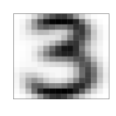
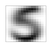
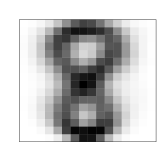
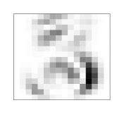
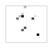
Figures 4 illustrates, as images, the features selected respectively by sparse-kmeans (Figure 4.a), Clustvarsel (Figure 4.b) and Selvarclust (Figure 4.c). In Figure 4.a, the weight assigned by sparse-kmeans to each feature is represented by gray levels: lighter is the pixel, weaker is the absolute value of the weight of the associated feature. For Clustvarsel and Selvarclust, only the selected variables are depicted and are associated to black pixels as it is illustrated in Figures 4.b and 4.c respectively. These representations are associated to the following clustering accuracies $74.7\%$, $48.3\%$ and $36.7\%$ for sparse-kmeans, Clustvarsel and Selvarclust respectively. For the 3 sparseFEM algorithms, we superimposed in a same figure the absolute values of the loadings of the two discriminative axes fitted by the sparseFEM-1, sparseFEM-2 and sparseFEM-3 procedures. The associated clustering accuracies are respectively $84.7\%$, $82.8\%$ and $79.1\%$.

First of all, it appears that Clustvarsel and Selvarclust select significantly fewer variables than both sparse-kmeans or the sparseFEM procedures. Furthermore, most of the selected variables by Clustvarsel and Selvarclust turn out to be irrelevant to discriminate the digit 3 from the digits 5 and 8. For instance, in Figures 4.b and 4.c, we can observe that the black pixels located in right bottom corner, do not correspond to any discriminative variable. This certainly explain the poor clustering performances ($48.3\%$ for Clustvarsel and $36.7\%$ for Selvarclust) observed on this data set for these methods. On the contrary, sparse-kmeans turns out to perform well in term of clustering performance ($74.7\%$ of clustering accuracy). Nevertheless, the number of selected variables remains higher (213 selected variables amongst 256 original ones) than we would expect to ease the interpretation of results. Finally, sparseFEM-1 and sparseFEM-2 seem to answer quite well to both the clustering task and the task of feature selection. Indeed, on the one hand, the subset of selected pixels remains small for both algorithms: 6 and 15 pixels are selected amongst 256 for sparseFEM-1 and sparseFEM-2 respectively. Furthermore, the selected pixels appear to be relevant to discriminate the classes associated with the three digits. For instance, the darker pixel on the bottom right corner of Figure 4.b discriminates the digit 8 from the digits 3 and 5. On the other hand, and certainly due to this relevant selection of variables, both algorithms perform particularly well on this high-dimensional data set ($84.7\%$ for sparseFEM-1 and $82.8\%$ for sparseFEM-2). However, on this data set, the sparseFEM-3 procedure shows a disappointing behavior regarding the variable selection even though its clustering performance remains satisfying. The fact that sparseFEM-3 succeeds in clustering the data set even with a bad selection of variables is certainly due to the nature of the DLM model which models also the non discriminative information through the parameter $\beta_{k}$.

Table 3 presents the computing time of the studied clustering methods (for a given model and with $\lambda$ and $K$ fixed) for clustering the usps358 data set. As we can remark, our procedures are much faster than the sparse-kmeans, Clustvarsel and Selvarclust algorithms. Consequently, the sparseFEM algorithms appear once again to be good compromises, in practice, to cluster high-dimensional data and select a set of discriminative variables in a reasonable time.

Approaches:	Procedure time (sec)	Approaches:	Procedure time (sec)
sparseFEM-1	$729.04$	sparse-kmeans	$1\,567.75$
sparseFEM-2	$387.12$	Clustvarsel	$2\,957.70$
sparseFEM-3	$409.61$	Selvarclust	$9\,257.10$

Table 3: Computing times for the 3 versions of the sparseFEM algorithm, sparse-kmeans, Clustvarsel and Selvarclust on the USPS358 data (for a given model and with $\lambda$ and $K$ fixed).

5 Application to the segmentation of hyperspectral images

Figure 5: Image of the studied zone of the Martian surface.

Figure 6: Some of the 38 400 measured spectra described on 256 wavelengths (see text for details).

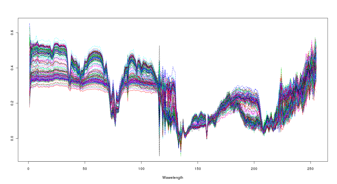
Here, we propose to use sparseFEM to segment hyperspectral images of the Martian surface. Visible and near infrared imaging spectroscopy is a key remote sensing technique to study the system of the planets. Imaging spectrometers, which are inboard of an increasing number of satellites, provide high-dimensional hyperspectral images. In March 2004, the OMEGA instrument (Mars Express, ESA) [4] has collected 310 Gbytes of raw images. The OMEGA imaging spectrometer has mapped the Martian surface with a spatial resolution varying between 300 to 3000 meters depending on the spacecraft altitude. It acquired for each resolved pixel the spectrum from 0.36 to 5.2 µm in 256 contiguous spectral channels. OMEGA is designed to characterize the composition of surface materials, discriminating between various classes of silicates, hydrated minerals, oxides and carbonates, organic frosts and ices. For this experiment, a $300\times 128$ image of the Martian surface is considered and a 256-dimensional spectral observation is therefore associated to each of the 38 400 pixels. Figure 5 presents an image of the studied zone and Figure 6 shows some of the 38 400 measured spectra. According to the experts, there are $K=5$ mineralogical classes to identify.

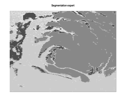
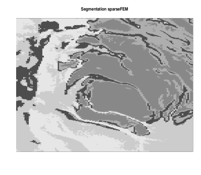
The sparseFEM-1 algorithm was applied to this dataset using the model $\mathrm{DLM}_{[\alpha_{kj}\beta]}$ and a sparsity ratio equals to $0.1$ (it refers to the ratio of the $\ell_{1}$ norm of the coefficient vector relative to the norm at the full least square solution). The sparseFEM algorithm was initialized with the results of the Fisher-EM algorithm and the whole segmentation process took 18 hours on a 2.6 Ghz computer. Figure 7 presents, on the right panel, the segmentation into $5$ mineralogical classes of the studied zone with the sparseFEM algorithm. In comparison, the left panel of Figure 7 shows the segmentation obtained by experts of the domain using a physical model. It first appears that the two segmentations agree globally on the mineralogical nature of the surface of the studied zone (60.30% of agreement). We recall that both segmentations do not exploit the spatial information. When looking at the top-right quarter of the image, we can notice that sparseFEM seems to provide a finer segmentation than the segmentation based on the physical model. Indeed, sparseFEM segments better than the physical model the fine “rivers” which can be seen on Figure 5.

Expert segmentation	SparseFEM segmentation

Figure 7: Segmentation of the hyperspectral image of the Martian surface using a physical model build by experts (left) and sparseFEM (right).

Figure 8: Mean spectra of the 5 groups formed by sparseFEM and selection of the discriminative wavelengths (indicated by gray rectangles).

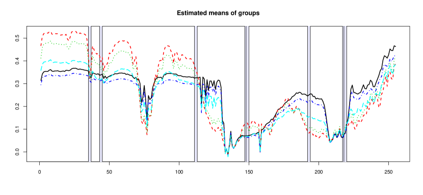
Finally, Figure 8 shows the mean spectra of the 5 groups formed by sparseFEM and the selection of the discriminative wavelengths. SparseFEM selected 8 original variables (wavelengths) as discriminative variables, i.e. the rows associated to these variables were non-zero in the loading matrix $U$. Looking closely at the selection, we indeed notice that the first selected variable (from left to right) discriminates the blue group from the others. The second selected variable discriminates the red and green groups from the black, blue and light blue groups whereas the third selected variable allows to discriminate the red, green and black groups from the blue and light blue groups. Similarly, the fourth and fifth selected variables discriminate the red and green groups from the black, blue and light blue groups whereas the sixth, seventh and eighth selected variable allows to discriminate the red, green and light blue groups from the blue and black groups.

A possible interest of such a selection could be the measurement of only a tens of wavelengths for future acquisitions instead of the 256 current ones for a result expected to be similar. This could in particular reduce the acquisition time for each pixel from a few tens of seconds to less than one second.

6 Conclusion

This article has focused on variable selection for clustering with the Fisher-EM algorithm which has been recently proposed in [6]. The aim of this work was to introduce sparsity in the Fisher-EM algorithm and thus select the discriminative variables among the set of original variables. We have proposed three different procedures based on a $\ell_{1}$-penalty term. Experiments on simulations and real data sets have shown that the three sparse versions of the Fisher-EM algorithm are highly competitive with existing approaches of the literature. In particular, the sparseFEM procedures present several assets regarding existing approaches. On the one hand, they tend to select an intermediate number of discriminative variables whereas existing approaches tend to select either too few (Clustvarsel and Selvarclust) or too much variables (sparse-kmeans). On the other hand, the sparseFEM procedures perform both the clustering and the variable selection in a reasonable time comparing to existing approaches in the case of high-dimensional data. The sparseFEM algorithms have been also applied with success to the segmentation of hyperspectral images of the planet Mars and relevant parts of the spectra which well discriminate the groups have been identified.

Among the possible extensions of this work, it may be first interesting to use different $\ell_{1}$-penalty values according to the relevance of each discriminative axis estimated in the Fisher-EM algorithm. Such an approach could identify different levels of relevancy among the original variables. Second, we used in this work a penalized BIC criterion to select the sparsity level by evaluating the model complexity in regard to the non-zero values as proposed by [27]. Although Zou et al. [42] showed that the number of non-zero coefficients is an unbiased estimate of the degrees of freedom and is asymptotically consistent in the case of penalized regression problem, this result has no theoretical justification in the penalized GMM context. It would be therefore interesting to obtain theoretical guarantees of such a result in our context. Finally, since the ICL criterion [5] is also used to select the number of components, it would be a natural extension to consider a penalized ICL for selecting the sparsity level in the sparseFEM algorithms.

References

- [1] J. Baek and G. McLachlan. Mixtures of factor analyzers with common factor loadings: applications to the clustering and visualisation of high-dimensional data. Transactions on Pattern Analysis and Machine Intelligence, 2009.
- [2] J. Baek, G. McLachlan, and L. Flack. Mixtures of Factor Analyzers with Common Factor Loadings: Applications to the Clustering and Visualisation of High-Dimensional Data. IEEE Transactions on Pattern Analysis and Machine Intelligence, pages 1–13, 2009.
- [3] R. Bellman. Dynamic Programming. Princeton University Press, 1957.
- [4] J.-P. Bibring and 42 co-authors. Mars Surface Diversity as Revealed by the OMEGA/Mars Express Observations. Science, 307(5715):1576–1581, 2005.
- [5] C. Biernacki, G. Celeux, and G. Govaert. Assessing a mixture model for clustering with the integrated completed likelihood. IEEE Transactions on Pattern Analysis and Machine Intelligence, 22(7):719–725, 2001.
- [6] C. Bouveyron and C. Brunet. Simultaneous model-based clustering and visualization in the Fisher discriminative subspace. Statistics and Computing, 22(1):301–324, 2012.
- [7] C. Bouveyron and C. Brunet. Theoretical and practical considerations on the convergence properties of the Fisher-EM algorithm. Journal of Multivariate Analysis, 109:29–41, 2012.
- [8] C. Bouveyron, S. Girard, and C. Schmid. High-Dimensional Data Clustering. Computational Statistics and Data Analysis, 52(1):502–519, 2007.
- [9] C. Bouveyron, S. Girard, and C. Schmid. High Dimensional Discriminant Analysis. Communications in Statistics : Theory and Methods, 36(14):2607–2623, 2007.
- [10] J. Cadima and I. Jolliffe. Loadings and correlations in the interpretation of the principal components. Journal of Applied Statistics, 22:203–214, 1995.
- [11] G. Celeux, M.-L. Martin-Magniette, C. Maugis, and A. Raftery. Letter to the editor. Journal of the American Statistical Association, 106(493), 2011.
- [12] B. Efron, T. Hastie, I. Johnstone, and R. Tibshirani. Least angle regression. Annals of Statisics, 32:407–499, May 2004.
- [13] R.A. Fisher. The use of multiple measurements in taxonomic problems. Annals of Eugenics, 7:179–188, 1936.
- [14] D.H. Foley and J.W. Sammon. An optimal set of discriminant vectors. IEEE Transactions on Computers, 24:281–289, 1975.
- [15] K. Fukunaga. Introduction to Statistical Pattern Recognition. Academic. Press, San Diego, 1990.
- [16] G. Galimberti, A. Montanari, and C. Viroli. Penalized factor mixture analysis for variable selection in clustered data. Computational Statistics & Data Analysis, 53(12):4301–4310, October 2009.
- [17] Z. Ghahramani and G.E. Hinton. The EM algorithm for factor analyzers. Technical report, University of Toronto, 1997.
- [18] J.C. Gower and G.B. Dijksterhuis. Procrustes Problems. Oxford University Press, 2004.
- [19] M. Law, M. Figueiredo, and A. Jain. Simultaneous Feature Selection and Clustering Using Mixture Models. IEEE Trans. on PAMI, 26(9):1154–1166, 2004.
- [20] J. Liu, J.L. Zhang, M.J. Palumbo, and C.E. Lawrence. Bayesian clustering with variable and transformation selection. Bayesian Statistics, 7:249–276, 2003.
- [21] C. Maugis, G. Celeux, and M.-L. Martin-Magniette. Variable selection for Clustering with Gaussian Mixture Models. Biometrics, 65(3):701–709, 2009.
- [22] C. Maugis, G. Celeux, and M.-L. Martin-Magniette. Variable selection in model-based clustering: A general variable role modeling. Computational Statistics and Data Analysis, 53:3872–3882, 2009.
- [23] G. McLachlan, D. Peel, and R. Bean. Modelling high-dimensional data by mixtures of factor analyzers. Computational Statistics and Data Analysis, (41):379, 2003.
- [24] P. McNicholas and B. Murphy. Parsimonious Gaussian mixture models. Statistics and Computing, 18(3):285–296, 2008.
- [25] A. Montanari and C. Viroli. Dimensionally reduced mixtures of regression models. Electronic Proceedings of KNEMO, Knowledge Extraction and Modelling, 2006.
- [26] A. Montanari and C. Viroli. Heteroscedastic Factor Mixture Analysis. Statistical Modeling: An International journal, 10(4):441–460, 2010.
- [27] W. Pan and X. Shen. Penalized model-based clustering with application to variable selection. Journal of Machine Learning Research, 8:1145–1164, 2007.
- [28] Z. Qiao, L. Zhou, and J.Z. Huang. Sparse linear discriminant analysis with applications to high dimensional low sample size data. International Journal of Applied Mathematics, 39(1), 2009.
- [29] A. Raftery and N. Dean. Variable selection for model-based clustering. Journal of the American Statistical Association, 101(473):168–178, 2006.
- [30] R. Tibshirani, G. Walther, and T. Hastie. Estimating the number of clusters in a dataset via the gap statistic. Journal of the Royal Statistical Society, Series B, 32(2):411–423, 2001.
- [31] E. Tipping and C. Bishop. Mixtures of Probabilistic Principal Component Analysers. Neural Computation, 11(2):443–482, 1999.
- [32] S. Wang and J. Zhou. Variable selection for model-based high dimensional clustering and its application to microarray data. Biometrics, 64:440–448, 2008.
- [33] D.M. Witten and R. Tibshirani. A framework for feature selection in clustering. Journal of the American Statistical Association, 105(490):713–726, 2010.
- [34] D.M. Witten, R. Tibshirani, and T. Hastie. A penalized matrix decomposition, with applications to sparse principal components and canonical correlation analysis. Biostatistic, 10(3):515–534, 2009.
- [35] B. Xie, W. Pan, and X. Shen. Penalized model-based clustering with cluster-specific diagonal covariance matrices and grouped variables. Electrical Journal of Statistics, 2:168–212, 2008.
- [36] B. Xie, W. Pan, and X. Shen. Penalized mixtures of factor analyzers with application to clustering high-dimensional microarray data. Bioinformatics, 26(4):501–508, 2010.
- [37] R. Yoshida, T. Higuchi, and S. Imoto. A mixed factor model for dimension reduction and extraction of a group structure in gene expression data. IEEE Computational Systems Bioinformatics Conference, 8:161–172, 2004.
- [38] R. Yoshida, T. Higuchi, S. Imoto, and S. Miyano. Array cluster: an analytic tool for clustering, data visualization and model finder on gene expression profiles. Bioinformatics, 22:1538–1539, 2006.
- [39] Z. Zhang, G. Dai, and M.I. Jordan. A flexible and efficient algorithm for regularized fisher discriminant analysis. In Proceedings of the European Conference on Machine Learning and Knowledge Discovery in Databases, pages 632–647, 2009.
- [40] H. Zou and R. Hastie, T.and Tibshirani. Sparse Principal Component Analysis. Journal of Computational and Graphical Statistics, 15(2):265–286, June 2006.
- [41] H. Zou and T. Hastie. Regularization and variable selection via the elastic net. Journal of the Royal Statistical Society, 67:301–320, 2005.
- [42] H. Zou, T. Hastie, and R. Tibshirani. On the degrees of freedom of the Lasso. Annals of Statistics, 35(5):2173–2192, 2007.