Coherence Functions with Applications in Large-Margin Classification Methods

Abstract

Support vector machines (SVMs) naturally embody sparseness due to their use of hinge loss functions. However, SVMs can not directly estimate conditional class probabilities. In this paper we propose and study a family of coherence functions, which are convex and differentiable, as surrogates of the hinge function. The coherence function is derived by using the maximum-entropy principle and is characterized by a temperature parameter. It bridges the hinge function and the logit function in logistic regression. The limit of the coherence function at zero temperature corresponds to the hinge function, and the limit of the minimizer of its expected error is the minimizer of the expected error of the hinge loss. We refer to the use of the coherence function in large-margin classification as “${\cal C}$-learning,” and we present efficient coordinate descent algorithms for the training of regularized ${\cal C}$-learning models.

Keywords: Large-margin classifiers; Hinge functions; Logistic Functions; Coherence functions; Class predictive probability; $C$-learning.

1 Introduction

Large-margin classification methods have become increasingly popular since the advent of boosting (Freund, 1995), support vector machines (SVM) (Vapnik, 1998) and their variants such as $\psi$-learning (Shen et al., 2003). Large-margin classification methods are typically devised based on a majorization-minimization procedure, which approximately solves an otherwise intractable optimization problem defined with the 0-1 loss. For example, the conventional SVM employs a hinge loss, the AdaBoost algorithm employs the exponential loss, and $\psi$-learning employs a so-called $\psi$-loss, as majorizations of the 0-1 loss.

Large-margin classification methods can be unified using the tools of regularization theory; that is, they can be expressed as the form of “loss” + “penalty” (Hastie et al., 2001). Sparseness has also emerged as a significant theme generally associated with large-margin methods. Typical approaches for achieving sparseness are to use either a non-differentiable penalty or a non-differentiable loss. Recent developments in the former vein focus on the use of a $\ell_{1}$ penalty (Tibshirani, 1996) or the elastic-net penalty (a mixture of the $\ell_{1}$ and $\ell_{2}$ penalties) (Zou and Hastie, 2005) instead of the $\ell_{2}$ penalty which is typically used in large-margin classification methods. As for non-differentiable losses, the paradigm case is the hinge loss function that is used for the SVM and which leads to a sparse expansion of the discriminant function.

Unfortunately, the conventional SVM does not directly estimate a conditional class probability. Thus, the conventional SVM is unable to provide estimates of uncertainty in its predictions—an important desideratum in real-world applications. Moreover, the non-differentiability of the hinge loss also makes it difficult to extend the conventional SVM to multi-class classification problems. Thus, one seemingly natural approach to constructing a classifier for the binary and multi-class problems is to consider a smooth loss function, while an appropriate penalty is employed to maintain the sparseness of the classifier. For example, regularized logistic regression models based on logit losses (Friedman et al., 2010) are competitive with SVMs.

Of crucial concern are the statistical properties (Lin, 2002, Bartlett et al., 2006, Zhang, 2004) of the majorization function for the original 0-1 loss function. In particular, we analyze the statistical properties of extant majorization functions, which are built on the exponential, logit and hinge functions. This analysis inspires us to propose a new majorization function, which we call a coherence function due to a connection with statistical mechanics. We also define a loss function that we refere to as ${\mathcal{C}}$-loss based on the coherence function.

The ${\mathcal{C}}$-loss is smooth and convex, and it satisfies a Fisher-consistency condition—a desirable statistical property (Bartlett et al., 2006, Zhang, 2004). The ${\mathcal{C}}$-loss has the advantage over the hinge loss that it provides an estimate of the conditional class probability, and over the logit loss that one limiting version of it is just the hinge loss. Thus, the ${\mathcal{C}}$-loss as well as the coherence function have several desriable properties in the context of large-margin classifiers.

In this paper we show how the coherence function can be used to develop an effective approach to estimating the class probability of the conventional binary SVM. Platt (1999) first exploited a sigmoid link function to map the SVM outputs into probabilities, while Sollich (2002) used logarithmic scoring rules (Bernardo and Smith, 1994) to transform the hinge loss into the negative of a conditional log-likelihood (i.e., a predictive class probability). Recently, Wang et al. (2008) developed an interval estimation method. Theoretically, Steinwart (2003) and Bartlett and Tewari (2007) showed that the class probability can be asymptotically estimated by replacing the hinge loss with a differentiable loss. Our approach also appeals to asymptotics to derive a method for estimating the class probability of the conventional binary SVM.

Using the ${\mathcal{C}}$-loss, we devise new large-margin classifiers which we refer to as ${\mathcal{C}}$-learning. To maintain sparseness, we use the elastic-net penalty in addition to ${\mathcal{C}}$-learning. We in particular propose two versions. The first version is based on reproducing kernel Hilbert spaces (RKHSs) and it can automatically select the number of support vectors via penalization. The second version focuses on the selection of features again via penalization. The classifiers are trained by coordinate descent algorithms developed by Friedman et al. (2010) for generalized linear models.

The rest of this paper is organized as follows. In Section 2 we summarize the fundamental basis of large-margin classification. Section 3 presents ${\mathcal{C}}$-loss functions, their mathematical properties, and a method for class probability estimation of the conventional SVM. Section 4 studies our ${\mathcal{C}}$-learning algorithms. We conduct an experimental analysis in Section 5 and conclude our work in Section 6. All proofs are deferred to the Appendix.

2 Large-Margin Classifiers

We consider a binary classification problem with a set of training data ${\mathcal{T}}=\{{\bf x}_{i},y_{i}\}_{1}^{n}$, where ${\bf x}_{i}\in{\mathcal{X}}\subset{\mathbb{R}}^{d}$ is an input vector and $y_{i}\in{\mathcal{Y}}=\{1,-1\}$ is the corresponding class label. Our goal is to find a decision function $f({\bf x})$ over a measurable function class ${\mathcal{F}}$. Once such an $f({\bf x})$ is obtained, the classification rule is $y=\mathrm{sign}(f({\bf x}))$ where $\mathrm{sign}(a)=1,0,-1$ according to $a>0$, $a=0$ or $a<0$. Thus, we have that ${\bf x}$ is misclassified if and only if $yf({\bf x})\leq 0$ (here we ignore the case that $f({\bf x})=0$).

Let $\eta({\bf x})=\mathrm{Pr}(Y=1|X={\bf x})$ be the conditional probability of class 1 given ${\bf x}$ and let $P(X,Y)$ be the probability distribution over ${\mathcal{X}}\times{\mathcal{Y}}$. For a measurable decision function $f({\bf x}):{\mathcal{X}}\rightarrow{\mathbb{R}}$, the expected error at ${\bf x}$ is then defined by

$$\Psi(f({\bf x}))={\mathbb{E}}(I(Yf(X)\leq 0)|X={\bf x})=I_{[f({\bf x})\leq 0]}\eta({\bf x})+I_{[f({\bf x})>0]}(1-\eta({\bf x})),$$

where $I_{[\#]}=1$ if $\#$ is true and 0 otherwise. The generalization error is

$$\Psi_{f}={\mathbb{E}}_{P}I_{[Yf(X)\leq 0]}={\mathbb{E}}_{X}\big{[}I_{[f(X)\leq 0]}\eta(X)+I_{[f(X)>0]}(1-\eta(X))\big{]},$$

where the expectation ${\mathbb{E}}_{P}$ is taken with respect to the distribution $P(X,Y)$ and ${\mathbb{E}}_{X}$ denotes the expectation over the input data ${\mathcal{X}}$. The optimal Bayes error is $\hat{\Psi}={\mathbb{E}}_{P}I_{[Y(2\eta(X){-}1)\leq 0]}$, which is the minimum of $\Psi_{f}$ with respect to measurable functions $f$.

A classifier is a classification algorithm which finds a measurable function $f_{{\mathcal{T}}}:{\mathcal{X}}\rightarrow{\mathbb{R}}$ based on the training data ${\mathcal{T}}$. We assume that the $({\bf x}_{i},y_{i})$ in ${\mathcal{T}}$ are independent and identically distributed from $P(X,Y)$. A classifier is said to be universally consistent if

$$\lim_{n\rightarrow\infty}\Psi_{f_{{\mathcal{T}}}}=\hat{\Psi}$$

holds in probability for any distribution $P$ on ${\mathcal{X}}{\times}{\mathcal{Y}}$. It is strongly universally consistent if the condition $\lim_{n\rightarrow\infty}\Psi_{f_{{\mathcal{T}}}}=\hat{\Psi}$ is satisfied almost surely (Steinwart, 2005).

The empirical generalization error on the training data ${\mathcal{T}}$ is given by

$$\Psi_{emp}=\frac{1}{n}\sum_{i=1}^{n}I_{[y_{i}f({\bf x}_{i})\leq 0]}.$$

Given that the empirical generalization error $\Psi_{emp}$ is equal to its minimum value zero when all training data are correctly classified, we wish to use $\Psi_{emp}$ as a basis for devising classification algorithms. However, the corresponding minimization problem is computationally intractable.

2.1 Surrogate Losses

A wide variety of classifiers can be understood as minimizers of a continuous surrogate loss function $\phi(yf({\bf x}))$, which upper bounds the 0-1 loss $I_{[yf({\bf x})\leq 0]}$. Corresponding to $\Psi(f({\bf x}))$ and $\Psi_{f}$, we denote $R(f({\bf x}))=\phi(f({\bf x}))\eta({\bf x})+\phi(-f({\bf x}))(1-\eta({\bf x}))$ and

$$R_{f}={\mathbb{E}}_{P}[\phi(Yf(X))]={\mathbb{E}}_{X}\big{[}\phi(f(X))\eta(X)+\phi(-f(X))(1-\eta(X))\big{]}.$$

For convenience, we assume that $\eta\in[0,1]$ and define the notation

$$R(\eta,f)=\eta\phi(f)+(1-\eta)\phi(-f).$$

The surrogate $\phi$ is said to be Fisher consistent, if for every $\eta\in[0,1]$ the minimizer of $R(\eta,f)$ with respect to $f$ exists and is unique and the minimizer (denoted $\hat{f}(\eta)$) satisfies $\mathrm{sign}(\hat{f}(\eta))=\mathrm{sign}(\eta-1/2)$ (Lin, 2002, Bartlett et al., 2006, Zhang, 2004). Since $\mathrm{sign}(u)=0$ is equivalent to $u=0$, we have that $\hat{f}(1/2)=0$. Substituting $\hat{f}(\eta)$ into $R(\eta,f)$, we also define the following notation:

$$\hat{R}(\eta)=\inf_{f}R(\eta,f)=R(\eta,\hat{f}(\eta)).$$

The difference between $R(\eta,f)$ and $\hat{R}(\eta)$ is

$$\triangle R(\eta,f)=R(\eta,f)-\hat{R}(\eta)=R(\eta,f)-R(\eta,\hat{f}(\eta)).$$

When regarding $f({\bf x})$ and $\eta({\bf x})$ as functions of ${\bf x}$, it is clear that $\hat{f}(\eta({\bf x}))$ is the minimizer of $R(f({\bf x}))$ among all measurable function class ${\mathcal{F}}$. That is,

$$\hat{f}(\eta({\bf x}))=\mathop{\rm argmin}_{f({\bf x})\in{\mathcal{F}}}R(f({\bf x})).$$

In this setting, the difference between $R_{f}$ and ${\mathbb{E}}_{X}[R(\hat{f}(\eta(X)))]$ (denoted ${R}_{\hat{f}}$) is given by

$$\triangle R_{f}=R_{f}-{R}_{\hat{f}}={\mathbb{E}}_{X}\triangle R(\eta(X),f(X)).$$

If $\hat{f}(\eta)$ is invertible, then the inverse function $\hat{f}^{-1}(f({\bf x}))$ over ${\mathcal{F}}$ can be regarded as a class-conditional probability estimate given that $\eta({\bf x})=\hat{f}^{-1}(\hat{f}({\bf x}))$. Moreover, Zhang (2004) showed that $\triangle R_{f}$ is the expected distance between the conditional probability $\hat{f}^{-1}(f({\bf x}))$ and the true conditional probability $\eta({\bf x})$. Thus, minimizing $R_{f}$ is equivalent to minimizing the expected distance between $\hat{f}^{-1}(f({\bf x}))$ and $\eta({\bf x})$.

Table 1: Surrogate losses for margin-based classifier.

Exponential Loss	Logit Loss	Hinge Loss	Squared Hinge Loss
$\exp[{-}yf({\bf x})/2]$	$\log[1{+}\exp({-}yf({\bf x}))]$	$[1-yf({\bf x})]_{+}$	$([1-yf({\bf x})]_{+})^{2}$

Table 1 lists four common surrogate functions used in large-margin classifiers. Here $[u]_{+}=\max\{u,0\}$ is a so-called hinge function and $([u]_{+})^{2}=(\max\{u,0\})^{2}$ is a squared hinge function which is used for developing the $\ell_{2}$-SVM (Cristianini and Shawe-Taylor, 2000). Note that we typically scale the logit loss to equal $1$ at $yf({\bf x})=0$. These functions are convex and the upper bounds of $I_{[yf({\bf x})\leq 0]}$. Moreover, they are Fisher consistent. In particular, the following result has been established by Friedman et al. (2000) and Lin (2002).

Proposition 1

Assume that $0<\eta({\bf x})<1$ and $\eta({\bf x})\neq 1/2$. Then, the minimizers of ${\mathbb{E}}(\exp[-Yf(X)/2]|X={\bf x})$ and ${\mathbb{E}}(\log[1+\exp(-Yf(X))]|X={\bf x})$ are both $\hat{f}({\bf x})=\log\frac{\eta({\bf x})}{1-\eta({\bf x})}$, the minimizer of ${\mathbb{E}}\big{(}[1-Yf(X)]_{+}|X={\bf x}\big{)}$ is $\hat{f}{({\bf x})}=\mathrm{sign}(\eta({\bf x})-1/2)$, and the minimizer of ${\mathbb{E}}\big{(}([1-Yf(X)]_{+})^{2}|X={\bf x}\big{)}$ is $\hat{f}{({\bf x})}=2\eta({\bf x})-1$.

When the exponential or logit loss function is used, $\hat{f}^{-1}(f({\bf x}))$ exists. It is clear that $\eta({\bf x})=\hat{f}^{-1}(\hat{f}({\bf x}))$. For any $f({\bf x})\in{\mathcal{F}}$, we denote the inverse function by $\tilde{\eta}({\bf x})$, which is

$$\tilde{\eta}({\bf x})=\hat{f}^{-1}(f({\bf x}))=\frac{1}{1+\exp(-f({\bf x}))}.$$

Unfortunately, the minimization of the hinge loss (which is the basis of the SVM) does not yield a class probability estimate (Lin et al., 2002).

2.2 The Regularization Approach

Given a surrogate loss function $\phi$, a large-margin classifier typically solves the following optimization problem:

$$\min_{f\in{\mathcal{F}}}\frac{1}{n}\sum_{i=1}^{n}\phi(y_{i}f({\bf x}_{i}))+\gamma J(h),$$ (1)

where $f({\bf x})=\alpha+h({\bf x})$, $J(h)$ is a regularization term to penalize model complexity and $\gamma$ is the degree of penalization.

Suppose that $f=\alpha+h\in(\{1\}+{\cal H}_{K})$ where ${\cal H}_{K}$ is a reproducing kernel Hilbert space (RKHS) induced by a reproducing kernel $K(\cdot,\cdot):{\mathcal{X}}{\times}{\mathcal{X}}\rightarrow{\mathbb{R}}$. Finding $f({\bf x})$ is then formulated as a regularization problem of the form

$$\min_{f\in{\cal H}_{K}}\left\{\frac{1}{n}\sum_{i=1}^{n}\phi(y_{i}f({\bf x}_{i}))+\frac{\gamma}{2}\|h\|^{2}_{{\cal H}_{K}}\right\},$$ (2)

where $\|h\|^{2}_{{\cal H}_{K}}$ is the RKHS norm. By the representer theorem (Wahba, 1990), the solution of (2) is of the form

$$f({\bf x}_{i})=\alpha+\sum_{j=1}^{n}\beta_{j}K({\bf x}_{i},{\bf x}_{j})=\alpha+{\bf k}_{i}^{\prime}\mbox{\boldmath$\beta$\unboldmath},$$ (3)

where $\mbox{\boldmath$\beta$\unboldmath}=(\beta_{1},\ldots,\beta_{n})^{\prime}$ and ${\bf k}_{i}=(K({\bf x}_{i},{\bf x}_{1}),\ldots,K({\bf x}_{i},{\bf x}_{n}))^{\prime}$. Noticing that $\|h\|^{2}_{{\cal H}_{K}}=\sum_{i,j=1}^{n}K({\bf x}_{i},{\bf x}_{j})\beta_{i}\beta_{j}$ and substituting (3) into (2), we obtain the minimization problem with respect to $\alpha$ and $\beta$ as

$$\min_{\alpha,\mbox{\boldmath$\beta$\unboldmath}}\bigg{\{}\frac{1}{n}\sum_{i=1}^{n}\phi(y_{i}(\alpha+{\bf k}_{i}^{\prime}\mbox{\boldmath$\beta$\unboldmath}))+\frac{\gamma}{2}\mbox{\boldmath$\beta$\unboldmath}^{\prime}{\bf K}\mbox{\boldmath$\beta$\unboldmath}\bigg{\}},$$

where ${\bf K}=[{\bf k}_{1},\ldots,{\bf k}_{n}]$ is the $n{\times}n$ kernel matrix. Since ${\bf K}$ is symmetric and positive semidefinite, the term $\mbox{\boldmath$\beta$\unboldmath}^{\prime}{\bf K}\mbox{\boldmath$\beta$\unboldmath}$ is in fact an empirical RKHS norm on the training data.

In particular, the conventional SVM defines the surrogate $\phi(\cdot)$ as the hinge loss and solves the following optimization problem:

$$\min_{f\in{\mathcal{F}}}\frac{1}{n}\sum_{i=1}^{n}[1-y_{i}(\alpha{+}{\bf k}_{i}^{\prime}\mbox{\boldmath$\beta$\unboldmath})]_{+}+\frac{\gamma}{2}\mbox{\boldmath$\beta$\unboldmath}^{\prime}{\bf K}\mbox{\boldmath$\beta$\unboldmath}.$$ (4)

In this paper, we are especially interested in universal kernels, namely, kernels whose induced RKHS is dense in the space of continuous functions over ${\mathcal{X}}$ (Steinwart, 2001). The Gaussian RBF kernel is such an example.

2.3 Methods for Class Probability Estimation of SVMs

Let $\hat{f}({\bf x})$ be the solution of the SVM problem in (4). In an attempt to address the problem of class probability estimation for SVMs, Sollich (2002) proposed a class probability estimate

$$\hat{\eta}({\bf x})=\left\{\begin{array}[]{ll}\frac{1}{1+\exp({-}2\hat{f}({\bf x}))}&\mbox{if }|\hat{f}({\bf x})|\leq 1,\\ \frac{1}{1+\exp[{-}(\hat{f}({\bf x}){+}\mathrm{sign}(\hat{f}({\bf x})))]}&\mbox{otherwise}.\end{array}\right.$$

This class probability was also used in the derivation of a so-called complete SVM by Mallick et al. (2005).

Another proposal for obtaining class probabilities from SVM outputs was developed by Platt (1999), who employed a post-processing procedure based on the parametric formula

$$\hat{\eta}({\bf x})=\frac{1}{1+\exp(A\hat{f}({\bf x})+B)},$$

where the parameters $A$ and $B$ are estimated via the minimization of the empirical cross-entropy error over the training dataset.

Wang et al. (2008) proposed a nonparametric form obtained from training a sequence of weighted classifiers:

$$\min_{f\in{\mathcal{F}}}\frac{1}{n}\bigg{\{}(1-\pi_{j})\sum_{y_{i}=1}[1-y_{i}f({\bf x}_{i})]_{+}+\pi_{j}\sum_{y_{i}=-1}[1-y_{i}f({\bf x}_{i})]_{+}\bigg{\}}+\gamma J(h)$$ (5)

for $j=1,\ldots,m{+}1$ such that $0=\pi_{1}<\cdots<\pi_{m{+}1}=1$. Let $\hat{f}_{\pi_{j}}({\bf x})$ be the solution of (5). The estimated class probability is then $\hat{\eta}({\bf x})=\frac{1}{2}(\pi_{*}+\pi^{*})$ where $\pi_{*}=\min\{\pi_{j}:\mathrm{sign}(\hat{f}_{\pi_{j}}({\bf x}))=-1\}$ and $\pi^{*}=\max\{\pi_{j}:\mathrm{sign}(\hat{f}_{\pi_{j}}({\bf x}))=1\}$.

Additional contributions are due to Steinwart (2003) and Bartlett and Tewari (2007). These authors showed that the class probability can be asymptotically estimated by replacing the hinge loss with various differentiable losses.

3 Coherence Functions

In this section we present a smooth and Fisher-consistent majorization loss, which bridges the hinge loss and the logit loss. We will see that one limit of this loss is equal to the hinge loss. Thus, it is applicable to the asymptotical estimate of the class probability for the conventional SVM as well as the construction of margin-based classifiers, which will be presented in Section 3.5 and Section 4.

3.1 Definition

Under the $0{-}1$ loss the misclassification costs are specified to be one, but it is natural to set the misclassification costs to be a positive constant $u>0$. The empirical generalization error on the training data is given in this case by

$$\frac{1}{n}\sum_{i=1}^{n}uI_{[y_{i}f({\bf x}_{i})\leq 0]},$$

where $u>0$ is a constant that represents the misclassification cost. In this setting we can extend the hinge loss as

$$H_{u}(yf({\bf x}))=[u{-}yf({\bf x})]_{+}.$$ (6)

It is clear that $H_{u}(yf({\bf x}))\geq uI_{[yf({\bf x})\leq 0]}$. This implies that $H_{u}(yf({\bf x}))$ is a majorization of $uI_{[yf({\bf x})\leq 0]}$.

We apply the maximum entropy principle to develop a smooth surrogate of the hinge loss $[u{-}z]_{+}$. In particular, noting that $[u{-}z]_{+}=\max\{u{-}z,\;0\}$, we maximize $w(u{-}z)$ with respect to $w\in(0,1)$ under the entropy constraint; that is,

$$\max_{w\in(0,1)}\Big{\{}F=w(u{-}z)-{\rho}\big{[}w\log w+(1-w)\log(1-w)\big{]}\Big{\}},$$

where $-[w\log w+(1{-}w)\log(1{-}w)]$ is the entropy and ${\rho}>0$, a Lagrange multiplier, plays the role of temperature in thermodynamics.

The maximum of $F$ is

$$V_{{\rho},u}(z)={\rho}\log\big{[}1{+}\exp\frac{u{-}z}{{\rho}}\big{]}$$ (7)

at $w=\exp((u{-}z)/{\rho})/[1+\exp((u{-}z)/{\rho})]$. We refer to functions of this form as coherence functions because their properties (detailed in the next subsection) are similar to statistical mechanical properties of deterministic annealing (Rose et al., 1990).

We also consider a scaled variant of $V_{{\rho},u}(z)$:

$$C_{{\rho},u}(z)=\frac{u}{\log[1{+}\exp(u/{\rho})]}\log\big{[}1{+}\exp\frac{u{-}z}{{\rho}}\big{]},\;{\rho}>0,\;u>0,$$ (8)

which has the property that $C_{{\rho},u}(z)=u$ when $z=0$. Recall that $u$ as a misclassification cost should be specified as a positive value. However, both $C_{{\rho},0}(z)$ and $V_{{\rho},0}(z)$ are well defined mathematically. Since $C_{{\rho},0}(z)=0$ is a trivial case, we always assume that $u>0$ for $C_{{\rho},u}(z)$ here and later. In the binary classification problem, $z$ is defined as $yf({\bf x})$. In the special case that $u=1$, $C_{{\rho},1}(yf({\bf x}))$ can be regarded as a smooth alternative to the SVM hinge loss $[1-yf({\bf x})]_{+}$. We refer to $C_{{\rho},u}(yf({\bf x}))$ as $C$-losses.

It is worth noting that $V_{1,0}(z)$ is the logistic function and $V_{{\rho},0}(z)$ has been proposed by Zhang and Oles (2001) for binary logistic regression. We keep in mind that $u\geq 0$ for $V_{{\rho},u}(z)$ through this paper.

3.2 Properties

It is obvious that $C_{{\rho},u}(z)$ and $V_{{\rho},u}$ are infinitely smooth with respect to $z$. Moreover, the first-order and second-order derivatives of $C_{{\rho},u}(z)$ with respect to $z$ are given as

$$C_{{\rho},u}^{\prime}(z) =-\frac{u}{{\rho}\log[1{+}\exp(u/{\rho})]}\frac{\exp\frac{u{-}z}{{\rho}}}{1{+}\exp\frac{u{-}z}{{\rho}}},$$

$$C_{{\rho},u}^{\prime\prime}(z) =\frac{u}{{\rho}^{2}\log[1{+}\exp(u/{\rho})]}\frac{\exp\frac{u{-}z}{{\rho}}}{(1{+}\exp\frac{u{-}z}{{\rho}})^{2}}.$$

Since $C_{{\rho},u}^{\prime\prime}(z)>0$ for any $z\in{\mathbb{R}}$, $C_{{\rho},u}(z)$ as well as $V_{{\rho},u}(z)$ are strictly convex in $z$, for fixed ${\rho}>0$ and $u>0$.

We now investigate relationships among the coherence functions and hinge losses. First, we have the following properties.

Proposition 2

Let $V_{{\rho},u}(z)$ and $C_{{\rho},u}(z)$ be defined by (7) and (8). Then,

1. $u{\times}I_{[z\leq 0]}\leq[u{-}z]_{+}\leq V_{{\rho},u}(z)\leq{\rho}\log 2{+}[u{-}z]_{+}$;

2. $\frac{1}{2}(u{-}z)\leq V_{{\rho},u}(z)-{\rho}\log 2$;

3. $\lim_{{\rho}\rightarrow 0}V_{{\rho},u}(z)=[u{-}z]_{+}$   and   $\lim_{{\rho}\rightarrow\infty}V_{{\rho},u}(z)-{\rho}\log 2=\frac{1}{2}(u{-}z)$;

4. $u{\times}I_{[z\leq 0]}\leq C_{{\rho},u}(z)\leq V_{\rho,u}(z)$;

5. $\lim_{{\rho}\rightarrow 0}C_{{\rho},u}(z)=[u{-}z]_{+}$ and $\lim_{{\rho}\rightarrow\infty}C_{{\rho},u}(z)=u$, for $u>0$.

As a special case of $u=1$, we have $C_{{\rho},1}(z)\geq I_{[z\leq 0]}$. Moreover, $C_{{\rho},1}(z)$ approaches $(1{-}z)_{+}$ as ${\rho}\rightarrow 0$. Thus, $C_{{\rho},1}(z)$ is a majorization of $I_{[z\leq 0]}$.

As we mentioned earlier, $V_{{\rho},0}(z)$ are used to devise logistic regression models. We can see from Proposition 2 that $V_{{\rho},0}(z)\geq[{-}z]_{+}$, which implies that a logistic regression model is possibly no longer a large-margin classifier. Interestingly, however, we consider a variant of $V_{{\rho},u}(z)$ as

$$L_{{\rho},u}(z)=\frac{1}{\log(1+\exp(u/{\rho}))}\log\big{[}1{+}\exp((u-z)/{\rho})\big{]},\;{\rho}>0,\;u\geq 0,$$

which always satisfies that $L_{{\rho},u}(z)\geq I_{[z\leq 0]}$ and $L_{{\rho},u}(0)=1$, for any $u\geq 0$. Thus, the $L_{{\rho},u}(z)$ for ${\rho}>0$ and $u\geq 0$ are majorizations of $I_{[z\leq 0]}$. In particular, $L_{{\rho},1}(z)=C_{{\rho},1}(u)$ and $L_{1,0}(z)$ is the logit function.

In order to explore the relationship of $C_{{\rho},u}(z)$ with $(u{-}z)_{+}$, we now consider some properties of $L_{{\rho},u}(z)$ when regarding it respectively as a function of ${\rho}$ and of $u$.

Proposition 3

Assume ${\rho}>0$ and $u\geq 0$. Then,

1. $L_{{\rho},u}(z)$ is a deceasing function in ${\rho}$ if $z<0$, and it is an increasing function in ${\rho}$ if $z\geq 0$;

2. $L_{{\rho},u}(z)$ is a deceasing function in $u$ if $z<0$, and it is an increasing function in $u$ if $z\geq 0$.

Results similar to those in Proposition 3-(i) also apply to $C_{{\rho},u}(z)$ because of $C_{{\rho},u}(z)=uL_{{\rho},u}(z)$. Then, according to Proposition 2-(v), we have that $u=\lim_{{\rho}\rightarrow+\infty}C_{{\rho},u}(z)\leq C_{{\rho},u}(z)\leq\lim_{{\rho}\rightarrow 0}C_{{\rho},u}(z)=(u{-}z)_{+}$ if $z<0$ and $(u{-}z)_{+}=\lim_{{\rho}\rightarrow 0}C_{{\rho},u}(z)\leq C_{{\rho},u}(z)\leq\lim_{{\rho}\rightarrow+\infty}C_{{\rho},u}(z)=u$ if $z\geq 0$. It follows from Proposition 3-(ii) that $C_{{\rho},1}(z)=L_{{\rho},1}(z)\leq L_{{\rho},0}(z)$ if $z<0$ and $C_{{\rho},1}(z)=L_{{\rho},1}(z)\geq L_{{\rho},0}(z)$ if $z\geq 0$. In addition, it is easily seen that $(1-z)_{+}\geq((1-z)_{+})^{2}$ if $z\geq 0$ and $(1-z)_{+}\leq((1-z)_{+})^{2}$ otherwise. We now obtain the following proposition:

Proposition 4

Assume ${\rho}>0$. Then, $C_{{\rho},1}(z)\leq\min\big{\{}L_{{\rho},0}(z),\;[1{-}z]_{+},\;([1{-}z]_{+})^{2}\big{\}}$ if $z<0$, and $C_{{\rho},1}(z)\geq\max\big{\{}L_{{\rho},0}(z),\;[1{-}z]_{+},\;([1{-}z]_{+})^{2}\big{\}}$ if $z\geq 0$.

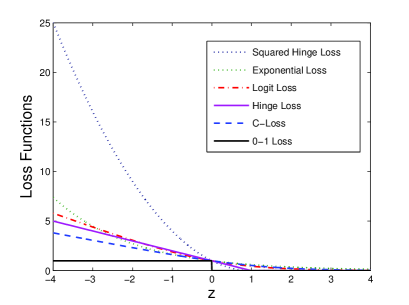
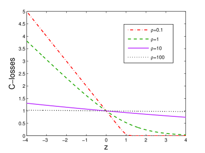
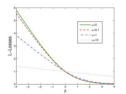
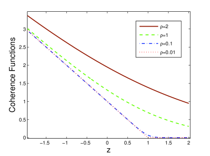
This proposition is depicted in Figure 1. Owing to the relationships of the $C$-loss $C_{{\rho},1}(yf(x))$ with the hinge and logit losses, it is potentially useful in devising new large-margin classifiers.

(a)	(b)
(c)	(d)

Figure 1: These functions are regarded as a function of $z=yf({\bf x})$. (a) Coherence functions $V_{{\rho},1}(z)$ with ${\rho}=0.01$, ${\rho}=0.1$, ${\rho}=1$ and ${\rho}=2$. (b)   A variety of majorization loss functions, $C$-loss: $C_{1,1}(z)$; Logit loss: $L_{1,0}(z)$; Exponential loss: $\exp({-}z/2)$; Hinge loss: $[1{-}z]_{+}$; Squared Hinge Loss: $([1{-}z]_{+})^{2}$. (c)   $C_{{\rho},1}(z)$ (or $L_{{\rho},1}(z)$) with ${\rho}=0.1$, ${\rho}=1$, ${\rho}=10$ and ${\rho}=100$ (see Proposition 3-(i)). (d)   $L_{1,u}(z)$ with $u=0$, $u=0.1$, $u=1$ and $u=10$ (see Proposition 3-(ii)).

We now turn to the derivatives of $C_{{\rho},u}(z)$ and $(u{-}z)_{+}$. It is immediately verified that $-1\leq C^{\prime}_{{\rho},u}(z)\leq 0$. Moreover, we have

$$\lim_{{\rho}\rightarrow 0}C^{\prime}_{{\rho},u}(z)=\lim_{{\rho}\rightarrow 0}V^{\prime}_{{\rho},u}(z)=\left\{\begin{array}[]{ll}0&z>u,\\ -\frac{1}{2}&z=u,\\ -1&z<u.\end{array}\right.$$

Note that $(u{-}z)_{+}^{\prime}=-1$ if $z<u$ and $(u{-}z)_{+}^{\prime}=0$ if $z>u$. Furthermore, $\partial(u{-}z)_{+}|_{z=u}=[-1,0]$ where $\partial(u{-}z)_{+}|_{z=u}$ denotes the subdifferential of $(u{-}z)_{+}$ at $z=u$. Hence,

Proposition 5

For a fixed $u>0$, we have that $\lim_{{\rho}\rightarrow 0}C^{\prime}_{{\rho},u}(z)\in\;\partial(u{-}z)_{+}$.

This proposition again establishes a connection of the hinge loss with the limit of $C_{{\rho},u}(z)$ at ${\rho}=0$. Furthermore, we obtain from Propositions 2 and 5 that $\partial(u{-}z)_{+}=\partial\lim_{{\rho}\rightarrow 0}C_{{\rho},u}(z)\ni\lim_{{\rho}\rightarrow 0}\partial C_{{\rho},u}(z)$.

3.3 Consistency in Classification Methods

We now apply the coherence function to the development of classification methods. Recall that $C_{{\rho},u}^{\prime}(0)$ exists and is negative. Thus, the $C$-loss $C_{{\rho},u}(yf(x))$ is Fisher-consistent (or classification calibrated) (Bartlett et al., 2006). In particular, we have the following theorem.

Theorem 6

Assume $0<\eta<1$ and $\eta\neq\frac{1}{2}$. Consider the optimization problem

$$\min_{f\in{\mathbb{R}}}\;R(f,\eta):=V_{{\rho},u}(f)\eta+V_{{\rho},u}(-f)(1-\eta)$$

for fixed ${\rho}>0$ and $u\geq 0$. Then, the minimizer is unique and is given by

$$f_{*}(\eta)={\rho}\log\frac{(2\eta{-}1)\exp(\frac{u}{{\rho}})+\sqrt{(1{-}2\eta)^{2}\exp(\frac{2u}{{\rho}})+4\eta(1{-}\eta)}}{2(1-\eta)}.$$ (9)

Moreover, we have $f_{*}>0$ if and only if $\eta>1/2$. Additionally, the inverse function $f_{*}^{-1}(f)$ exists and it is given by

$$\tilde{\eta}(f):=f_{*}^{-1}(f)=\frac{1+\exp(\frac{f-u}{{\rho}})}{1+\exp(-\frac{u+f}{{\rho}})+1+\exp(\frac{f-u}{{\rho}})},\;\;\mbox{for }\;f\in{\mathbb{R}}.$$ (10)

The minimizer $f_{*}({\bf x})$ of $R(f({\bf x})):={\mathbb{E}}(V_{{\rho},u}(Yf(X))|X={\bf x})$ and its inverse $\tilde{\eta}({\bf x})$ are immediately obtained by replacing $f$ with $f({\bf x})$ in (9) and (10). Since for $u>0$ the minimizers of ${\mathbb{E}}(C_{{\rho},u}(Yf(X))|X={\bf x})$ and ${\mathbb{E}}({V}_{{\rho},u}(Yf(X))|X={\bf x})$ are the same, this theorem shows that ${C}_{{\rho}}(yf({\bf x}),u)$ is also Fisher-consistent. We see from Theorem 6 that the explicit expressions of $f_{*}({\bf x})$ and its inverse $\tilde{\eta}({\bf x})$ exist. In the special case that $u=0$, we have $f_{*}({\bf x})={\rho}\log\frac{\eta({\bf x})}{1-\eta({\bf x})}$ and $\tilde{\eta}({\bf x})=\frac{1}{1+\exp(-{f}({\bf x})/{\rho})}$. Furthermore, when ${\rho}=1$, as expected, we recover logistic regression. In other words, the result is identical with that in Proposition 1 for logistic regression.

We further consider properties of $f_{*}(\eta)$. In particular, we have the following proposition.

Proposition 7

Let $f_{*}(\eta)$ be defined by (9). Then,

1. $\mathrm{sign}(f_{*}(\eta))=\mathrm{sign}({\eta}{-}1/2)$.

2. $\lim_{{\rho}\rightarrow 0}f_{*}(\eta)=u{\times}{\mathrm{sign}}(\eta-1/2)$.

3. $f_{*}^{\prime}(\eta)=\frac{df_{*}(\eta)}{d\eta}\geq\frac{{\rho}}{\eta(1-\eta)}$ with equality if and only if $u=0$.

Proposition 7-(i) shows that the classification rule with $f_{*}({\bf x})$ is equivalent to the Bayes rule. In the special case that $u=1$, we have from Proposition 7-(ii) that $\lim_{{\rho}\rightarrow 0}f_{*}({\bf x})={\mathrm{sign}}(\eta({\bf x})-1/2)$. This implies that the current $f_{*}({\bf x})$ approaches the solution of ${\mathbb{E}}((1-Yf(X))_{+}|X={\bf x})$, which corresponds to the conventional SVM method (see Proposition 1).

We now treat $\tilde{\eta}(f)$ as a function of ${\rho}$. The following proposition is easily proven.

Proposition 8

Let $\tilde{\eta}(f)$ be defined by (10). Then, for fixed $f\in{\mathbb{R}}$ and $u>0$, $\lim_{{\rho}\rightarrow\infty}\tilde{\eta}(f)=\frac{1}{2}$ and

$$\lim_{{\rho}\rightarrow 0}\tilde{\eta}(f)=\left\{\begin{array}[]{l@{\quad}l}1&\mbox{if }f>u,\\ \frac{2}{3}&\mbox{if }f=u,\\ \frac{1}{2}&\mbox{if }-u<f<u,\\ \frac{1}{3}&\mbox{if }f=-u,\\ 0&\mbox{if }f<-u.\end{array}\right.$$

As we discuss in the previous subsection, $V_{{\rho},u}(z)$ is obtained when setting $w=\exp((u{-}z)/{\rho})/(1+\exp((u{-}z)/{\rho}))$ by using the maximum entropy principle. Let $z=yf({\bf x})$. We further write $w$ as $w_{1}(f)=1/[1+\exp((f{-}u)/{\rho})]$ when $y=1$ and as $w_{2}(f)=1/[1+\exp(-(f{+}u)/{\rho})]$ when $y=-1$.

We now explore the relationship of $\tilde{\eta}(f)$ with $w_{1}(f)$ and $w_{2}(f)$. Interestingly, we first find that

$$\tilde{\eta}(f)=\frac{w_{2}(f)}{w_{1}(f)+w_{2}(f)}.$$

It is easily proven that $w_{1}(f)+w_{2}(f)\geq 1$ with equality if and only if $u=0$. We thus have that $\tilde{\eta}(f)\leq w_{2}(f)$, with equality if and only if $u=0$; that is, the loss becomes logit function $V_{{\rho},0}(z)$. Note that $w_{2}(f)$ represents the probability of the event $\{u+f>0\}$ and $\tilde{\eta}(f)$ represents the probability of the event $\{f>0\}$. Since the event $\{f>0\}$ is a subset of the event $\{u+f>0\}$, we have $\tilde{\eta}(f)\leq w_{2}(f)$. Furthermore, the statement that $\tilde{\eta}(f)=w_{2}(f)$ if and only if $u=0$ is equivalent to $\{u+f>0\}=\{f>0\}$ if and only if $u=0$. This implies that only the logit loss induces $\tilde{\eta}(f)=w_{2}(f)$.

As discussed in Section 2.1, $\tilde{\eta}({\bf x})$ can be regarded as a reasonable estimate of the true class probability $\eta({\bf x})$. Recall that $\triangle R(\eta,f)=R(\eta,f)-R(\eta,f_{*}(\eta))$ and $\triangle R_{f}={\mathbb{E}}_{X}[\triangle R(\eta(X),f(X))]$ such that $\triangle R_{f}$ can be viewed as the expected distance between $\tilde{\eta}({\bf x})$ and $\eta({\bf x})$.

For an arbitrary fixed $f\in{\mathbb{R}}$, we have

$$\triangle R(\eta,f)=R(\eta,f)-R(\eta,f_{*}(\eta))=\eta{\rho}\log\frac{1+\exp\frac{u{-}f}{{\rho}}}{1+\exp\frac{u{-}f_{*}(\eta)}{{\rho}}}+(1-\eta){\rho}\log\frac{1+\exp\frac{u{+}f}{{\rho}}}{1+\exp\frac{u{+}f_{*}(\eta)}{{\rho}}}.$$

The first-order derivative of $\triangle R(\eta,f)$ with respect to $\eta$ is

$$\frac{d\triangle R(\eta,f)}{d\eta}={\rho}\log\frac{1+\exp\frac{u{-}f}{{\rho}}}{1+\exp\frac{u{-}f_{*}(\eta)}{{\rho}}}-{\rho}\log\frac{1+\exp\frac{u{+}f}{{\rho}}}{1+\exp\frac{u{+}f_{*}(\eta)}{{\rho}}}.$$

The Karush-Kuhn-Tucker (KKT) condition for the minimization problem is as follows:

$$\eta\frac{\exp\frac{u{-}f_{*}(\eta)}{{\rho}}}{1{+}\exp\frac{u{-}f_{*}(\eta)}{{\rho}}}+(1-\eta)\frac{\exp\frac{u{+}f_{*}(\eta)}{{\rho}}}{1{+}\exp\frac{u{+}f_{*}(\eta)}{{\rho}}}=0,$$

and the second-order derivative of $\triangle R(\eta,f)$ with respect to $\eta$ is given by

$$\frac{d^{2}\triangle R(\eta,f)}{d\eta^{2}}=\Big{(}\frac{1}{1+\exp({-}\frac{u{-}f_{*}(\eta)}{{\rho}})}+\frac{1}{1+\exp({-}\frac{u{+}f_{*}(\eta)}{{\rho}})}\Big{)}f_{*}^{\prime}(\eta)=\big{[}w_{1}(f_{*}(\eta))+w_{2}(f_{*}(\eta))\big{]}f_{*}^{\prime}(\eta).$$

According to Proposition 7-(iii) and using $w_{1}(f_{*}(\eta))+w_{2}(f_{*}(\eta))\geq 1$, we have

$$\frac{d^{2}\triangle R(\eta,f)}{d\eta^{2}}\geq\frac{{\rho}}{\eta(1-\eta)},$$

with equality if and only if $u=0$. This implies $\frac{d^{2}\triangle R(\eta,f)}{d\eta^{2}}>0$. Thus, for a fixed $f$, $\triangle R(\eta,f)$ is strictly convex in $\eta$. Subsequently, we have that $\triangle R(\eta,f)\geq 0$ with equality $\eta=\tilde{\eta}$, or equivalently, $f=f_{*}$.

Using the Taylor expansion of $\triangle R(\eta,f)$ at $\tilde{\eta}:=\tilde{\eta}(f)=f_{*}^{-1}(f)$, we thus obtain a lower bound for $\triangle R(\eta,f)$; namely,

$$\triangle R(\eta,f) =\triangle R(\tilde{\eta},f)-\frac{d\triangle R(\tilde{\eta},f)}{d\eta}(\eta-\tilde{\eta})+\frac{1}{2}\frac{d^{2}\triangle R(\bar{\eta},f)}{d\eta^{2}}(\eta-\tilde{\eta})^{2}$$

$$=\frac{1}{2}\frac{d^{2}\triangle R(\bar{\eta},f)}{d\eta^{2}}(\eta-\tilde{\eta})^{2}\geq\frac{{\rho}}{2\bar{\eta}(1-\bar{\eta})}(\eta-\tilde{\eta})^{2}\geq 2{\rho}(\eta-\tilde{\eta})^{2},$$

where $\bar{\eta}\in(\tilde{\eta},\eta)\subset[0,1]$. In particular, we have that $\triangle R(\eta,0)\geq 2{\rho}(\eta-0.5)^{2}$. According to Theorem 2.1 and Corollary 3.1 in Zhang (2004), the following theorem is immediately established.

Theorem 9

Let $\epsilon_{1}=\inf_{f(\cdot)\in{\mathcal{F}}}{\mathbb{E}}_{X}[\triangle R(\eta(X),f(X))]$, and let $f_{*}({\bf x})\in{\mathcal{F}}$ such that

$${\mathbb{E}}_{X}[R(\eta(X),f_{*}(X))]\leq\inf_{f(\cdot)\in{\mathcal{F}}}{\mathbb{E}}_{X}[R(\eta(X),{f}(X))]+\epsilon_{2}$$

for $\epsilon_{2}\geq 0$. Then for $\epsilon=\epsilon_{1}+\epsilon_{2}$,

$$\triangle R_{f_{*}}={\mathbb{E}}_{X}[\triangle R(\eta(X),f_{*}(X))]\leq\epsilon$$

and

$$\Psi_{f_{*}}\leq\hat{\Psi}+\big{(}2\epsilon/{\rho}\big{)}^{1/2},$$

where $\Psi_{f_{*}}={\mathbb{E}}_{P}I_{[Yf_{*}(X)\leq 0]}$, and $\hat{\Psi}={\mathbb{E}}_{P}I_{[Y(2\eta(X){-}1)\leq 0]}$ is the optimal Bayes error.

3.4 Analysis

For notational simplicity, we will use $C_{{\rho}}(z)$ for $C_{{\rho},1}(z)$. Considering $f({\bf x})=\alpha+\mbox{\boldmath$\beta$\unboldmath}^{\prime}{\bf k}$, we define an regularized optimization problem of the form

$$\min_{\alpha,\;\mbox{\boldmath$\beta$\unboldmath}}\Big{\{}\frac{1}{n}\sum_{i=1}^{n}C_{{\rho}}(y_{i}f({\bf x}_{i}))+\frac{\gamma_{n}}{2}\mbox{\boldmath$\beta$\unboldmath}^{\prime}{\bf K}\mbox{\boldmath$\beta$\unboldmath}\Big{\}}.$$ (11)

Here we assume that the regularization parameter $\gamma$ relies on the number $n$ of training data points, thus we denote it by $\gamma_{n}$.

Since the optimization problem (11) is convex with respect to $\alpha$ and $\beta$, the solution exists and is unique. Moreover, since $C_{\rho}$ is infinitely smooth, we can resort to the Newton-Raphson method to solve (11).

Proposition 10

Assume that $\gamma_{n}$ in (11) and $\gamma$ in (4) are same. Then the minimizer of (11) approaches the minimizer of (4) as ${\rho}\rightarrow 0$.

This proposition is obtained directly from Proposition 5. For a fixed ${\rho}$, we are also concerned with the universal consistency of the classifier based on (11) with and without the offset term $\alpha$.

Theorem 11

Let $K(\cdot,\cdot)$ be a universal kernel on ${\mathcal{X}}{\times}{\mathcal{X}}$. Suppose we are given such a positive sequence $\{\gamma_{n}\}$ that $\gamma_{n}\rightarrow 0$. If

$$n\gamma^{2}_{n}/\log n\rightarrow\infty,$$

then the classifier based on (11) is strongly universally consistent. If

$$n\gamma^{2}_{n}\rightarrow\infty,$$

then the classifier based on (11) with $\alpha=0$ is universally consistent.

3.5 Class Probability Estimation of SVM Outputs

As discussed earlier, the limit of the coherence function, $V_{{\rho},1}(yf({\bf x}))$, at ${\rho}=0$ is just the hinge loss. Moreover, Proposition 7 shows that the minimizer of $V_{{\rho},1}(f)\eta+V_{{\rho},1}(-f)(1{-}\eta)$ approaches that of $H(f)\eta+H(-f)(1{-}\eta)$ as ${\rho}\rightarrow 0$. Thus, Theorem 6 provides us with an approach to the estimation of the class probability for the conventional SVM.

In particular, let $\hat{f}({\bf x})$ be the solution of the optimization problem (4) for the conventional SVM. In terms of Theorem 6, we suggest that the estimated class probability $\hat{\eta}({\bf x})$ is defined as

$$\hat{\eta}({\bf x})=\frac{1+\exp(\frac{\hat{f}({\bf x})-1}{{\rho}})}{1+\exp(-\frac{1+\hat{f}({\bf x})}{{\rho}})+1+\exp(\frac{\hat{f}({\bf x})-1}{{\rho}})}.$$ (12)

Proposition 7 would seem to motivate setting $\rho$ to a very small value in (12). However, as shown in Proposition 8, the probabilistic outputs degenerate to $0$, $1/3$, $1/2$, $2/3$ and $1$ in this case. Additionally, the classification function $\hat{f}({\bf x})=\hat{\alpha}+\sum_{i=1}^{n}\hat{\beta}_{i}K({\bf x},{\bf x}_{i})$ is obtained via fitting a conventional SVM model on the training data. Thus, rather than attempting to specify a fixed value of $\rho$ via a theoretical argument, we instead view it as a hyperparameter to be fit empirically.

In particular, we fit ${\rho}$ by minimizing the generalized Kullback-Leibler divergence (or cross-entropy error) between $\hat{\eta}(X)$ and $\eta(X)$, which is given by

$$\mbox{GKL}(\eta,\hat{\eta})={\mathbb{E}}_{X}\Big{[}\eta(X)\log\frac{\eta(X)}{\hat{\eta}(X)}+(1{-}\eta(X))\log\frac{1{-}\eta(X)}{1{-}\hat{\eta}(X)}\Big{]}.$$

Alternatively, we formulate the optimization problem for obtaining ${\rho}$ as

$$\min_{{\rho}>0}\;\mbox{EKL}(\hat{\eta}):=-\frac{1}{n}\sum_{i=1}^{n}\Big{\{}\frac{1}{2}(y_{i}+1)\log\hat{\eta}({\bf x}_{i})+\frac{1}{2}(1-y_{i})\log(1-\hat{\eta}({\bf x}_{i}))\Big{\}}.$$ (13)

The problem can be solved by the Newton method. In summary, one first obtains $\hat{f}({\bf x})=\hat{\alpha}+\sum_{i=1}^{n}\hat{\beta}_{i}K({\bf x},{\bf x}_{i})$ via the conventional SVM model, and estiamtes $\rho$ via the optimization problem in (13) based on the training data; one then uses the formula in (12) to estimate the class probabilities for the training samples as well as the test samples.

4 ${\cal C}$-Learning

Focusing on the relationships of the $C$-loss $C_{{\rho}}(yf(x))$ (i.e., $C_{{\rho},1}(yf(x))$) with the hinge and logit losses, we illustrate its application in the construction of large-margin classifiers. Since $C_{\rho}(yf({\bf x}))$ is smooth, it does not tend to yield a sparse classifier. However, we can employ a sparsification penalty $J(h)$ to arrive at sparseness. We use the elastic-net penalty of Zou and Hastie (2005) for the experiments in this section. Additionally, we study two forms of $f({\bf x})$: kernel expansion and feature expansion. Built on these two expansions, sparseness can subserve the selection of support vectors and the selection of features, respectively. The resulting classifiers are called ${\cal C}$-learning.

4.1 The Kernel Expansion

In the kernel expansion approach, given a reproducing kernel $K(\cdot,\cdot):$ ${\mathcal{X}}\times{\mathcal{X}}\rightarrow{\mathbb{R}}$, we define the kernel expansion as $f({\bf x})=\alpha+\sum_{i=1}^{n}\beta_{i}K({\bf x}_{i},{\bf x})$ and solve the following optimization problem:

$$\min_{\alpha,\mbox{\boldmath$\beta$\unboldmath}}\frac{1}{n}\sum_{i=1}^{n}C_{{\rho}}(y_{i}f({\bf x}_{i}))+\gamma\Big{(}(1{-}\omega)\frac{1}{2}\mbox{\boldmath$\beta$\unboldmath}^{\prime}{\bf K}\mbox{\boldmath$\beta$\unboldmath}+\omega\|\mbox{\boldmath$\beta$\unboldmath}\|_{1}\Big{)},$$ (14)

where ${\bf K}=[K({\bf x}_{i},{\bf x}_{j})]$ is the $n{\times}n$ kernel matrix.

It is worth pointing out that the current penalty is slightly different from the conventional elastic-net penalty, which is $(1{-}\omega)\frac{1}{2}\mbox{\boldmath$\beta$\unboldmath}^{\prime}\mbox{\boldmath$\beta$\unboldmath}+\omega\|\mbox{\boldmath$\beta$\unboldmath}\|_{1}$. In fact, the optimization problem (14) can be viewed equivalently as the optimization problem

$$\min_{\alpha,\mbox{\boldmath$\beta$\unboldmath}}\frac{1}{n}\sum_{i=1}^{n}C_{{\rho}}(y_{i}f({\bf x}_{i}))+\frac{\gamma}{2}\mbox{\boldmath$\beta$\unboldmath}^{\prime}{\bf K}\mbox{\boldmath$\beta$\unboldmath}$$ (15)

under the $\ell_{1}$ penalty $\|\mbox{\boldmath$\beta$\unboldmath}\|_{1}$. Thus, the method derived from (14) enjoys the generalization ability of the conventional kernel supervised learning method derived from (15) but also the sparsity of the $\ell_{1}$ penalty.

Recently, Friedman et al. (2010) devised a pathwise coordinate descent algorithm for regularized logistic regression problems in which the elastic-net penalty is used. In order to solve the optimization problem in (14), we employ this pathwise coordinate descent algorithm.

Let the current estimates of $\alpha$ and $\beta$ be $\hat{\alpha}$ and $\hat{\beta}$. We first form a quadratic approximation to $\frac{1}{n}\sum_{i=1}^{n}C_{{\rho}}(y_{i}f({\bf x}_{i}))$, which is

$${Q}(\alpha,\mbox{\boldmath$\beta$\unboldmath})=\frac{1}{2n\rho}\sum_{i=1}^{n}q({\bf x}_{i})(1-q({\bf x}_{i}))\big{(}\alpha+{\bf k}_{i}^{\prime}\mbox{\boldmath$\beta$\unboldmath}-z_{i}\big{)}^{2}+\mbox{Const},$$ (16)

where

$$z_{i} = \hat{\alpha}+{\bf k}_{i}^{\prime}\hat{\mbox{\boldmath$\beta$\unboldmath}}+\frac{{\rho}}{y_{i}(1-q({\bf x}_{i}))},$$

$$q({\bf x}_{i}) = \frac{\exp[(1-y_{i}(\hat{\alpha}+{\bf k}_{i}^{\prime}\hat{\mbox{\boldmath$\beta$\unboldmath}})/{\rho}]}{1+\exp[(1-y_{i}(\hat{\alpha}+{\bf k}_{i}^{\prime}\hat{\mbox{\boldmath$\beta$\unboldmath}}))/{\rho}]},$$

$${\bf k}_{i} = (K({\bf x}_{1},{\bf x}_{i}),\ldots,K({\bf x}_{n},{\bf x}_{i}))^{\prime}.$$

We then employ coordinate descent to solve the weighted least-squares problem as follows:

$$\min_{\alpha,\mbox{\boldmath$\beta$\unboldmath}}\;G(\alpha,\mbox{\boldmath$\beta$\unboldmath}):={Q}(\alpha,\mbox{\boldmath$\beta$\unboldmath})+\gamma\Big{(}(1{-}\omega)\frac{1}{2}\mbox{\boldmath$\beta$\unboldmath}^{\prime}{\bf K}\mbox{\boldmath$\beta$\unboldmath}+\omega\|\mbox{\boldmath$\beta$\unboldmath}\|_{1}\Big{)}.$$ (17)

Assume that we have estimated $\tilde{\mbox{\boldmath$\beta$\unboldmath}}$ for $\beta$ using $G(\alpha,\mbox{\boldmath$\beta$\unboldmath})$. We now set $\frac{\partial G(\alpha,\tilde{\mbox{\boldmath$\beta$\unboldmath}})}{\partial\alpha}=0$ to find the new estimate of $\alpha$:

$$\tilde{\alpha}=\frac{\sum_{i=1}^{n}q({\bf x}_{i})(1-q({\bf x}_{i}))\big{(}z_{i}-{\bf k}_{i}^{\prime}\tilde{\mbox{\boldmath$\beta$\unboldmath}}\big{)}}{\sum_{i=1}^{n}q({\bf x}_{i})(1-q({\bf x}_{i}))}.$$ (18)

On the other hand, assume that we have estimated $\tilde{\alpha}$ for $\alpha$ and $\tilde{\beta}_{l}$ for $\beta_{l}$ $(l=1,\ldots,n,l\neq j)$. We now optimize ${\beta}_{j}$. In particular, we only consider the gradient at $\beta_{j}\neq 0$. If $\beta_{j}>0$, we have

$$\frac{\partial G(\tilde{\alpha},\tilde{\mbox{\boldmath$\beta$\unboldmath}})}{\partial\beta_{j}}=\frac{1}{n{\rho}}\sum_{i=1}^{n}K_{ij}q({\bf x}_{i})(1-q({\bf x}_{i}))\big{(}\alpha{+}{\bf k}_{i}^{\prime}\tilde{\mbox{\boldmath$\beta$\unboldmath}}{-}z_{i}\big{)}+\gamma(1{-}\omega)(K_{jj}\beta_{j}{+}{\bf k}_{j}\check{\mbox{\boldmath$\beta$\unboldmath}})+\gamma\omega$$

and, hence,

$$\tilde{\beta_{j}}=\frac{S(t-\gamma(1-\omega){\bf k}_{j}^{\prime}\check{\mbox{\boldmath$\beta$\unboldmath}},\gamma\omega)}{\frac{1}{n{\rho}}\sum_{i=1}^{n}K_{ij}^{2}q({\bf x}_{i})(1-q({\bf x}_{i}))+\gamma(1-\omega)K_{jj}},$$ (19)

where $t=\frac{1}{n\rho}\sum_{i=1}^{n}K_{ij}q({\bf x}_{i})(1-q({\bf x}_{i}))\big{(}z_{i}-\tilde{\alpha}-{\bf k}_{i}^{\prime}\check{\mbox{\boldmath$\beta$\unboldmath}}\big{)}$, $\check{\mbox{\boldmath$\beta$\unboldmath}}=(\tilde{\beta}_{1},\ldots,\tilde{\beta}_{j-1},0,\tilde{\beta}_{j+1},\ldots,\tilde{\beta}_{n})^{\prime}$, $K_{ij}=K({\bf x}_{i},{\bf x}_{j})$, and $S(\mu,\nu)$ is the soft-thresholding operator:

$$S(\mu,\nu) =\mathrm{sign}(\mu)(|\mu|-\nu)_{+}$$

$$=\left\{\begin{array}[]{ll}\mu-\nu&\mbox{if }\mu>0\mbox{ and }\mu<|\nu|\\ \mu+\nu&\mbox{if }\mu<0\mbox{ and }\mu<|\nu|\\ 0&\mbox{if }\mu>|\nu|.\end{array}\right.$$

Algorithm 1 summarizes the coordinate descent algorithm for binary $C$-learning.

Algorithm 1 The coordinate descent algorithm for binary ${\cal C}$-learning

  Input: ${\mathcal{T}}=\{{\bf x}_{i},y_{i}\}_{i=1}^{n}$, $\gamma$, $\omega$, $\epsilon_{m}$, $\epsilon_{i}$, ${\rho}$;

  Initialize: $\tilde{\alpha}=\alpha_{0}$, $\tilde{\mbox{\boldmath$\beta$\unboldmath}}=\mbox{\boldmath$\beta$\unboldmath}_{0}$

  repeat

     Calculate $G(\tilde{\alpha},\tilde{\mbox{\boldmath$\beta$\unboldmath}})$ using (17);

     $\alpha^{\star}\leftarrow\tilde{\alpha}$;

     $\mbox{\boldmath$\beta$\unboldmath}^{\star}\leftarrow\tilde{\mbox{\boldmath$\beta$\unboldmath}}$;

     repeat

        $\bar{\alpha}\leftarrow\tilde{\alpha}$;

        $\bar{\mbox{\boldmath$\beta$\unboldmath}}\leftarrow\tilde{\mbox{\boldmath$\beta$\unboldmath}}$;

        Calculate $\tilde{\alpha}$ using (18);

        for $j=1$ to $n$ do

           Calculate $\tilde{\beta}_{j}$ using (19);

        end for

     until $\|\tilde{\alpha}-\bar{\alpha}\|+\|\tilde{\mbox{\boldmath$\beta$\unboldmath}}-\bar{\mbox{\boldmath$\beta$\unboldmath}}\|<\epsilon_{i}$

  until $\|\tilde{\alpha}-\alpha^{\star}\|+\|\tilde{\mbox{\boldmath$\beta$\unboldmath}}-\mbox{\boldmath$\beta$\unboldmath}^{\star}\|<\epsilon_{m}$

  Output: $\tilde{\alpha}$, $\tilde{\mbox{\boldmath$\beta$\unboldmath}}$, and $f({\bf x})=\tilde{\alpha}+\sum_{i=1}^{n}K({\bf x}_{i},{\bf x})\tilde{\beta_{i}}$.

4.2 The Linear Feature Expansion

In the linear feature expansion approach, we let $f({\bf x})=a+{\bf x}^{\prime}{\bf b}$, and pose the following optimization problem:

$$\min_{a,{\bf b}}\frac{1}{n}\sum_{i=1}^{n}C_{{\rho}}(y_{i}f({\bf x}_{i}))+\gamma J_{\omega}({\bf b}),$$ (20)

where for $\omega\in[0,1]$

$$J_{\omega}({\bf b}) =(1-\omega)\frac{1}{2}\|{\bf b}\|^{2}_{2}+\omega\|{\bf b}\|_{1}=\sum_{j=1}^{d}\Big{[}\frac{1}{2}(1-\omega)b_{j}^{2}+\omega|b_{j}|\Big{]}.$$

The elastic-net penalty maintains the sparsity of the $\ell_{1}$ penalty, but the number of variables to be selected is no longer bounded by $n$. Moreover, this penalty tends to generate similar coefficients for highly-correlated variables. We also use a coordinate descent algorithm to solve the optimization problem (20). The algorithm is similar to that for the kernel expansion and the details are omitted here.

5 Experimental Results

In Section 5.1 we report the results of experimental evaluations of our method for class probability estimation of the conventional SVM given in Section 3.5. In Section 5.2 we present results for the ${\mathcal{C}}$-learning method given in Section 4.

5.1 Simulation for Class Probability Estimation of SVM Outputs

We validate our estimation method for the class probability of SVM outputs (“Ours for SVM”), comparing it with several alternatives: Platt’s method (Platt, 1999), Sollich’s method (Sollich, 2002), and the method of Wang et al. (2008) (WSL’s). Since penalized (or regularized) logistic regression (PLR) and ${\mathcal{C}}$-learning can directly calculate class probability, we also implement them. Especially, the class probability of ${\mathcal{C}}$-learning outputs is based on (10) where we set $\rho=1$ and $u=1$ since ${\mathcal{C}}$-learning itself employs the same setting.

We conducted our analysis over two simulation datasets which were used by Wang et al. (2008). The first simulation dataset, $\{(x_{i1},x_{i2};y_{i})\}_{i=1}^{1000}$, was generated as follows. The $\{(x_{i1},x_{i2})\}_{i=1}^{1000}$ were uniformly sampled from a unit disk $\{(x_{1},x_{2}):x^{2}_{1}+x^{2}_{2}\leq 1\}$. Next, we set $y_{i}=1$ if $x_{i1}\geq 0$ and $y_{i}=-1$ otherwise, $i=1,\ldots,1000$. Finally, we randomly chose $20\%$ of the samples and flipped their labels. Thus, the true class probability $\eta(Y_{i}=1|x_{i1},x_{i2})$ was either 0.8 or 0.2.

The second dataset, $\{(x_{i1},x_{i2};y_{i})\}_{i=1}^{1000}$, was generated as follows. First, we randomly assigned $1$ or $-1$ to $y_{i}$ for $i=1,\ldots,1000$ with equal probability. Next, we generated $x_{i1}$ from the uniform distribution over $[0,2\pi]$, and set $x_{i2}=y_{i}(\sin(x_{i1})+\epsilon_{i})$ where $\epsilon_{i}\sim N(\epsilon_{i}|1,0.01)$. For the data, the true class probability of $Y=1$ was given by

$$\eta(Y=1|x_{1},x_{2})=\frac{N(x_{2}|\sin(x_{1}){+}1,0.01)}{N(x_{2}|\sin(x_{1}){+}1,0.01)+N(x_{2}|-\sin(x_{1}){-}1,0.01)}.$$

The simulation followed the same setting as that in Wang et al. (2008). That is, we randomly selected 100 samples for training and the remaining 900 samples for test. We did 100 replications for each dataset. The values of generalized Kullback-Leibler loss (GKL) and classification error rate (CER) on the test sets were averaged over these 100 simulation replications. Additionally, we employed a Gaussian RBF kernel $K({\bf x}_{i},{\bf x}_{j})=\exp(-\|{\bf x}_{i}-{\bf x}_{j}\|^{2}/\sigma^{2})$ where the parameter $\sigma$ was set as the median distance between the positive and negative classes. We reported GKL and CER as well as the corresponding standard deviations in Tables 2 and 3 in which the results with the PLR method, the tuned Platt method and the WSL method are directly cited from Wang et al. (2008).

Note that the results with PLR were averaged only over 66 nondegenerate replications (Wang et al., 2008). Based on GKL and CER, the performance of ${\mathcal{C}}$-learning is the best in these two simulations. With regard to GKL, our method for SVM outperforms the original and tuned versions of Platt’s method as well as the method of Wang et al. (2008). Since our estimation method is based on the $\hat{\eta}({\bf x})$ in (12), the CER with this class probability $\hat{\eta}({\bf x})$ is identical to that with the conventional SVM. This also applies to Sollich’s method, thus we did not include the CER with this method. However, Table 3 shows that this does not necessarily hold for Platt’s method for SVM probability outputs. In other words, $\hat{\eta}({\bf x})>1/2$ is not equivalent to $\hat{f}({\bf x})>0$ for Platt’s method. In fact, Platt (1999) used this sigmoid-like function to improve the classification accuracy of the conventional SVM. As for the method of Wang et al. (2008) which is built on a sequence of weighted classifiers, the CERs of the method should be different from those of the original SVM. With regard to CER, the performance of PLR is the worst in most cases.

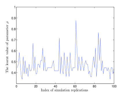
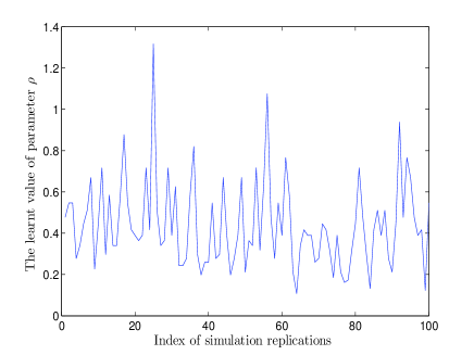
In addition, Figure 2 plots the estimated values of parameter $\rho$ with respect to the 100 simulation replications in our method for class probability estimation of the original SVM. For simulation 1, the estimated values of $\rho$ range from 0.3402 to 0.8773, while they range from 0.1077 to 1.3166 for simulation 2.

Table 2: Values of GKL over the two simulation test sets (standard deviations are shown in parentheses).

	PLR	Platt’s	Tuned Platt	WSL’s	Sollich’s	Ours for SVM	${\mathcal{C}}$-learning
Data 1	0.579	0.582	0.569	0.566	0.566	0.558	0.549
	($\pm 0.0021$)	($\pm 0.0035$)	($\pm 0.0015$)	($\pm 0.0014$)	($\pm 0.0021$)	($\pm 0.0015$)	($\pm 0.0016$)
Data 2	0.138	0.163	0.153	0.153	0.155	0.142	0.134
	($\pm 0.0024$)	($\pm 0.0018$)	($\pm 0.0013$)	($\pm 0.0010$)	($\pm 0.0017$)	($\pm 0.0016$)	($\pm 0.0014$)

Table 3: Values of CER over the two simulation test sets (standard deviations are shown in parentheses).

	PLR	Platt’s	WSL’s	Ours for SVM	${\mathcal{C}}$-learning
Data 1	0.258	0.234	0.217	0.219	0.214
	($\pm 0.0053$)	($\pm 0.0026$)	($\pm 0.0021$)	($\pm 0.0021$)	($\pm 0.0015$)
Data 2	0.075	0.077	0.069	0.065	0.061
	($\pm 0.0018$)	($\pm 0.0024$)	($\pm 0.0014$)	($\pm 0.0015$)	($\pm 0.0019$)

(a) Simulation 1	(b) Simulation 2

Figure 2: The learned values of parameter $\rho$ vs. simulation replications in our estimation method for the class probability of SVM outputs.

5.2 The Performance Analysis of ${\mathcal{C}}$-Learning

To evaluate the performance of our ${\mathcal{C}}$-learning method, we further conducted empirical studies on several benchmark datasets and compared ${\mathcal{C}}$-learning with two closely related classification methods: the hybrid huberized SVM (HHSVM) of Wang et al. (2007) and the regularized logistic regression model (RLRM) of Friedman et al. (2010), both with the elastic-net penalty. All the three classification methods were implemented in both the feature and kernel expansion settings.

In the experiments we used 11 binary classification datasets. Table 4 gives a summary of these benchmark datasets. The seven binary datasets of digits were obtained from the publicly available USPS dataset of handwritten digits as follows. The first six datasets were generated from the digit pairs {(1, 7), (2, 3), (2, 7), (3, 8), (4, 7), (6,9)}, and 200 digits were chosen within each class of each dataset is 200. The USPS (odd vs. even) dataset consisted of the first 80 images per digit in the USPS training set.

The two binary artificial datasets of “g241c” and “g241d” were generated via the setup presented by Chapelle et al. (2006). Each class of these two datasets consisted of 750 samples.

The two binary gene datasets of “colon” and “leukemia” were also used in our experiments. The “colon” dataset, consisting of 40 colon tumor samples and 22 normal colon tissue samples with 2,000 dimensions, was obtained by employing an Affymetrix oligonucleotide array to analyze more than 6,500 human genes expressed in sequence tags (Alon et al., 1999). The “leukemia” dataset is of the same type as the “colon” cancer dataset (Golub et al., 1999), and it was obtained with respect to two variants of leukemia, i.e., acute myeloid leukemia (AML) and acute lymphoblastic leukemia (ALL). It initially contained expression levels of 7129 genes taken over 72 samples (AML, 25 samples, or ALL, 47 samples), and then it was pre-feature selected, leading to a feature space with 3571 dimensions.

In our experiments, each dataset was randomly partitioned into two disjoint subsets as the training and test, with the percentage of the training data samples also given in Table 4. Twenty random partitions were chosen for each dataset, and the average and standard deviation of their classification error rates over the test data were reported.

Table 4: Summary of the benchmark datasets: $m$—the number of classes; $d$—the dimension of the input vector; $k$—the size of the dataset; $n$—the number of the training data.

Dataset	$m$	$d$	k	$n/k$
USPS (1 vs. 7)	2	256	400	3%
USPS (2 vs. 3)	2	256	400	3%
USPS (2 vs. 7)	2	256	400	3%
USPS (3 vs. 8)	2	256	400	3%
USPS (4 vs. 7)	2	256	400	3%
USPS (6 vs. 9)	2	256	400	3%
USPS (Odd vs. Even)	2	256	800	3%
g241c	2	241	1500	10%
g241d	2	241	1500	10%
colon	2	2000	62	25.8%
leukemia	2	3571	72	27.8%

Table 5: Classification error rates (%) and standard deviations on the 11 datasets for the feature expansion setting.

Dataset	HHSVM	RLRM	${\mathcal{C}}$-learning
(1 vs. 7)	2.29$\pm$1.17	2.06$\pm$1.21	1.60$\pm$0.93
(2 vs. 3)	8.13$\pm$2.02	8.29$\pm$2.76	8.32$\pm$2.73
(2 vs. 7)	5.82$\pm$2.59	6.04$\pm$2.60	5.64$\pm$2.44
(3 vs. 8)	12.46$\pm$2.90	10.77$\pm$2.72	11.74$\pm$2.83
(4 vs. 7)	7.35$\pm$2.89	6.91$\pm$2.72	6.68$\pm$3.53
(6 vs. 9)	2.32$\pm$1.65	2.15$\pm$1.43	2.09$\pm$1.41
(Odd vs. Even)	20.94$\pm$2.02	19.83$\pm$2.82	19.74$\pm$2.81
g241c	22.30$\pm$1.30	21.38$\pm$1.12	21.34$\pm$1.11
g241d	24.32$\pm$1.53	23.81$\pm$1.65	23.85$\pm$1.69
colon	14.57$\pm$1.86	14.47$\pm$2.02	12.34$\pm$1.48
leukemia	4.06$\pm$2.31	4.43$\pm$1.65	3.21$\pm$1.08

Table 6: Classification error rates (%) and standard deviations on the 11 datasets for the RBF kernel setting.

Dataset	HHSVM	RLRM	${\mathcal{C}}$-learning
(1 vs. 7)	1.73$\pm$1.64	1.39$\pm$0.64	1.37$\pm$0.65
(2 vs. 3)	8.55$\pm$3.36	8.45$\pm$3.38	8.00$\pm$3.32
(2 vs. 7)	5.09$\pm$2.10	4.02$\pm$1.81	3.90$\pm$1.79
(3 vs. 8)	12.09$\pm$3.78	10.58$\pm$3.50	10.36$\pm$3.52
(4 vs. 7)	6.74$\pm$3.39	6.92$\pm$3.37	6.55$\pm$3.28
(6 vs. 9)	2.12$\pm$0.91	1.74$\pm$1.04	1.65$\pm$0.99
(Odd vs. Even)	28.38$\pm$10.51	26.92$\pm$6.52	26.29$\pm$6.45
g241c	21.38$\pm$1.45	21.55$\pm$1.42	21.62$\pm$1.35
g241d	25.89$\pm$2.15	22.34$\pm$1.27	20.37$\pm$1.20
colon	14.26$\pm$2.66	14.79$\pm$2.80	13.94$\pm$2.44
leukemia	2.77$\pm$0.97	2.74$\pm$0.96	2.55$\pm$0.92

Although we can seek an optimum $\rho$ using computationally intensive methods such as cross-validation, the experiments showed that when $\rho$ takes a value in $[0.1,2]$, our method is always able to obtain promising performance. Here our reported results are based on the setting of $\rho=1$, due to the relationship of the ${\mathcal{C}}$-loss ${\mathcal{C}}(z)$ with the hinge loss $(1-z)_{+}$ and the logit loss $\log(1+\exp(-z))$ (see our analysis in Section 3 and Figure 1).

As for the parameters $\gamma$ and $\omega$, they were selected by cross-validation for all the classification methods. In the kernel expansion, the RBF kernel $K({\bf x}_{i},{\bf x}_{j})=\exp(-\|{\bf x}_{i}-{\bf x}_{j}\|^{2}/\sigma^{2})$ was employed, and $\sigma$ was set to the mean Euclidean distance among the input samples. For ${\mathcal{C}}$-learning, the other parameters were set as follows: $\epsilon_{m}=\epsilon_{i}=10^{-5}$.

Tables 5 and 6 show the test results corresponding to the linear feature expansion and RBF kernel expansion, respectively. From the tables, we can see that for the overall performance of ${\mathcal{C}}$-learning is slightly better than the two competing methods in the feature and kernel settings generally.

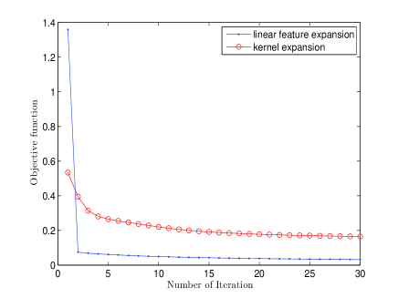
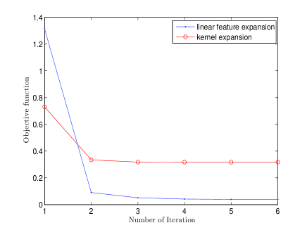
Figure 3 reveals that the values of the objective functions for the linear feature and RBF kernel versions in the outer and inner iterations tend to be significantly reduced as the number of iterations in the coordinate descent procedure increases. Although we report only the change of the values of the objective function for the dataset USPS (1 vs. 7) similar results were found on all other datasets. This shows that the coordinate descent algorithm is very efficient.

We also conducted a systematic study of sparseness from the elastic-net penalty. Indeed, the elastic-net penalty does give rise to sparse solutions for our ${\mathcal{C}}$-learning methods. Moreover, we found that similar to other methods the sparseness of the solution is dependent on the parameters $\gamma$ and $\omega$ that were set to different values for different datasets using cross validation.

(a)	(b)

Figure 3: Change of the value of the objective function for the ${\mathcal{C}}$-learning as the number of iterations in the coordinate descent procedure increases in the linear feature and RBF kernel cases on the dataset USPS (1 vs. 7): (a) the values of the objective function (14) in the outer iteration; (b) the objective function values $G(\alpha,\mbox{\boldmath$\beta$\unboldmath})$ for the fature and RBF kernel cases in the inner iteration.

6 Conclusions

In this paper we have studied a family of coherence functions and considered the relationship between coherence functions and hinge functions. In particular, we have established some important properties of these functions, which lead us to a novel approach for class probability estimation in the conventional SVM. Moreover, we have proposed large-margin classification methods using the $C$-loss function and the elastic-net penalty, and developed pathwise coordinate descent algorithms for parameter estimation. We have theoretically established the Fisher-consistency of our classification methods and empirically tested the classification performance on several benchmark datasets. Our approach establishes an interesting link between SVMs and logistic regression models due to the relationship of the $C$-loss with the hinge and logit losses.

A The Proof of Proposition 2

First, we have

$${\rho}\log 2+[u-z]_{+}-V_{{\rho},u}(z)={\rho}\log\frac{2\exp\frac{[u{-}z]_{+}}{{\rho}}}{1{+}\exp\frac{u{-}z}{{\rho}}}\geq 0.$$

Second, note that

$${\rho}\log 2+\frac{u-z}{2}-V_{{\rho},u}(z) ={\rho}\log\frac{2\exp\frac{1}{2}\frac{u{-}z}{{\rho}}}{1{+}\exp\frac{u{-}z}{{\rho}}}$$

$$\leq{\rho}\log\frac{\exp\frac{u{-}z}{{\rho}}}{1{+}\exp\frac{u{-}z}{{\rho}}}\leq 0,$$

where we use the fact that $\exp(\cdot)$ is convex.

Third, it immediately follows from Proposition (i) that $\lim_{{\rho}\rightarrow 0}V_{{\rho},u}(z)=[u-z]_{+}$. Moreover, it is easily obtained that

$$\lim_{{\rho}\rightarrow\infty}V_{{\rho},u}(z)-{\rho}\log 2 =\lim_{{\rho}\rightarrow\infty}\frac{\log\frac{{1{+}\exp\frac{u{-}z}{{\rho}}}}{2}}{\frac{1}{{\rho}}}=\lim_{\alpha\rightarrow 0}\frac{\log\frac{1{+}\exp\alpha(u{-}z)}{2}}{\alpha}$$

$$=\lim_{\alpha\rightarrow 0}\frac{\frac{1}{2}[u{-}z]\exp[\alpha(u{-}z)]}{\frac{1{+}\exp\alpha(u{-}z)}{2}}=\frac{1}{2}(u{-}z).$$

Since $\log(1+a)\geq\log(a)$ for $a>0$, we have

$$\frac{u}{\log[1{+}\exp(u/{\rho})]}\log\big{[}1{+}\exp\frac{u{-}z}{{\rho}}\big{]}\leq\frac{u}{u/{\rho}}\log\big{[}1{+}\exp\frac{u{-}z}{{\rho}}\big{]}={\rho}\log\big{[}1{+}\exp\frac{u{-}z}{{\rho}}\big{]}.$$

We now consider that

$$\lim_{{\rho}\rightarrow\infty}C_{{\rho},u}(z)=u\lim_{{\rho}\rightarrow\infty}\frac{\log\Big{[}1{+}\exp\frac{u{-}z}{{\rho}}\Big{]}}{\log[1{+}\exp(u/{\rho})]}=u.$$

Finally, since

$$\lim_{\alpha\rightarrow\infty}\frac{\log[1{+}\exp(u\alpha)]}{\alpha u}=\lim_{\alpha\rightarrow\infty}\frac{\exp(u\alpha)]}{1{+}\exp(u\alpha)}=1\;\mbox{ for }\;u>0,$$

we obtain $\lim_{{\rho}\rightarrow 0}C_{{\rho},u}(z)=[u-z]_{+}$.

B The Proof of Proposition 3

Before we prove Proposition 3, we establish the following lemma.

Lemma 12

Assume that $x>0$, then $f_{1}(x)=\frac{x}{1+x}\frac{\log x}{\log(1+x)}$ and $f_{2}(x)=\frac{x}{1+x}\frac{1}{\log(1+x)}$ are increasing and deceasing, respectively.

Proof  The first derivatives of $f_{1}(x)$ and $f_{2}(x)$ are

$$f_{1}^{\prime}(x) =\frac{1}{(1+x)^{2}\log^{2}(1+x)}\Big{[}\log x\log(1+x)+\log(1+x)+x\log(1+x)-x\log x\Big{]}$$

$$f_{2}^{\prime}(x) =\frac{1}{(1+x)^{2}\log^{2}(1+x)}[\log(1+x)-x]\leq 0.$$

This implies that $f_{2}(x)$ is deceasing. If $\log x\geq 0$, we have $x\log(1+x)-x\log x\geq 0$. Otherwise, if $\log x<0$, we have $\log x[\log(1+x)-x]\geq 0$. This implies that $f_{1}^{\prime}(x)\geq 0$ is always satisfied. Thus, $f_{1}(x)$ is increasing.  

Let $\alpha=1/{\rho}$ and use $h_{1}(\alpha)$ for $L_{{\rho},u}(z)$ to view it as a function of $\alpha$. We now compute the derivative of $h_{1}(\alpha)$ w.r.t. $\alpha$:

$$h_{1}^{\prime}(\alpha) =\frac{\log[1+\exp(\alpha(u{-}z))]}{\log[1{+}\exp(u\alpha)]}\times$$

$$\quad\;\Big{[}\frac{\exp(\alpha(u{-}z))}{1{+}\exp(\alpha(u{-}z))}\frac{u{-}z}{\log[1{+}\exp(\alpha(u{-}z))]}-\frac{\exp(\alpha u)}{1{+}\exp(\alpha u)}\frac{u}{\log[1{+}\exp(\alpha u)]}\Big{]}$$

$$=\frac{\log[1+\exp(\alpha(u{-}z))]}{\alpha\log[1{+}\exp(u\alpha)]}\times$$

$$\quad\;\Big{[}\frac{\exp(\alpha(u{-}z))}{1{+}\exp(\alpha(u{-}z))}\frac{\log\exp(\alpha(u{-}z))}{\log[1{+}\exp(\alpha(u{-}z))]}-\frac{\exp(\alpha u)}{1{+}\exp(\alpha u)}\frac{\log\exp(\alpha u)}{\log[1{+}\exp(\alpha u)]}\Big{]}.$$

When $z<0$, we have $\exp(\alpha(u-z))>\exp(\alpha u)$. It then follows from Lemma 12 that $h_{1}^{\prime}(\alpha)\geq 0$. When $z\geq 0$, we have $h_{1}^{\prime}(\alpha)\leq 0$ due to $\exp(\alpha(u-z))\leq\exp(\alpha u)$. The proof of (i) is completed.

To prove part (ii), we regard $L_{{\rho},u}(z)$ as a function of $u$ and denote it with $h_{2}(u)$. The first derivative $h_{2}^{\prime}(u)$ is given by

$$h_{2}^{\prime}(u) =\frac{\alpha\log[1+\exp(\alpha(u{-}z))]}{\log[1{+}\exp(u\alpha)]}\times$$

$$\quad\;\Big{[}\frac{\exp(\alpha(u{-}z))}{1{+}\exp(\alpha(u{-}z))}\frac{1}{\log[1{+}\exp(\alpha(u{-}z))]}-\frac{\exp(\alpha u)}{1{+}\exp(\alpha u)}\frac{1}{\log[1{+}\exp(\alpha u)]}\Big{]}.$$

Using Lemma 12, we immediately obtain part (ii).

C The Proof of Theorem 6

We write the objective function as

$$L(f) =V_{{\rho},u}(f)\eta+V_{{\rho},u}(-f)(1-\eta)$$

$$={\rho}\log\big{[}1{+}\exp\frac{u{-}f}{{\rho}}\big{]}\eta+{\rho}\log\big{[}1{+}\exp\frac{u{+}f}{{\rho}}\big{]}(1-\eta).$$

The first-order and second-order derivatives of $L$ w.r.t. $f$ are given by

$$\frac{dL}{df} =-\eta\frac{\exp\frac{u{-}f}{{\rho}}}{1{+}\exp\frac{u{-}f}{{\rho}}}+(1-\eta)\frac{\exp\frac{u{+}f}{{\rho}}}{1{+}\exp\frac{u{+}f}{{\rho}}},$$

$$\frac{d^{2}L}{df^{2}} =\frac{\eta}{{\rho}}\frac{\exp\frac{u{-}f}{{\rho}}}{1{+}\exp\frac{u{-}f}{{\rho}}}\frac{1}{1{+}\exp\frac{u{-}f}{{\rho}}}+\frac{1-\eta}{{\rho}}\frac{\exp\frac{u{+}f}{{\rho}}}{1{+}\exp\frac{u{+}f}{{\rho}}}\frac{1}{1{+}\exp\frac{u{+}f}{{\rho}}}.$$

Since $\frac{d^{2}L}{df^{2}}>0$, the minimum of $L$ is unique. Moreover, letting $\frac{dL}{df}=0$ yields (9).

D The Proof of Proposition 7

First, if $\eta>1/2$, we have $4\eta(1-\eta)>4(1-\eta)^{2}$ and $(2\eta-1)\exp(u/{\rho})>0$. This implies $f_{*}>0$. When $\eta<1/2$, we have $(2\eta-1)\exp(u/{\rho})>0$. In this case, since

$$(1{-}2\eta)^{2}\exp(2u/{\rho})+4\eta(1-\eta)<(1{-}2\eta)^{2}\exp(2u/{\rho})+4(1{-}\eta)^{2}+4(1{-}\eta)(1{-}2\eta)\exp(u/{\rho}),$$

we obtain $f_{*}<0$.

Second, letting $\alpha=1/{\rho}$, we express $f_{*}$ as

$$f_{*} =\frac{1}{\alpha}\log\frac{(2\eta{-}1)\exp(u\alpha)+\sqrt{(1{-}2\eta)^{2}\exp(2u\alpha)+4\eta(1{-}\eta)}}{2(1-\eta)}$$

$$=\frac{1}{\alpha}\log\frac{\frac{(2\eta{-}1)}{|2\eta{-}1|}+\sqrt{1+\frac{4\eta(1{-}\eta)}{(1{-}2\eta)^{2}\exp(2u\alpha)}}}{2(1-\eta)\exp(-u\alpha)/|2\eta{-}1|}$$

$$=\frac{1}{\alpha}\log\left[\frac{(2\eta{-}1)}{|2\eta{-}1|}+\sqrt{1+\frac{4\eta(1{-}\eta)}{(1{-}2\eta)^{2}\exp(2u\alpha)}}\right]-\frac{1}{\alpha}\log\Big{[}\frac{2(1-\eta)}{|2\eta{-}1|}\Big{]}+u.$$

Thus, if $\eta>1/2$, it is clear that $\lim_{\alpha\rightarrow\infty}f_{*}=u$. In the case that $\eta<1/2$, we have

$$\lim_{\alpha\rightarrow\infty}f_{*} =u-u\lim_{\alpha\rightarrow\infty}\frac{1}{-1+\sqrt{1+\frac{4\eta(1{-}\eta)}{(1{-}2\eta)^{2}\exp(2u\alpha)}}}\frac{1}{\sqrt{1+\frac{4\eta(1{-}\eta)}{(1{-}2\eta)^{2}\exp(2u\alpha)}}}\frac{4\eta(1{-}\eta)}{(1{-}2\eta)^{2}}\exp(-2u\alpha)$$

$$=u-\frac{4\eta(1{-}\eta)u}{(1{-}2\eta)^{2}}\lim_{\alpha\rightarrow\infty}\frac{\exp(-2u\alpha)}{-1+\sqrt{1+\frac{4\eta(1{-}\eta)}{(1{-}2\eta)^{2}\exp(2u\alpha)}}}$$

$$=u-2u\lim_{\alpha\rightarrow\infty}{\sqrt{1+\frac{4\eta(1{-}\eta)}{(1{-}2\eta)^{2}\exp(2u\alpha)}}}$$

$$=-u.$$

Here we use l’Hôpital’s rule in calculating limits.

Third, let $\alpha=\exp(u/{\rho})$. It is then immediately calculated that

$$f_{*}^{\prime}(\eta)=2{\rho}\frac{\alpha+\frac{(1{-}2\eta)(1{-}\alpha^{2})}{\sqrt{(1{-}2\eta)^{2}\alpha^{2}+4\eta(1{-}\eta)}}}{(2\eta{-}1)\alpha+\sqrt{(1{-}2\eta)^{2}\alpha^{2}+4\eta(1{-}\eta)}}+\frac{{\rho}}{1-\eta}.$$

Consider that

$$A =\frac{2\alpha+\frac{2(1{-}2\eta)(1{-}\alpha^{2})}{\sqrt{(1{-}2\eta)^{2}\alpha^{2}+4\eta(1{-}\eta)}}}{(2\eta{-}1)\alpha+\sqrt{(1{-}2\eta)^{2}\alpha^{2}+4\eta(1{-}\eta)}}-\frac{1}{\eta}$$

$$=\frac{\alpha-\frac{2\eta+(1-2\eta)\alpha^{2}}{\sqrt{(1{-}2\eta)^{2}\alpha^{2}+4\eta(1{-}\eta)}}}{\eta(2\eta{-}1)\alpha+\eta\sqrt{(1{-}2\eta)^{2}\alpha^{2}+4\eta(1{-}\eta)}}.$$

It suffices for $f_{*}^{\prime}(\eta)\geq\frac{{\rho}}{\eta(1-\eta)}$ to show $A\geq 0$. Note that

$$\frac{(2\eta+(1-2\eta)\alpha^{2})^{2}}{(1{-}2\eta)^{2}\alpha^{2}+4\eta(1{-}\eta)}-\alpha^{2}=\frac{4\eta^{2}(1{-}\alpha^{2})}{(1{-}2\eta)^{2}\alpha^{2}+4\eta(1{-}\eta)}\leq 0$$

due to $\alpha\geq 1$, with equality when and only when $\alpha=1$ or, equivalently, $u=0$. Accordingly, we have $\alpha-\frac{2\eta+(1-2\eta)\alpha^{2}}{\sqrt{(1{-}2\eta)^{2}\alpha^{2}+4\eta(1{-}\eta)}}\geq 0$.

E The Proof of Theorem 11

In order to prove the theorem, we define

$$\delta_{\gamma}:=\sup\{t:\gamma t^{2}\leq 2V_{{\rho}}(0)\}=\sqrt{2/\gamma}$$

for $\gamma>0$ and let $V_{{\rho}}^{(\gamma)}(yf)$ be the coherence function $V_{{\rho}}(yf)$ restricted to ${\mathcal{Y}}{\times}[-\delta_{\gamma}k_{\max},\delta_{\gamma}k_{\max}]$, where $k_{\max}=\max_{{\bf x}\in{\mathcal{X}}}K({\bf x},{\bf x})$. For the Gaussian RBF kernel, we have $k_{\max}=1$.

It is clear that

$$\|V_{{\rho}}^{(\gamma)}\|_{\infty}:=\sup\big{\{}V_{{\rho}}^{(\gamma)}(yf),(y,f)\in{\mathcal{Y}}{\times}[-\delta_{\gamma}k_{\max},\delta_{\gamma}k_{\max}]\big{\}}={\rho}\log\Big{(}1+\exp\frac{u{+}k_{\max}\sqrt{2/\gamma}}{{\rho}}\Big{)}.$$

Considering that

$$\lim_{\gamma\rightarrow 0}\frac{\|V_{{\rho}}^{(\gamma)}\|_{\infty}}{k_{\max}\sqrt{2/\gamma}}=\lim_{\alpha\rightarrow\infty}\frac{\exp\frac{u{+}\alpha}{{\rho}}}{1+\exp\frac{u{+}\alpha}{{\rho}}}=1,$$

we have $\lim_{\gamma\rightarrow 0}\|V_{{\rho}}^{(\gamma)}\|_{\infty}/\sqrt{1/\gamma}=\sqrt{2}k_{\max}$. Hence, we have $\|V_{{\rho}}^{(\gamma)}\|_{\infty}\sim\sqrt{1/\gamma}$.

On the other hand, since

$$V_{{\rho}}^{(\gamma)}(yf)=V_{{\rho}}^{(\gamma)}(yf_{1})-\frac{\partial V_{{\rho}}^{(\gamma)}(yf_{2})}{\partial f}(f-f_{1}),$$

where $f_{2}\in[f,f_{1}]\subseteq[-\delta_{\gamma}k_{\max},\delta_{\gamma}k_{\max}]$, we have

$$|V_{{\rho}}^{(\gamma)}|_{1} :=\sup\left\{\frac{|V_{{\rho}}^{(\gamma)}(yf){-}V_{{\rho}}^{(\gamma)|}(yf_{1})}{|f-f_{1}|},\;y\in{\mathcal{Y}},f,f_{1}\in[-\delta_{\gamma}k_{\max},\delta_{\gamma}k_{\max}],f\neq f_{1}\right\}$$

$$=\sup\left\{\Big{|}\frac{\partial V_{{\rho}}^{(\gamma)}(yf_{2})}{\partial f}\Big{|},\;y\in{\mathcal{Y}},f_{2}\in[-\delta_{\gamma}k_{\max},\delta_{\gamma}k_{\max}]\right\}$$

$$=\frac{\exp\frac{u{+}k_{\max}\sqrt{2/\gamma}}{{\rho}}}{1+\exp\frac{u{+}k_{\max}\sqrt{2/\gamma}}{{\rho}}}.$$

In this case, we have $\lim_{\gamma\rightarrow 0}|V_{{\rho}}^{(\gamma)}|_{1}=1$, which implies that $|V_{{\rho}}^{(\gamma)}|_{1}\sim 1$.

We now immediately conclude Theorem 11 from Corollary 3.19 and Theorem 3.20 of Steinwart (2005).

References

• Alon et al. (1999) U. Alon, N. Barkai, D. A. Notterman, K. Gish, S. Ybarra, D. Mack, and A. J. Levine. Broad patterns of gene expression revealed by clustering analysis of tumor and normal colon tissues probed by oligonucleotide arrays. Proceedings of the National Academy of Sciences (PNAS), 96(12):6745–6750, 1999.
• Bartlett and Tewari (2007) P. Bartlett and A. Tewari. Sparseness vs estimating conditional probabilities: some asymptotic results. Journal of Machine Learning Research, 8:775–790, 2007.
• Bartlett et al. (2006) P. L. Bartlett, M. I. Jordan, and J. D. McAuliffe. Convexity, classification, and risk bounds. Journal of the American Statistical Association, 101(473):138–156, 2006.
• Bernardo and Smith (1994) J. M. Bernardo and A. F. M. Smith. Bayesian Theory. John Wiley and Sons, New York, 1994.
• Chapelle et al. (2006) O. Chapelle, B. Schölkopf, and A. Zien, editors. Semi-Supervised Learning. MIT Press, Cambridge, MA, 2006.
• Cristianini and Shawe-Taylor (2000) N. Cristianini and J. Shawe-Taylor. An Introduction to Support Vector Machines. Cambridge University Press, Cambridge, U.K., 2000.
• Freund (1995) Y. Freund. Boosting a weak learning algorithm by majority. Information and Computation, 21:256–285, 1995.
• Friedman et al. (2010) J. Friedman, T. Hastie, and R. Tibshirani. Regularization paths for generalized linear models via coordinate descent. Journal of Statistical Software, 33(1):1–22, 2010.
• Friedman et al. (2000) J. H. Friedman, T. Hastie, and R. Tibshirani. Additive logistic regression: A statistical view of boosting. Annals of Statistics, 28(2):337–374, 2000.
• Golub et al. (1999) T. R. Golub, D. K. Slonim, P. Tamayo, C. Huard, M. Gaasenbeek, J. P. Mesirov, H. Coller, M. L. Loh, J. R. Downing, M. A. Caligiuri, C. D. Bloomfield, and E. S. Lander. Molecular classitcation of cancer: class discovery and class prediction by gene expression monitoring. Science, 286:531–537, 1999.
• Hastie et al. (2001) T. Hastie, R. Tishirani, and J. Friedman. The Elements of Statistical Learning: Data Mining, Inference, and Prediction. Springer-Verlag, New York, 2001.
• Lin (2002) Y. Lin. Support vector machines and the Bayes rule in classification. Data Mining and Knowledge Discovery, 6:259–275, 2002.
• Lin et al. (2002) Y. Lin, G. Wahba, H. Zhang, and Y. Lee. Statistical properties and adaptive tuning of support vector machines. Machine Learning, 48:115–136, 2002.
• Mallick et al. (2005) B. K. Mallick, D. Ghosh, and M. Ghosh. Bayesian classification of tumours by using gene expression data. Journal of the Royal Statistical Society Series B, 67:219–234, 2005.
• Platt (1999) J. C. Platt. Probabilistic outputs for support vector machines and comparisons to regularized likelihood methods. In Advances in Large Margin Classifiers, pages 61–74, Cambridge, MA, 1999. MIT Press.
• Rose et al. (1990) K. Rose, E. Gurewitz, and G. C. Fox. Statistical mechanics and phase transitions in clustering. Physics Review Letter, 65:945–948, 1990.
• Shen et al. (2003) X. Shen, G. C. Tseng, X. Zhang, and W. H. Wong. On ψ𝜓\psi-learning. Journal of the American Statistical Association, 98:724–734, 2003.
• Sollich (2002) P. Sollich. Bayesian methods for support vector machines: evidence and predictive class probabilities. Machine Learning, 46:21–52, 2002.
• Steinwart (2001) I. Steinwart. On the influence of the kernel on the consistency of support vector machines. Journal of Machine Learning Research, 2:67 – 93, 2001.
• Steinwart (2003) I. Steinwart. Sparseness of support vector machines. Journal of Machine Learning Research, 4:1071 – 1105, 2003.
• Steinwart (2005) I. Steinwart. Consistency of support vector machines and other regularized kernel classifiers. IEEE Transactions on Information Theory, 51(1):128 – 142, 2005.
• Tibshirani (1996) R. Tibshirani. Regression shrinkage and selection via the lasso. Journal of the Royal Statistical Society, Series B, 58:267–288, 1996.
• Vapnik (1998) V. Vapnik. Statistical Learning Theory. John Wiley and Sons, New York, 1998.
• Wahba (1990) G. Wahba. Spline Models for Observational Data. SIAM, Philadelphia, 1990.
• Wang et al. (2008) J. Wang, X. Shen, and Y. Liu. Probability estimation for large-margin classifiers. Biometrika, 95(1):149–167, 2008.
• Wang et al. (2007) L. Wang, J. Zhu, and H. Zou. Hybrid huberized support vector machines for microarray classification. In Proceedings of the 24th International Conference on Machine Learning (ICML), pages 983–990, 2007.
• Zhang (2004) T. Zhang. Statistical behavior and consistency of classifications based on convex risk minimization. Annals of Statistics, 32:56–85, 2004.
• Zhang and Oles (2001) T. Zhang and F. Oles. Text categorization based on regularized linear classification methods. Information Retrieval, 4:5–31, 2001.
• Zou and Hastie (2005) H. Zou and T. Hastie. Regularization and variable selection via the elastic net. Journal of the Royal Statistical Society B, 67:301–320, 2005.