Algebraic topology and the quantization of fluctuating currents

Abstract.

We give a new approach to the study of statistical mechanical systems: algebraic topology is used to investigate the statistical distributions of stochastic currents generated in graphs. In the adiabatic and low temperature limits we will demonstrate that quantization of current generation occurs.

1. Introduction

In statistical physics and chemistry, especially in the study of classical stochastic systems at the intermediate length scale, a master equation governs the time evolution of states, in which transitions between states are treated probabilistically. In its most compact form, the master equation is $\dot{\mathbf{p}}=\tau_{D}H_{\beta}{\mathbf{p}}$, where ${\mathbf{p}(t)}$ is a one parameter family of probability distributions on the state space, $\tau_{D}$ is a constant that represents total driving time and $H_{\beta}$ is the master operator, which depends both on time $t$ and a number $\beta$ representing inverse temperature.

We will be interested in varying the parameters $\tau_{D}$ and $\beta$. When $\tau_{D}$ is made large, the duration of time it takes to traverse the driving path is large, and one refers to this process as adiabatic (or slow) driving. The limiting case $\tau_{D}\to\infty$ is called the adiabatic driving limit. Similarly, one can consider the effects of low temperature on the system; the limiting case $\beta\to\infty$ is referred to as the low temperature limit.

Associated with the formal solution of the master equation is an average current vector which represents the probability flux of a given initial distribution of states. In our first physics paper [CKS1], we argued that for generic periodic driving protocols, taking first the adiabatic limit and subsequently the low temperature limit results in an average current vector having integer components. This quantization phenomenon has been observed in a variety of applications, including electronic turnstiles, ratchets, molecular motors and heat pumps (cf. the bibliography of [CKS1]). One of the purposes of the current paper is to give this result a mathematically rigorous foundation. Our second aim is to explain how algebraic topology enters the picture in an essential way.

We now develop a mathematical formulation of our main results. Consider a particle taking a continuous time random walk on a connected finite graph $\Gamma$. The particle starts at a vertex $i$, say, and at a random waiting time it jumps to an adjacent vertex $j$ where it waits again and so forth. Aside from the choice of inverse temperature $\beta$, such a process is determined by choosing a collection of real parameters, one assigned to each vertex (well energies) and to each edge (barrier energies) of the graph. The space of these parameters is denoted by $\mathcal{M}_{\Gamma}$; it has the structure of a real vector space whose dimension $d$ is the number of vertices plus the number of edges of $\Gamma$.

Current generation occurs when the parameters are allowed to vary in a one parameter family. We consider such a family to be parametrized by an interval $[0,\tau_{D}]$, in which the number $\tau_{D}$ represents total driving time. If the value of the parameters at the endpoints coincide, one obtains a periodic driving protocol; it can be represented as a pair $(\tau_{D},\gamma)$ in which $\gamma\colon[0,1]\to M_{\Gamma}$ is a smooth loop (equivalently, it is a smooth Moore loop). For each periodic driving protocol $(\tau_{D},\gamma)$ and each $\beta$ we can associate a class $Q_{\tau_{D},\beta}(\gamma)\in H_{1}(\Gamma;\mathbb{R})$ lying in the first homology of the graph with real coefficients. The class is defined in terms of the formal solution of the master equation and is called the average current generated by the triple $(\tau_{D},\gamma,\beta)$. Physically, the average current is a measurement of the “pumping” by external forces acting on the system.

The assignment $\gamma\mapsto Q_{\tau_{D},\beta}(\gamma)$ describes a smooth map

$$Q_{\tau_{D},\beta}\colon L\mathcal{M}_{\Gamma}\to H_{1}(\Gamma;\mathbb{R})\,,$$

where $L{\mathcal{M}}_{\Gamma}$ is the space of smooth unbased loops in $\mathcal{M}_{\Gamma}$ with the Whitney $C^{\infty}$ topology. By taking the adiabatic limit $\tau_{D}\to\infty$, and using the Adiabatic Theorem (Corollary 13.3), we obtain a smooth map

$$Q_{\beta}\colon L\mathcal{M}_{\Gamma}\to H_{1}(\Gamma;\mathbb{R})$$

which does not depend on the parameter $\tau_{D}$. We call the latter the analytic current map.

If we subsequently take the low temperature limit $\beta\to\infty$, it turns out that the resulting map is not everywhere defined.

Definition 1.1.

A loop $\gamma\in L{\mathcal{M}}_{\Gamma}$ is said to be intrinsically robust if there is an open neighborhood $U$ of $\gamma$ such that the low temperature limit

$$Q:=\lim_{\beta\to\infty}Q_{\beta}$$

is well-defined and constant on $U$. The subspace of $L{\mathcal{M}}_{\Gamma}$ consisting of the intrinsically robust loops is denoted by $\check{L}{\mathcal{M}}_{\Gamma}$.

The main result of this paper is a quantization result for $Q$.

Theorem A (Pumping Quantization Theorem).

The image of the map

$$Q\colon\check{L}{\mathcal{M}}_{\Gamma}\to H_{1}(\Gamma;\mathbb{R})$$

is contained in the integral lattice $H_{1}(\Gamma;\mathbb{Z})\subset H_{1}(\Gamma;\mathbb{R})$.

A version of this statement was observed earlier in our statistical mechanics papers [CKS1], [CKS2], and we will provide a rigorous proof below. A companion to the Pumping Quantization Theorem is the Representability Theorem, which gives a characterization of the space of intrinsically robust loops:

Theorem B (Representability Theorem).

There is a topological subspace $\check{\mathcal{D}}\subset{\mathcal{M}}_{\Gamma}$ such that

$$\check{L}{\mathcal{M}}_{\Gamma}=L({\mathcal{M}}_{\Gamma}\setminus\check{\mathcal{D}})\,.$$

Consequently, the space of intrinsically robust loops is a loop space.

The subspace $\check{\mathcal{D}}$ is called the discriminant, and its complement $\check{\mathcal{M}}_{\Gamma}:={\mathcal{M}}_{\Gamma}\setminus\check{\mathcal{D}}$ is called the space of robust parameters.

Theorem C (Discriminant Theorem).

The one point compactification of the discriminant, i.e., $\check{\mathcal{D}}^{+}$, has the structure of a finite regular CW complex of dimension $\dim{\mathcal{M}}_{\Gamma}-2=$ $d-2$. In particular, the inclusion $\check{\mathcal{M}}_{\Gamma}\subset{\mathcal{M}}_{\Gamma}$ is open and dense.

Remark 1.2.

A CW complex is said to be regular if its characteristic maps are embeddings. By [H, p. 534], such spaces have the structure of polyhedra. In particular, $\check{\mathcal{D}}^{+}$ is a finite polyhedron of dimension $d-2$. We will explicitly describe the characteristic maps of $\check{\mathcal{D}}^{+}$ in §7.

Corollary D.

The inclusion $\check{L}{\mathcal{M}}_{\Gamma}\subset L{\mathcal{M}}_{\Gamma}$ is generic. In particular, a smooth loop $\gamma\in L{\mathcal{M}}_{\Gamma}$ can always be infinitesimally perturbed to an intrinsically robust smooth loop $\gamma_{1}\in\check{L}{\mathcal{M}}_{\Gamma}$.

Another main result of this paper is to give an algebraic topological model for the map $Q$:

Theorem E (Realization Theorem).

There is a weak map

$$\check{q}\colon\check{\mathcal{M}}_{\Gamma}\to|\Gamma|\,$$

such that the composite

$$L\check{\mathcal{M}}_{\Gamma}@>>>H_{1}(\check{\mathcal{M}}_{\Gamma};\mathbb{Z})@>{\check{q}}_{*}>>H_{1}(\Gamma;\mathbb{Z})$$

coincides with $Q$, where $L\check{\mathcal{M}}_{\Gamma}@>>>H_{1}(\check{\mathcal{M}}_{\Gamma};\mathbb{Z})$ is the map that sends a free loop to its homology class.

(Here, $|\Gamma|$ is the geometric realization of $\Gamma$. Recall that a weak map $X\to Y$ is a diagram $X\leftarrow X^{\prime}\to Y$, in which $X^{\prime}\to X$ is a weak homotopy equivalence.)

Remark 1.3.

As long as $\Gamma$ has a non-trivial cycle, the homomorphism ${\check{q}}_{*}\colon H_{1}(\check{\mathcal{M}}_{\Gamma};\mathbb{Z})\to H_{1}(\Gamma;\mathbb{Z})$ is non-trivial (cf. Remark 7.10). In particular, the map $Q$ is non-trivial.

Remark 1.4.

Observe that Theorem E implies Theorem A. However, our actual procedure is to verify Theorem A first and thereafter use the tools of that proof to establish Theorem E.

Our final result gives an interpretation of the homomorphism ${\check{q}}_{*}$ in terms of the first Chern class of a certain line bundle. Its formulation requires some preparation. A weak complex line bundle over a space $X$ is a pair $(\xi,h)$ consisting of a weak homotopy equivalence $h\colon X^{\prime}@>{\sim}>>X$ and a complex line bundle $\xi$ over $X^{\prime}$ (in terms of classifying spaces, this is the same thing as specifying a weak map $X\to BU(1)$). When the weak equivalence $h$ is understood, we sometimes drop it from the notation and simply refer to $\xi$ as a weak complex line bundle over $X$. Since $h$ is a cohomology isomorphism, there is no loss in considering the first Chern class of $\xi$ as lying in $H^{2}(X;\mathbb{Z})$.

Now suppose that $X=Y\times Z$. Then slant product with $c_{1}(\xi)$ defines a homomorphism $c_{1}(\xi)/\colon H_{1}(Z;\mathbb{Z})\to H^{1}(Y;\mathbb{Z})\,.$ Let $S(\Gamma)=U(1)^{n}$ be the $n$-torus, where $n$ is the first Betti number of $\Gamma$.

Theorem F (Chern Class Description).

There exists a weak complex line bundle $\xi$ on the cartesian product $S(\Gamma)\times\check{\mathcal{M}}_{\Gamma}$ such that

$$H_{1}(\check{\mathcal{M}}_{\Gamma};\mathbb{Z})@>c_{1}(\xi)/>>H^{1}(S(\Gamma);\mathbb{Z})=H_{1}(\Gamma;\mathbb{Z})$$

coincides with ${\check{q}}_{*}$.

Acknowledgements.

We are grateful to Misha Chertkov and Mike Catanzaro for useful discussions and comments. The first and second authors wish to acknowledge the Center for Nonlinear Studies as well as the New Mexico Consortium for partially supporting this research. Work at the New Mexico Consortium was funded by NSF grant NSF/ECCS-0925618. This material is based upon work supported by the National Science Foundation under Grant Nos. CHE-1111350, DMS-0803363 and DMS-1104355.

2. Preliminaries

Graphs

We fix a connected finite graph

$$\Gamma=(\Gamma_{0},\Gamma_{1})\,,$$

where $\Gamma_{0}$ is the set of vertices and $\Gamma_{1}$ is the set of edges. Here we are allowing multiple edges between vertices and also edges linking a vertex to itself (loop edges). The entire structure of $\Gamma$ is then given by specifying a function

$$d\colon\Gamma_{1}\to\Gamma_{0}^{(2)}$$

which assigns to an edge the set of vertices which it connects ($\Gamma_{0}^{(2)}$ denotes the two-fold symmetric product of the set of vertices). For convenience, we fix a total ordering for $\Gamma_{0}$. Then $d$ lifts to a map $(d_{0},d_{1})\colon\Gamma_{1}\to\Gamma_{0}\times\Gamma_{0}$ in the sense that $d(e)=\{d_{0}(e),d_{1}(e)\}$, with $d_{0}(e)\leq d_{1}(e)$, where $d_{0}(e)=d_{1}(e)$ if and only if $e$ is a loop edge. The maps $d_{i}\colon\Gamma_{1}\to\Gamma_{0}$, for $i=0,1$ are called face operators.

The geometric realization of $\Gamma$ is the one dimensional CW complex $|\Gamma|$ given by the amalgamated union

$$\Gamma_{0}\cup(\Gamma_{1}\times[0,1])$$

in which we identify $(e,i)\in\Gamma_{1}\times\{0,1\}$ with $d_{i}(e)\in\Gamma_{0}$ for $i=0,1$.

Populations and currents

Definition 2.1.

The space of population vectors $C_{0}(\Gamma;\mathbb{R})$ is the real vector space with basis $\Gamma_{0}$ and the space of current vectors $C_{1}(\Gamma;\mathbb{R})$ is the real vector space with basis $\Gamma_{1}$. If $\mathbf{p}$ is a population vector and $i\in\Gamma_{0}$, then $\mathbf{p}_{i}$ denotes the $i$-th component of $\mathbf{p}$. Likewise, if $\mathbf{J}$ is a current vector $\alpha\in\Gamma_{1}$ then $\mathbf{J}_{\alpha}$ denotes the $\alpha$-th component of $\mathbf{J}$.

The boundary operator

$$\partial\colon C_{1}(\Gamma;\mathbb{R})\to C_{0}(\Gamma;\mathbb{R})$$

is given on basis elements by $\partial(\alpha)=d_{0}(\alpha)-d_{1}(\alpha)$. Then $C_{*}(\Gamma;\mathbb{R})$ is the cellular chain complex of $\Gamma$ over the vector space of real numbers. The spaces $C_{i}(\Gamma;\mathbb{R})$ are smooth manifolds and $\partial$ is a smooth map which is a cellular chain analog of the divergence operator. If a current ${\mathbf{J}}$ lies in $H_{1}(\Gamma;\mathbb{R}):=\text{ker}(\partial)$, we say that it is conserved.

The subspace $\bar{C}_{0}(\Gamma;\mathbb{R})\subset C_{0}(\Gamma;\mathbb{R})$ consisting of population vectors ${\mathbf{p}}$ such that $\sum_{i\in\Gamma_{0}}\mathbf{p}_{i}=1$ is called the space of normalized population vectors; these can be viewed as discrete probability density functions on the space of states $\Gamma_{0}$. The subspace $\tilde{C}_{0}(\Gamma;\mathbb{R})\subset C_{0}(\Gamma;\mathbb{R})$ of those $\mathbf{p}$ such that $\sum_{i}{\mathbf{p}}_{i}=0$ is called the space of zero population vectors.

3. Driving Protocols

Stochastic processes for periodic driving are governed by the “master equation” which is a certain linear first order differential equation acting on time dependent families of population vectors (see [vK, Ch. V]). Our master equation is a combinatorial analog of the Fokker-Planck equation in Langevin dynamics [vK, Chap. VIII].

The space of parameters

The space of parameters for $\Gamma$ is the real vector space

$$\mathcal{M}_{\Gamma}$$

consisting of ordered pairs $(E,W)$ where $E\colon\Gamma_{0}\to\mathbb{R}$ and $W\colon\Gamma_{1}\to\mathbb{R}$ are real-valued functions. The function $E$ is known as the set of well energies and $W$ is is known as the set of barrier energies. We sometimes write $(E_{i},W_{\alpha})$ for the value of $(E,W)$ at $(i,\alpha)\in\Gamma_{0}\times\Gamma_{1}$.

Remark 3.1.

Notice that $\mathcal{M}_{\Gamma}$ only depends on the number of vertices and edges of $\Gamma$, but not on the incidences. The subspace of “robust” parameters, which we introduce later, will depend in a crucial way on the incidence structure of the graph.

Periodic Driving

A driving protocol is a smooth path

$$\gamma\colon[0,\tau_{D}]\to\mathcal{M}_{\Gamma}\,,$$

where the real number $\tau_{D}>0$ plays the role of driving time. When $\gamma(0)=\gamma(\tau_{D})$, we can view $\gamma$ as a map $C_{\tau_{D}}\to\mathcal{M}_{\Gamma}$, where $C_{\tau_{D}}$ is the circle of length $\tau_{D}$. If in addition the latter map is smooth, we will say that $\gamma$ is periodic. When $\tau_{D}=1$, we say that $\gamma$ is normalized.

Observe that a periodic driving protocol equivalent to specifying a pair

$$(\tau_{D},\gamma)\in\mathbb{R}_{+}\times L\mathcal{M}_{\Gamma}$$

in which $\gamma$ is a normalized periodic driving protocol. Here $L\mathcal{M}_{\Gamma}$ denotes the free (smooth) loop space of $\mathcal{M}_{\Gamma}$.

The master operator

Fix a real number $\beta>0$. For a given $(E,W)\in\mathcal{M}_{\Gamma}$ we can form, for each $i\in\Gamma_{0}$ and $\alpha\in\Gamma_{1}$, the real numbers

(1) $$g_{\alpha}=e^{\beta W_{\alpha}}\,,\qquad\kappa_{i}=e^{\beta E_{i}}\,.$$

Let $\hat{g}\colon C_{1}(\Gamma;\mathbb{R})\to C_{1}(\Gamma;\mathbb{R})$ be the linear transformation given by the diagonal matrix whose entries are $g_{\alpha}$. Similarly, let $\hat{\kappa}\colon C_{0}(\Gamma;\mathbb{R})\to C_{0}(\Gamma;\mathbb{R})$ be given by the diagonal matrix with entries $\kappa_{i}$.

Definition 3.2 (cf. [CKS1, Eq. (10)]).

For a given $(\beta,E,W)$, the master operator is defined to be

(2) $$H=-\partial\hat{g}^{-1}\partial^{*}\hat{\kappa}\,,$$

where $\partial^{*}\colon C_{0}(\Gamma;\mathbb{R})\to C_{1}(\Gamma;\mathbb{R})$ is the formal adjoint to $\partial$.

In particular, for fixed $\beta$, we can view the master operator as defining a smooth map

(3) $$H\colon\mathcal{M}_{\Gamma}\to\operatorname{end}_{\mathbb{R}}(C_{0}(\Gamma;\mathbb{R}))\,.$$

Remark 3.3.

With respect to the inner product on $C_{0}(\Gamma;\mathbb{R})$ defined by $\langle\mathbf{u},\mathbf{v}\rangle_{\hat{\kappa}}=\mathbf{u}\hat{\kappa}\mathbf{v}^{t}$, the master operator is self-adjoint. We infer that the eigenvalues of the master operator are real, and it is also easy to see that they are non-positive. When $E=0=W$, the master operator is just the graph Laplacian $-\partial\partial^{*}$.

The master operator is also known as the Fokker-Planck operator to emphasize its natural interpretation as the discrete analogue of the Fokker-Planck operator in Langevin dynamics on smooth spaces.

Remark 3.4.

For $i,j\in\Gamma_{0}$, let $S_{ij}=d^{-1}(\{i,j\})$ if $i\neq j$ and let $T_{i}=\{\alpha\in\Gamma_{1}|\,\{i\}\subsetneq d(\alpha)\}$. Setting $k_{i,\alpha}:=g_{\alpha}^{-1}\kappa_{i}$, the matrix entries of the master operator are

$$H_{ij}\quad=\quad\left\{\begin{aligned} &\sum_{\alpha\in S_{ij}}k_{i,\alpha}\quad&i\neq j\,,\\ -&\sum_{\alpha\in T_{i}}k_{i,\alpha}\quad&i=j\,,\end{aligned}\right.$$

where the convention is that $H_{ij}=0$ when $S_{ij}$ is empty, i.e., there is no edge connecting $i$ and $j$. In particular, $\sum_{j\in\Gamma_{0}}H_{ij}=0$ and $H_{ij}>0$ for $i\neq j$ (compare [vK, p. 101]).

Remark 3.5.

We offer comments on some distinctions in terminology between mathematics and physics. In the statistical mechanics literature, $\Gamma$ is usually a simple graph (no multiple edges and no loop edges). In this case the numbers $H_{ij}$ are called rates and describe a Markov process on $\Gamma$ with transition matrix $H$ (observe that $H_{ij}=k_{i,\alpha}$ with $d(\alpha)=\{i,j\}$ in this case). If $X_{t}$ denotes the state of the process at time $t$, then

(4) $$H_{ij}=\lim_{\Delta t\to 0}\frac{P(X_{t+\Delta t}=j|X_{t}=i)}{\Delta t}\,,\qquad i\neq j\,,$$

where the numerator appearing on the right denotes the conditional probability of transitioning to state $j$ at time $t+\Delta t$, given that one is in state $i$ at time $t$.

Because of Eq. (1), the rates satisfy the detailed balance equation

(5) $$H_{ij}\kappa_{j}=H_{ji}\kappa_{i}\,.$$

which states that the net flow of probability from state $i$ to state $j$ is the same as that from state $j$ to state $i$. This means that the Markov process is time reversible [vK, p. 109]. Conversely, if the process is time reversible, one can show that the parameters $\kappa_{i}$ and $g_{\alpha}$ are, after possibly rescaling, in the form given by Eq. (1).

What we have described above is the notion of continuous time random walk on a graph. This is slightly more general than the notion of random walk considered in the mathematical literature (cf. [B, Chap. IX]). Mathematicians usually define a random walk to be a reversible Markov chain rather than the more general notion of reversible Markov process (the difference being that for Markov processes, one considers waiting times at the vertices as part of the walk).

The master equation

Fix a periodic driving protocol $(\tau_{D},\gamma)$, and $\beta>0$. Then we have the associated one parameter family of master operators $H(\gamma(t))\in\operatorname{end}_{\mathbb{R}}(C_{0}(\Gamma;\mathbb{R}))$. The master equation is given by

(6) $$\dot{\mathbf{p}}(t)=\tau_{D}H(\gamma(t)){\mathbf{p}}(t)\,.$$

The master equation governs the time evolution of probability: when $\mathbf{p}(t)$ is normalized, the component $\mathbf{p}_{i}(t)$ represents the probability density of observing the state $i$ at time $t$.

The Boltzmann distribution

Suppose $V$ is a finite dimensional real vector space equipped with basis $\mathcal{B}$. If $E\colon\mathcal{B}\to\mathbb{R}$ is a function, and $\beta>0$ is a real number, we may form the normalized linear combination

$$Z^{-1}\sum_{j\in\mathcal{B}}e^{-\beta E_{j}}j\qquad Z\equiv\sum_{j\in\mathcal{B}}e^{-\beta E_{j}}\,.$$

This is called the (normalized) Boltzmann distribution of the pair $(E,\beta)$. (In thermodynamics, $\beta$ represents a multiple of inverse temperature: $\beta=\frac{1}{k_{B}T}$, where $T$ is the temperature and $k_{B}$ is the Boltzmann constant.) The basis ${\mathcal{B}}$ identifies $V$ with its dual space $V^{*}$, so we are entitled to consider the function $E$ as a vector lying in $V$ having components $E_{i}$. Then for fixed $\beta$, the Boltzmann distribution describes a smooth map

$${\mathbf{\rho}}^{\text{B}}\colon V\to\Delta[V]\,,$$

where $\Delta[V]\subset V$ is the open standard simplex with respect to the basis $T$ (i.e., this map sends a vector $E$ to its Boltzmann distribution). We say $E$ is non-degenerate if there is a unique $j\in T$ such that the $j$-th component $E_{j}$ of $E$ is minimizing.

Lemma 3.6.

Let $f\colon[0,1]\to V$ be a smooth map with the property that $f(t)$ is non-degenerate for every $t\in[0,1]$. Then

$$\frac{d}{dt}{\mathbf{\rho}}^{\text{\rm B}}(f(t))$$

tends uniformly in $t$ to the zero vector in the low temperature limit $\beta\to\infty$.

Proof.

As $[0,1]$ is compact, we only need to verify the statement pointwise, i.e., for each $t\in[0,1]$. To avoid clutter we write $E_{i}:=E_{i}(f(t))$. Then the $i$-th component of displayed derivative is

(7) $$\dot{\mathbf{\rho}}^{\text{B}}_{i}=\frac{\sum_{j}\beta(\dot{E}_{j}-\dot{E}_{i})e^{\beta(E_{i}-E_{j})}}{(\sum_{j}e^{\beta(E_{i}-E_{j})})^{2}}\,.$$

Case (1): $i$ is the minimizing vertex. In this instance, the denominator of Eq. (7) is the square of $1+(\sum_{j\neq i}e^{\beta(E_{i}-E_{j})})$, where each $E_{i}-E_{j}<0$. Hence the denominator tends to $1$ in the low temperature limit. As for the numerator of Eq. (7), when $i\neq j$, the term $\beta(\dot{E}_{j}-\dot{E}_{i})e^{\beta(E_{i}-E_{j})}$ tends to $0$ and when $i=j$ it is $0$. So the low temperature limit of Eq. (7) is $0$.

Case (2): $i$ isn’t the minimizing vertex. In this instance at least one of $E_{i}-E_{j}$ is positive and Eq. (7) is dominated by $k\beta/e^{c\beta}$ for a suitable choice of constants $k$ and $c$ with $c>0$. The latter tends to zero in the low temperature limit by L’Hospital’s rule. ∎

The Boltzmann distribution for the population space

When $\mathcal{B}=\Gamma_{0}$, we have $V=C_{0}(\Gamma;\mathbb{R})$. The Boltzmann distribution in this case describes a smooth map

$$\mathbf{\rho}^{\text{\rm B}}\colon\mathcal{M}_{\Gamma}\to\bar{C}_{0}(\Gamma;\mathbb{R})$$

whose value at $(E,W)$ depends only on $E$ and $\beta$. It is not difficult to show that $\mathbf{\rho}^{\text{\rm B}}(E,W)\in C_{0}(\Gamma;\mathbb{R})$ is in the null space of the master operator $H(\beta,E,W)$ (compare [vK, p. 101]).

4. Current Generation

For a periodic driving protocol $(\tau_{D},\gamma)$ and $\beta>0$, the instantaneous current at $t\in[0,1]$ is defined as

$$\mathbf{J}(t)=\mathbf{J}(\beta,\tau_{D},\gamma)(t)\,\,:=\,\,\tau_{D}\hat{g}^{-1}\partial^{\ast}\hat{\kappa}{\mathbf{\rho}}(t)\in C_{1}(\Gamma;\mathbb{R})\,,$$

where $\rho(t)$ is the unique periodic solution of the master equation given by Proposition 13.1 below (here we are assuming that $\tau_{D}$ is sufficiently large). Then the continuity equation

$$\partial\mathbf{J}=-\dot{\mathbf{\rho}}$$

is satisfied, in which $\mathbf{J}(t)$ plays the role of probability flux ([vK, p. 193], [HJ]).

The average current generated per period is

(8) $$Q(\beta,\tau_{D},\gamma)\,\,:=\,\,\int_{0}^{1}\mathbf{J}(t)dt\,.$$

This expression measures the net flow of probability in a single period $[0,\tau_{D}]$.

Average current in the adiabatic limit

In the adiabatic limit $\tau_{D}\to\infty$, both $\mathbf{J}$ and $Q$ can be expressed in terms of a certain differential $C_{1}(\Gamma;\mathbb{R})$-valued $1$-form $A$.

For each $(E,W)\in\mathcal{M}_{\Gamma}$ and $\beta>0$, the negative of the restricted boundary map

$$-\partial\colon\text{im}(\hat{g}^{-1}\partial^{*})\to\tilde{C}_{0}(\Gamma;\mathbb{R})$$

is an isomorphism (here $\hat{g}^{-1}\partial^{*}\colon C_{0}(\Gamma;\mathbb{R})\to C_{1}(\Gamma;\mathbb{R})$ and $\text{im}(\hat{g}^{-1}\partial^{*})\subset C_{1}(\Gamma;\mathbb{R})$ denotes its image) Let $\mathcal{L}\colon\tilde{C}_{0}(\Gamma;\mathbb{R})\to\text{im}(\hat{g}^{-1}\partial^{*})$ denote the inverse transformation, and let $i\colon\text{im}(\hat{g}^{-1}\partial^{*})\to C_{1}(\Gamma;\mathbb{R})$ denote the inclusion. Then $i\circ{\mathcal{L}}^{-1}$ defines a homomorphism

$$A(\beta,E,W)\colon\tilde{C}_{0}(\Gamma;\mathbb{R})\to C_{1}(\Gamma;\mathbb{R})\,.$$

For fixed $\beta$ and variable $(E,W)$, this defines a smooth map

$$A\colon\mathcal{M}_{\Gamma}\times\tilde{C}_{0}(\Gamma;\mathbb{R})\to C_{1}(\Gamma;\mathbb{R})\,.$$

The proof of the following is immediate.

Lemma 4.1.

The map $A$ is uniquely characterized by the following properties:

1. The composition

   $${\mathcal{M}}_{\Gamma}\times\tilde{C}_{0}(\Gamma;\mathbb{R})\overset{A}{\to}C_{1}(\Gamma;\mathbb{R})\overset{-\partial}{\to}C_{0}(\Gamma;\mathbb{R})$$

   coincides with second factor projection, and

2. for all ${\mathbf{J}}\in H_{1}(\Gamma)$, we have

   $$\langle{\mathbf{J}},A\rangle_{\hat{g}}\,\,=\,\,0\,,$$

   where $\langle{-},{-}\rangle_{\hat{g}}$ is the inner product on $C_{1}(\Gamma;\mathbb{R})$ defined by $\langle\mathbf{u},\mathbf{v}\rangle_{\hat{g}}=\mathbf{u}\hat{g}\mathbf{v}^{t}$.

Remark 4.2.

The operator $A$ defines the solution to Kirchoff’s theorem on electrical circuits (see [B, p. 44]). Property (2) above amounts to Kirchoff’s voltage law with $\hat{g}$ defining the resistance matrix.

An explicit formula for $A$ is given as follows: choose a basepoint $i\in\Gamma_{0}$. Given $(W,E)\in\mathcal{M}_{\Gamma}$ and $\beta>0$, define a linear transformation $A^{e}\colon C_{0}(\Gamma;\mathbb{R})\to C_{1}(\Gamma;\mathbb{R})$ whose value at basis elements $j\in\Gamma_{0}$ is

(9) $$A^{e}(j)=\sum_{T}Q_{i}^{T,j}\varrho^{\text{B}}_{T}\qquad j\in\Gamma_{0}\,,$$

where the sum is over all spanning trees of $\Gamma$. The term $Q_{i}^{T,j}$ is the element of $C_{1}(\Gamma;\mathbb{R})$ defined by the signed sum of edges along the unique path from $i$ to $j$ along $T$, where an edge has sign $+1$ if and only if its orientation coincides with the path. The term $\varrho^{\text{B}}_{T}$ is the real number given by the $T$-component of the Boltzmann distribution whose vector space has basis the set of spanning trees of $\Gamma$, where the energy function is given by $\sum_{\alpha\in T_{1}}W_{\alpha}$. Then $A^{e}$ restricted to the subspace $\tilde{C}_{0}(\Gamma;\mathbb{R})$ coincides with $A$.

Given a periodic driving protocol $(\tau_{D},\gamma)$ and $\beta>0$, application of the normalized Boltzmann distribution gives a loop of normalized population vectors

$$\mathbf{\rho}^{B}(\gamma)\colon[0,1]\to\bar{C}_{0}(\Gamma;\mathbb{R})$$

given by $t\mapsto\mathbf{\rho}^{B}(\gamma(t))$. Taking the time derivative, we obtain a loop of reduced population vectors

$$\dot{\mathbf{\rho}}^{\text{\rm B}}(\gamma)\colon[0,1]\to\tilde{C}_{0}(\Gamma;\mathbb{R})\,.$$

Then application of $A$ to the pair $(\gamma,\dot{\mathbf{\rho}}^{\text{\rm B}}(\gamma))$ yields a loop of currents

$$A(\gamma,\dot{\mathbf{\rho}}^{\text{\rm B}}(\gamma))\colon[0,1]\to C_{1}(\Gamma;\mathbb{R})$$

(This procedure describes a smooth map $LM_{\Gamma}\to LC_{1}(\Gamma;\mathbb{R})$.)

The following is then a straightforward consequence of the definitions combined with the Adiabatic Theorem 13.3.

Proposition 4.3.

Let $\beta>0$ be fixed. Then in the adiabatic limit we have

$$\lim_{\tau_{D}\to\infty}\mathbf{J}(\beta,\tau_{D},\gamma)(t)=A(\gamma(t),\dot{\mathbf{\rho}}^{\text{\rm B}}(\gamma)(t))$$

and

$$\lim_{\tau_{D}\to\infty}Q(\beta,\tau_{D},\gamma)=\int_{0}^{1}A(\gamma(t),\dot{\mathbf{\rho}}^{\text{\rm B}}(\gamma)(t))dt\,.$$

By appealing to Lemma 4.1, one sees that the image of the adiabatic limit of $Q$ is contained in $H_{1}(\Gamma;\mathbb{R})$, so it defines a smooth map

(10) $$Q_{\beta}\colon LM_{\Gamma}\to H_{1}(\Gamma;\mathbb{R})\,,$$

where in this notation $Q_{\beta}(\gamma):=\lim_{\tau_{D}\to\infty}Q(\beta,\tau_{D},\gamma)$.

Remark 4.4.

As our main results are stated in the adiabatic limit, there is no loss in pretending, even before taking the adiabatic limit, that the average current is given by the expression on the right-hand side of Proposition 4.3. With this change, the average current is defined without having to refer to either $\tau_{D}$ or to solutions of the master equation.

Definition 4.5.

The map

$$Q_{\beta}\colon L\mathcal{M}_{\Gamma}@>>>H_{1}(\Gamma;\mathbb{R})\,,$$

given by Eq. (10) is called the analytical current map.

5. Good parameters

Spanning trees

For each total ordering $\sigma$ of the set of edges $\Gamma_{1}$, we may define a spanning tree $T_{\sigma}$ for $\Gamma$ by sequentially removing the links with the highest possible value in the ordering such that the remaining graph remains connected. Explicitly, let $\alpha_{1}$ in $\Gamma_{1}$ be maximal. We discard $\alpha_{1}$ if and only if the graph $\Gamma\setminus\alpha_{1}:=(\Gamma_{0},\Gamma_{1}\setminus\{\alpha_{1}\})$ is connected. Otherwise, we retain $\alpha_{1}$. We next consider the edge $\alpha_{2}$ which is maximal for $\Gamma\setminus\alpha_{1}$. This is discarded if $\Gamma-\{\alpha_{1},\alpha_{2}\}$ is connected. Repeating this process, the edges which are retained form a tree $T_{\sigma}$.

Definition 5.1.

The tree $T_{\sigma}$ given by the above procedure is called the spanning tree associated with $\sigma$, or simply the $\sigma$-spanning tree.

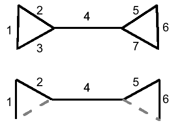
Figure 1. A graph with a total ordering of its edges and its associated $\sigma$-spanning tree.

Example 5.2.

Consider the graph with total ordering $\sigma$ of its edges depicted at the top of Fig. 1. The associated $\sigma$-spanning tree is gotten as follows. If we remove the edge labeled $7$, then the graph is connected, so we discard this edge. In $\Gamma\setminus 7$, the edge labeled 6 disconnects the graph when it is removed, so edge 6 is retained. Continuing in this fashion, the all edges but those labeled 3 and 7 are retained. This results in the spanning tree indicated by the path $1\to 2\to 4\to 5\to 6$ indicated in the bottom of Fig. 1.

Example 5.3.

A total ordering $\sigma$ is determined by a choice of non-degenerate barrier energies $W\colon\Gamma_{1}\to\mathbb{R}$, where $\alpha<\alpha^{\prime}$ if and only if $W_{\alpha}<W_{\alpha^{\prime}}$. For any such $W$ and any spanning tree $T$ we introduce the number

$$w=w(T,W)=\sum_{\alpha\in\Gamma_{1}\setminus T_{1}}W_{\alpha}\,.$$

When $W$ is understood, we sometimes write $w(T)$ for $w(T,W)$.

Proposition 5.4.

Let $W\colon\Gamma_{1}\to\mathbb{R}$ be nondegenerate. Let $\sigma$ be the ordering of edges associated with $W$, as in Example 5.3. Then, for any spanning tree $T\subset\Gamma$ with $T\neq T_{\sigma}$, there is a spanning tree $T^{\prime}\in\Gamma$, so that $w(T^{\prime},W)>w(T,W)$.

Proof.

Let $(\alpha_{1},\ldots,\alpha_{k})$ and $(\beta_{1},\ldots,\beta_{k})$ be the elements of $\Gamma_{1}\setminus(T_{\sigma})_{1}$ and $\Gamma_{1}\setminus T_{1}$, respectively, in the decreasing order with respect to $\sigma$, i.e., the barrier energies are decreasing from left to right. Let $j$ be smallest index such that

• $\alpha_{j}\neq\beta_{j}$, and

• $\alpha_{i}=\beta_{i}$ for $i<j$.

Consider the spanning subgraph $\Gamma^{\prime}\subset\Gamma$, obtained from $\Gamma$ by withdrawing the edges $\alpha_{1},\ldots,\alpha_{j-1}$, or equivalently $\beta_{1},\ldots,\beta_{j-1}$. By the definition of $T_{\sigma}$, the edge $\alpha_{j}$ is not a bridge of $\Gamma^{\prime}$ (i.e., its withdrawal does not disconnect the graph), and $W_{\beta_{i}}<W_{\alpha_{j}}$ for $i\geq j$. Let $T^{(1)}$ and $T^{(2)}$ be the two trees obtained from $T$ by withdrawing the edge $\alpha_{j}$. Then there is at least one edge, say $\beta_{s}$, among $\beta_{j},\beta_{j+1},\ldots,\beta_{k}$ that connects $T^{(1)}$ to $T^{(2)}$, since otherwise the edge $\alpha_{j}$ would be a bridge of $\Gamma$. Therefore, by replacing the edge $\beta_{s}$ with $\alpha_{j}$ in $T$ results in another spanning tree, denoted $T^{\prime}$ that obviously satisfies the condition of the proposition, since $W_{\alpha_{j}}>W_{\beta_{s}}$. ∎

Proposition 5.4 gives an immediate characterization of $\sigma$-spanning trees in terms of the function $w({-},W)$. Let $\mathcal{T}_{\Gamma}$ denote the set of spanning trees of $\Gamma$.

Corollary 5.5.

With $\sigma$ and $W$ as in Proposition 5.4, the $\sigma$-spanning tree $T_{\sigma}$ is the unique maximizer of the function $w({-},W)\colon\mathcal{T}_{\Gamma}\to\mathbb{R}$.

Remark 5.6.

One can restate the last corollary so as to depend only on $\sigma$: For $\alpha\in\Gamma_{1}$ set $W_{\sigma}(\alpha)=k$ if $\alpha$ is the $k$-th element in the partial ordering given by $\sigma$. Now define $\omega(T,\sigma):=w(T,W_{\sigma})$. Then by Corollary 5.5, $T_{\sigma}$ is the unique maximizer of $\omega({-},\sigma)\colon\mathcal{T}_{\Gamma}\to\mathbb{R}$.

Remark 5.7.

There is a useful alternative characterizing property of the $\sigma$-spanning tree $T_{\sigma}$ associated with a nondegenerate barrier function $W$: for each withdrawn edge (i.e., an edge not in $T_{\sigma}$) with $d(\alpha)=\{i,j\}$, the barrier $W_{\alpha}$ is higher than any of the barriers associated with the edges of the unique embedded path which connects $i$ to $j$ inside $T_{\sigma}$. For this reason we named $T_{\sigma}$ the minimal spanning tree of $W$ in [CKS1].

Good parameters and the weak map $\breve{q}$

Define an open subset

$$\breve{\mathcal{M}}_{\Gamma}\subset{\mathcal{M}}_{\Gamma}$$

as follows: a pair $(E,W)$ lies in $\breve{\mathcal{M}}_{\Gamma}$ if and only if one of the following conditions hold:

1. there is only one absolute minimum for $E\colon\Gamma_{0}\to\mathbb{R}$, or

2. the function $W\colon\Gamma_{1}\to\mathbb{R}$ is one-to-one, i.e., the edges are distinguished by their barrier energies. (In this instance we say that $W$ is nondegenerate.)

We call $\breve{\mathcal{M}}_{\Gamma}$ the space of good parameters.

Let $U$ be the set of $(E,W)$ satisfying the first condition and let $V$ be the set of $(E,W)$ satisfying the second. Then

$$\breve{\mathcal{M}}_{\Gamma}=U\cup V$$

where $U$ and $V$ are open. Each connected component of $U$ is defined by specifying a vertex $v\in\Gamma_{0}$, whereas each connected component of $V$ is given by specifying a total ordering $\sigma$ of $\Gamma_{1}$. Consequently, we have decompositions into connected components

$$U=\coprod_{v}U_{v}\qquad\text{ and }\qquad V=\coprod_{\sigma}V_{\sigma}\,.$$

For each vertex $v\in\Gamma_{0}$, let $B_{1/3}(v)$ be the set of points in $|\Gamma|$ which have distance $<1/3$ from $v$ in the natural metric on $|\Gamma|$ that gives every edge a length of $1$. Let $N_{v}\subset\breve{\mathcal{M}}_{\Gamma}\times|\Gamma|$ be the subspace given by $U_{v}\times B_{1/3}(v)$. Then the second factor projection

$$N_{v}\to U_{v}$$

is a homotopy equivalence (it is the cartesian product of $U_{v}$ with $B_{1/3}(v)$). Now set $N_{U}=\amalg_{v}N_{v}$. Then the projection $N_{U}\to U$ is also a homotopy equivalence. Call this projection $p_{U}$.

For a given $\sigma$, we let $N_{\sigma}\subset\breve{\mathcal{M}}_{\Gamma}\times|\Gamma|$ be the subset consisting of $V_{\sigma}\times|T_{\sigma}|(1/3)$, where $T_{\sigma}$ is the $\sigma$-spanning tree and $|T_{\sigma}|(1/3)$ consists of the points of $|\Gamma|$ whose distance to $|T_{\sigma}|$ is $<1/3$. Then the projection $N_{\sigma}\to V_{\sigma}$ is a homotopy equivalence (it is the cartesian product of $V_{\sigma}$ with a metric tree). Set $N_{V}=\amalg_{\sigma}V_{\sigma}$. Then the projection $p_{V}\colon N_{V}\to V$ is a homotopy equivalence.

Notice that $p_{U}^{-1}(U_{v}\cap N_{\sigma})\subset N_{\sigma}$. Consequently, if we set

$$N=N_{U}\cup N_{V}\,,$$

then a straightforward application of the gluing lemma [tD] shows that the first factor projection

$$p_{1}\colon N\to\breve{\mathcal{M}}_{\Gamma}$$

is a homotopy equivalence.

Definition 5.8.

For good parameters, the weak map $\breve{q}$ is given by

(11) $$\breve{\mathcal{M}}_{\Gamma}@<p_{1}<{}^{\sim}<N@>p_{2}>>|\Gamma|\,,$$

where $p_{2}$ denotes the second factor projection.

6. A weak form of the Pumping Quantization Theorem

Recall the decomposition

$$\breve{\mathcal{M}}_{\Gamma}=U\cup V$$

of the previous section, where

$$U=\coprod_{j}U_{j}\,,\qquad V=\coprod_{\sigma}V_{\sigma}\,,$$

where $j$ ranges through the elements of $\Gamma_{0}$ and $\sigma$ ranges through the set of total orderings of $\Gamma_{1}$.

Given a loop $\gamma\in L\breve{\mathcal{M}}_{\Gamma}$, it will be convenient in what follows to think of $\gamma$ as a smooth map $C\to\breve{\mathcal{M}}_{\Gamma}$, where $C$ denotes the circle of radius $1/(2\pi)$. Let $I\subset C$ be a closed arc. The contribution along $I$ to the analytical current map is then given by the integral

$$\int_{I}\mathbf{J}ds\in C_{1}(\Gamma;\mathbb{R})$$

where we parametrize $I$ with respect to arc length. That is, if $I_{1},\dots I_{k}$ is a simplicial decomposition of $C$ into closed arcs, then

$$Q_{\beta}(\gamma)=\sum_{j=1}^{k}\int_{I_{j}}\mathbf{J}ds\,.$$

Assume that $\gamma(I)\subset U$; in this instance we say $C$ is of type $U$.

Lemma 6.1.

If $I$ is of type $U$, then in the low temperature limit the contribution along $I$ to $Q_{\beta}(\gamma)$ is trivial.

Proof.

On $I$ the function $E\colon\Gamma_{0}\to\mathbb{R}$ has a unique absolute minimum $v$. As $\beta$ tends to $\infty$, the value of Boltzmann distribution $\rho^{\text{B}}$ restricted to arc $I$ tends to $v$. This is because the component of $\ell\in\Gamma_{0}$ in the Boltzmann distribution is

$$\frac{e^{-\beta E_{\ell}}}{\sum_{i}e^{-\beta E_{i}}}\,\,$$

and the latter tends to zero on if $\ell\neq v$ and one if $\ell=v$ when $E_{v}$ is the unique minimum. Consequently, as $\beta$ tends to $\infty$, the time derivative $\dot{\mathbf{\rho}}^{\text{B}}$ tends to zero on $I$ (by Lemma 3.6).

The contribution to the current of $\gamma$ along $I$ is given by the integral

$$\int_{I}A(\gamma,\dot{\mathbf{\rho}}^{\text{B}}(\gamma))ds\,,$$

(using Proposition 4.3). When $\beta$ tends to infinity, this expression tends to zero. ∎

Now consider a closed arc $I=[a,b]\subset C$ with endpoints $a,b$ such that

• $\gamma(I)\subset V$, and

• $\gamma(\partial I)\subset U$.

In this instance we say $I$ is of type $V$.

Lemma 6.2.

If $I$ is of type $V$, then in the low temperature limit the contribution along $I$ to $Q_{\beta}(\gamma)$ is an element of $C_{1}(\Gamma;\mathbb{Z})$.

Proof.

Fix a basepoint $i\in\Gamma_{0}$, $(E,W)\in{\mathcal{M}}_{\Gamma}$ and $\beta>0$. Recall from Remark 4.2 the formula

$$A^{e}(j)=\sum_{T}Q_{i}^{T,j}\varrho^{\text{B}}_{T}\qquad j\in\Gamma_{0}\,,$$

where $A^{e}\colon C_{0}(\Gamma;\mathbb{R})\to C_{1}(\Gamma;\mathbb{R})$ restricts to $A$ on $\tilde{C}_{0}(\Gamma;\mathbb{R})$. Here $\varrho^{\text{B}}_{T}$ is the $T$-component of the Boltzmann distribution for the vector space whose basis is the set of spanning trees of $\Gamma$. Recall also that the instantaneous current $\mathbf{J}(t)$ is defined as $A(\dot{\rho}^{\text{B}})$, where $\rho^{\text{B}}$ in this case denotes the Boltzmann distribution for $C_{0}(\Gamma;\mathbb{R})$. Hence, inserting $\dot{\rho}^{\text{B}}$ into the expression for $A^{e}$ gives

(12) $$\mathbf{J}(t)=\sum_{T,j}Q_{i}^{T,j}\varrho^{\text{B}}_{T}\dot{\rho}^{\text{B}}_{j}\,.$$

Recall that the average current is given by $\int_{0}^{1}\mathbf{J}(t)$. In particular, the contribution along $I$ is given by $\int_{c}^{d}\mathbf{J}(t)dt$ (where we are parametrizing $I$ with respect to arc length and the limits of integration come from the parametrization). Hence, integrating both sides of the last display, we obtain

(13) $$Q=\sum_{T,j}Q_{i}^{T,j}\int_{c}^{d}\varrho^{\text{B}}_{T}\dot{\rho}^{\text{B}}_{j}\,.$$

Since $Q_{i}^{T,j}$ is an integer valued $1$-chain, it will suffice to prove that

$$\int_{c}^{d}\varrho^{\text{B}}_{T}\dot{\rho}^{\text{B}}_{j}$$

tends to an integer as $\beta$ tends to $\infty$. Using integration by parts, we may rewrite this expression as

$$\varrho_{T}^{\text{B}}\rho_{j}^{\text{B}}|_{c}^{d}\,\,-\,\,\int_{c}^{d}\dot{\varrho}^{\text{B}}_{T}{\mathbf{\rho}}^{\text{B}}_{j}\,.$$

By Lemma 3.6, $\dot{\mathbf{\rho}}^{\text{B}}_{T}$ tends to zero as $\beta\to\infty$. Hence the constribution to the current along $I$ in the low temperature limit is determined by the value of ${\mathbf{\varrho}}_{T}^{\text{B}}{\mathbf{\rho}}_{T}^{\text{B}}|_{a}^{b}$. Since $\gamma(\partial I)\subset U$, we deduce by the argument of Lemma 6.1 that the low temperature limit of ${\mathbf{\varrho}}_{T}^{\text{B}}{\mathbf{\rho}}_{T}^{\text{B}}|_{a}^{b}$ is an integer. ∎

As an immediate corollary, we obtain a weak version of Theorem A:

Theorem 6.3 (Weak Quantization).

If $\gamma\in L\breve{M}_{\Gamma}$, then the low temperature limit $\lim_{\beta\to\infty}Q_{\beta}(\gamma)$ is defined and lies in the integral lattice $H_{1}(\Gamma;\mathbb{Z})\subset H_{1}(\Gamma;\mathbb{R})$.

7. The Discriminant Theorem and Robust Parameters

Set

$$\breve{\mathcal{D}}:={\mathcal{M}}_{\Gamma}\setminus\breve{\mathcal{M}}_{\Gamma}.$$

We will first show that the one-point compactification $\breve{\mathcal{D}}^{+}$ has the structure of a regular CW complex. By definition, $\breve{\mathcal{D}}$ is the subspace of ${\mathcal{M}}_{\Gamma}$ consisting of pairs $(E,W)$ such that $E\colon\Gamma_{0}\to\mathbb{R}$ has more than one absolute minimum and $W\colon\Gamma_{1}\to\mathbb{R}$ is not one-to-one.

Definition 7.1.

A height function for $\Gamma$ is a pair of functions

$$h_{0}:\Gamma_{0}\to\{1,2\}\,,\qquad h_{1}\colon\Gamma_{1}\to\{1,\dots,n\}\,,$$

where

• $n>0$ is an integer,

• $h_{0}^{-1}(1)$ is non-empty, and

• $h_{1}$ is surjective.

We write $h:=(h_{0},h_{1})$.

Height functions arise in the following situation.

Example 7.2.

Given $(E,W)\in\breve{\mathcal{D}}$, we write $h_{0}(i)=1$ if and only if $i$ is a minimum for $E$, and otherwise we set $h_{0}(i)=2$. We define $h_{1}\colon\Gamma_{1}\to\{1,\dots,n\}$ to be the unique surjective function characterized by

• $h_{1}(\alpha_{1})\leq h_{1}(\alpha_{2})$ if and only if $W_{\alpha_{1}}\leq W_{\alpha_{2}}$, and

• $h_{1}(\alpha_{1})=h_{1}(\alpha_{2})$ if and only if $W_{\alpha_{1}}=W_{\alpha_{2}}$.

The pair $h:=(h_{0},h_{1})$ is then a height function for $\Gamma$.

Given a height function $h=(h_{0},h_{1})$ we define

$$C(h)$$

to be the set of all $(E,W)\in\breve{\mathcal{D}}$ whose associated height function is $h$, as in Example 7.2. Then $\breve{\mathcal{D}}=\coprod_{h}C(h)$ as sets. Note that $C(h)$ is non-empty if and only if $h_{0}^{-1}(1)$ has more than one element and $h^{-1}_{1}(k)$ has more than one element for some $k$. Let $D(h)$ denote the closure of $C(h)$ in $\breve{\mathcal{D}}$.

Proposition 7.3.

Assume that $C(h)$ is non-empty. Then the one-point compactification $D(h)^{+}$ is homeomorphic to a disk of dimension $m+n$, where $m=1+|\Gamma_{0}\setminus h^{-1}_{0}(1)|$ and $n$ is as above.

Proof.

The space $C(h)$ coincides with the cartesian product $C_{0}(h)\times C_{1}(h)$, where $C_{0}(h)$ consists of those $E:\Gamma_{0}\to\mathbb{R}$ associated with $h_{0}$ and $C(h_{1})$ consists of $W:\Gamma_{0}\to\mathbb{R}$ associated with $h_{1}$. Likewise $D(h)$ coincides with the cartesian product $D(h_{0})\times D(h_{1})$.

Note that $D(h_{0})$ is canonically homeomorphic to the space $P_{m}$ consisting of $m$-tuples or real numbers

$$(x_{1},x_{2},\dots,x_{m})$$

such that $x_{1}\leq x_{k}$ for all $k>1$. The homeomorphism is given by mapping $E$ to the map $\Gamma_{0}/{\sim}\to\mathbb{R}$, where where $\sim$ denotes the equivalence relation on $\Gamma_{0}$ defined by $i\sim j$ if and only of $h_{0}(i)=1=h_{0}(j)$. As $\Gamma_{0}/{\sim}$ has cardinality one more than the number of non-minima of $E$, such functions are identified with $m$-tuples of real numbers. The operation

$$(z_{1},\dots,z_{m})\mapsto(z_{1},z_{2}+z_{1},\dots z_{m}+z_{1})$$

defines a homeomorphism to $P_{m}$ from the space of of $m$-tuples $(z_{1},\dots,z_{m})$ such that $z_{1}\in\mathbb{R}$ and $z_{k}\geq 0$ for all $k>1$. It is easy see that the one-point compactification of the latter space is homeomorphic to $D^{m}$. Hence, $D(h_{0})^{+}$ is homeomorphic to $D^{m}$.

Similarly, the space $D(h_{1})$ is canonically homeomorphic the space $Q_{n}$ consisting of $n$-tuples or real numbers

$$(x_{1},x_{2},\dots,x_{n})$$

such that $x_{1}\leq x_{2}\leq\dots x_{n}$. The operation

$$(z_{1},\dots,z_{n})\mapsto(z_{1},z_{1}+z_{2},\dots,\sum_{i=1}^{n}z_{i})$$

defines a homeomorphism to $Q_{n}$ from the space of $n$-tuples $(z_{1},\dots,z_{n})$ for which $z_{1}\in\mathbb{R}$ and $z_{i}\geq 0$ for $i>1$. The one-point compactification of the latter space is identified with $D^{n}$. Consequently, $D(h_{1})^{+}$ is homeomorphic to $D^{n}$. Finally,

$$D(h)^{+} =(D(h_{0})\times D(h_{1}))^{+}$$

$$=D(h_{0})^{+}\wedge D(h_{1})^{+}$$

$$\cong D^{m}\wedge D^{n}$$

$$=D^{m+n}\,.$$

∎

Corollary 7.4.

$\breve{\mathcal{D}}^{+}$ has the structure of a regular CW complex of dimension $d-2$, where $d$ is the cardinality of $\Gamma_{0}\amalg\Gamma_{1}$.

Remark 7.5.

With the exception of the point at $\infty$, the open cells of $\breve{\mathcal{D}}^{+}$ are given by the $C(h)$ where $h$ varies over the height functions for $\Gamma$. This is because $C(h)$ is the interior of $D(h)^{+}$.

A top dimensional cell $C(h)$ of $\breve{\mathcal{D}}^{+}$ is given by a height function $h$ in which

• $h_{0}^{-1}(1)$ has precisely two elements;

• there is a $k\leq n$ such that $h_{1}^{-1}(k)$ has precisely two elements, and if $i\neq k$ we have $h^{-1}_{1}(i)$ is a singleton for $1\leq i\leq n$.

Robust parameters

Alexander duality applied to the inclusion $\breve{\mathcal{D}}^{+}\subset\mathcal{M}_{\Gamma}^{+}=S^{d}$ yields an isomorphism

$$H^{d-2}(\breve{\mathcal{D}}^{+})\cong H_{1}(\breve{\mathcal{M}}_{\Gamma})\,.$$

Let $C^{d-2}(\breve{\mathcal{D}}^{+})$ be the cellular cochain complex of $\breve{\mathcal{D}}^{+}$ over the integers in degree $d-2$. This is the free abelian group with basis given by the set of $(d-2)$-cells of $\breve{\mathcal{D}}^{+}$. We consider the composition

(14) $$C^{d-2}(\breve{\mathcal{D}}^{+})\to H^{d-2}(\breve{\mathcal{D}}^{+})\cong H_{1}(\breve{\mathcal{M}}_{\Gamma})\overset{q_{*}}{\to}H_{1}(\Gamma;\mathbb{R})$$

where $q\colon\breve{\mathcal{M}}_{\Gamma}\to|\Gamma|$ is the weak map defined in Eq. (11) above. This homomorphism is naturally identified with a $H_{1}(\Gamma;\mathbb{R})$-valued chain

$$\phi\in C_{d-2}(\breve{\mathcal{D}}^{+};H_{1}(\Gamma;\mathbb{R}))\,,$$

and it is trivial to check that $\phi$ is a cycle. For $a\in C^{d-2}(\breve{\mathcal{D}}^{+})$, let $\langle a,\phi\rangle\in H_{1}(\Gamma;\mathbb{R})$ denote the effect of applying the homomorphism (14) to $a$.

Definition 7.6.

A $(d-2)$-cell $C(h)$ of $\breve{\mathcal{D}}^{+}$ is said to be essential if $\langle C(h),\phi\rangle\in H_{1}(\Gamma;\mathbb{R})$ is non-trivial, where we consider $C(h)$ as an element of $C^{d-2}(\breve{\mathcal{D}}^{+})$. A cell $C(h)$ of $\breve{\mathcal{D}}^{+}$ of any dimension is inessential if it is not contained in the closure of an essential $(d-2)$-cell.

Define $\check{\mathcal{D}}$ to be the closure of the union of the essential $(d-2)$-cells of $\breve{\mathcal{D}}$.

Lemma 7.7.

$\check{\mathcal{D}}^{+}$ is a subcomplex of $\breve{\mathcal{D}}^{+}$.

Proof.

It is enough to show that the union of any collection of top dimensional closed cells of $\breve{\mathcal{D}}^{+}$ forms a subcomplex. Let $D(h)^{+}$ be any closed cell of $\breve{\mathcal{D}}$. Suppose $x$ lies in the boundary of $D(h)$. Then $x$ lies in a unique (open) $j$-cell $C(h^{\prime})$. It is straightforward to check that $D(h^{\prime})\subset D(h)$. Consequently, the boundary of $D(h)^{+}$ is a union of lower dimensional cells, each of these having boundary a union of lower dimensional cells and so on. In particular, $\breve{\mathcal{D}}^{+}$ is a union of interiors of certain cells, and this union is closed. Hence it is a subcomplex. ∎

Definition 7.8.

Set

$$\check{\mathcal{M}}_{\Gamma}:={\mathcal{M}}_{\Gamma}\setminus\check{\mathcal{D}}\,.$$

Then we have an inclusion $\breve{\mathcal{M}}_{\Gamma}\subset\check{\mathcal{M}}_{\Gamma}$. We call $\check{\mathcal{M}}_{\Gamma}$ the space of robust parameters.

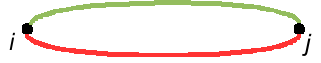
Figure 2. A two state system.

Example 7.9.

Let $\Gamma$ denote the graph displayed in Figure 2. In this case, the vector space of parameters $\mathcal{M}_{\Gamma}$ is identified with $\mathbb{R}^{4}$ and the discriminant $\breve{\mathcal{D}}$ is identified with the diagonal inclusion $\mathbb{R}^{2}\subset\mathbb{R}^{4}$ given by $(x,y)\mapsto(x,x,y,y)$. Taking the one-point compactification of this inclusion, we obtain an inclusion $S^{2}\subset S^{4}$ that is identified with $\breve{\mathcal{D}}^{+}\subset{\mathcal{M}}_{\Gamma}^{+}$. The complement of this inclusion has the homotopy type of $S^{1}$. Consequently, there is a homotopy equivalence

$$\breve{\mathcal{M}}_{\Gamma}\,\simeq S^{1}\,.$$

In fact, one can make this identification precise using the loop $\gamma$ given by the length one periodic driving protocol $\gamma(t)=(\cos 2\pi t,0,\sin 2\pi t,0)$ (one verifies this by showing that linking number of $\gamma$ with $S^{2}\subset S^{4}$ is $\pm 1$).

Consequently, the first homology group of $\breve{\mathcal{M}}_{\Gamma}$ is generated by the homology class $[\gamma]$. The effect of ${\breve{q}}_{*}\colon H_{1}(\breve{\mathcal{M}}_{\Gamma})\to H_{1}(\Gamma)$ on this loop is to produce a homology generator of $H_{1}(\Gamma;\mathbb{R})\cong\mathbb{Z}$ (see [CKS1] for details), so the weak map ${\breve{q}}\colon\breve{\mathcal{M}}_{\Gamma}\to|\Gamma|$ is a weak homotopy equivalence. In particular, the unique $2$-cell of $\breve{\mathcal{D}}^{+}\cong S^{2}$ is essential, and we infer in this instance $\check{\mathcal{M}}_{\Gamma}=\breve{\mathcal{M}}_{\Gamma}$.

Remark 7.10.

With little difficulty, Example 7.9 can be generalized to show that ${\breve{q}}_{*}\colon H_{1}(\breve{\mathcal{M}}_{\Gamma})\to H_{1}(\Gamma)$ is non-trivial whenever $\Gamma$ has non-trivial first Betti number. We omit the details.

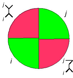
Figure 3. A two dimensional disk which meets a $(d-2)$-cell of $\breve{\mathcal{D}}$ transversely at its center. The green sectors are contained in $U$ and the red sectors are contained in $V$. In this example, the current is represented by a non-trivial cycle so the $(d-2)$-cell is essential.

The weak map $\hat{q}$

Let $C(h)$ denote a $(d-2)$-cell of $\breve{\mathcal{D}}^{+}$, and let $x\in C(h)$ be its center. We choose a small closed $2$-disk meeting $C(h)$ normally at $x$. The boundary of this disk represents a periodic driving protocol $\gamma$ in the space of good parameters. As an illustration, we have depicted such a disk in Figure 3, associated with the graph $\Gamma=$ $>\!\!\!{-}\!\!\lhd$.

If the disk is sufficiently small then it is partitioned into four regions, the interior of each either contained in $U$ or $V$, which is shown in Figure 3 as green and red respectively.

Each green sector corresponds to a vertex $i$ or $j$ of $\Gamma$, each giving a minimum for $\{E_{k}\}_{k\in\Gamma_{0}}$. Likewise, each red sector corresponds to a preferred maximal spanning tree, and these are indicated next to each such sector together with the location of the vertices $i,j$. The topological current associated with the driving protocol $\gamma$ is defined by the cycle obtained by joining together two paths connecting $i$ with $j$ (cf. §8). Each path is defined by moving along one of the spanning trees starting at $i$ and terminating at $j$ (for example, in Figure 3 one obtains the cycle $\lhd$, which is nontrivial). In particular, the cell $C(h)$ is inessential if and only if this cycle is trivial. However, even more is true: since each path used to form the cycle is embedded, it is straightforward to check that the loop in $\Gamma$ given by gluing these two paths together is null homotopic if and only if the two paths coincide. Consequently, if $\sigma$ is inessential then the weak map $\breve{q}$ extends to the space given by attaching a two cell to $\breve{\mathcal{M}}_{\Gamma}$ along $\gamma$. If we repeat this construction for every inessential $(d-2)$-cell, we obtain a space which is homotopy equivalent to the space of robust parameters $\check{\mathcal{M}}_{\Gamma}$. We have therefore shown that the weak map $\breve{q}$ admits an extension to the space of robust parameters. We denote this extension by $\hat{q}$.

However, in order to prove the Pumping Quantization Theorem, it will more convenient to give a concrete extension of the weak map $\breve{q}$ to all of $\check{\mathcal{M}}_{\Gamma}$, rather than just a model for the extension up to homotopy. This construction will be described in the next section.

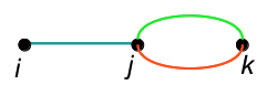
Figure 4. A graph with three vertices and three edges.

Example 7.11.

In the graph depicted by Figure 4, the edge containing vertices $i$ and $j$ is in every maximal spanning tree. Therefore, the discriminant $\breve{\mathcal{D}}$ for this graph has an inessential $4$-cell.

Definition 7.12.

A barrier resolution of a height function $h=(h_{0},h_{1})$ is a bijection $r\colon\Gamma_{1}\to\{1,\dots,|\Gamma_{1}|\}$, where $|\Gamma_{1}|$ is the cardinality of $\Gamma_{1}$, such that $h_{1}(\alpha)<h_{1}(\beta)$ implies $r(\alpha)<r(\beta)$ for all $\alpha,\beta\in\Gamma_{1}$.

A barrier resolution $r_{h}$ of $h$ enables one to associate a total ordering $\sigma_{r}$ of the set $\Gamma_{1}$. We saw in §5 how to obtain a spanning tree $T_{\sigma_{r}}$ for $\Gamma$ associated with $\sigma_{r}$. Let

$$F_{h}=\bigcap_{r}T_{\sigma_{r}}\,,$$

where the intersection is indexed over the set of barrier resolutions $r$ of $h$. Then $F_{h}$ is a forest, i.e., a (possibly empty) disjoint union of trees.

Proposition 7.13.

A cell $C(h)$ is inessential if and only if all elements of $h_{0}^{-1}(1)$ belong to the same connected component of $F_{h}$.

Proof.

Consider a cell $C(h)$ that satisfies the condition that all $i\in h_{0}^{-1}(1)$ belong to the same connected component $T_{h}$ of the forest associated with $C(h)$. Then $T_{h}$ is a tree. Consider an arbitrary top dimensional cell $C(\hat{h})$, so that $C(h)\subset D(\hat{h})$. The cell $C(\hat{h})$ is uniquely identified by two distinct vertices $i,j\in h_{0}^{-1}(1)$, and two distinct edges $\alpha$ and $\beta$ with $h_{1}(\alpha)=h_{1}(\beta)$, together with a height function $h_{1}$ of height $|\Gamma_{1}|-1$ with $\hat{h}_{1}(\alpha)=\hat{h}_{1}(\beta)$, i.e., $W_{\alpha}=W_{\beta}$ is the only edge degeneracy in $C(\hat{h})$. Then we have $\hat{h}_{0}(k)=1$ for $k=i,j$ and $\hat{h}_{0}(k)=2$, otherwise. Consider a point $(E,W)\in C(\hat{h})$, and let $\gamma_{\hat{h}}$ be a small loop that goes around $({E},{W})$ without intersecting $C(\hat{h})$, i.e., staying within the good parameter space $\breve{{\mathcal{M}}}_{\Gamma}$. Using the notation of Eq. (9), we have for the topological current

(15) $${Q}(\gamma_{\hat{h}})={Q}_{i}^{T_{\tilde{h}(\alpha)},j}-{Q}_{i}^{T_{\tilde{h}(\beta)},j}\,,$$

where $\tilde{h}_{\alpha}$ and $\tilde{h}_{\beta}$ are the two possible barrier resolutions of $\hat{h}$ with $\tilde{h}_{\alpha}>\tilde{h}_{\beta}$ and $\tilde{h}_{\alpha}<\tilde{h}_{\beta}$, respectively. Then $\tilde{h}_{\alpha}$ and $\tilde{h}_{\beta}$ are also barrier resolutions of $h$, and, therefore, $T_{h}\subset T_{\tilde{h}_{\alpha}}$ and $T_{h}\subset T_{\tilde{h}_{\beta}}$, which implies ${Q}_{i}^{T_{\tilde{h}(\alpha)},j}={Q}_{i}^{T_{h},j}={Q}_{i}^{T_{\tilde{h}(\beta)},j}$. Therefore, ${Q}(\gamma_{\hat{h}})=0$, due to Eq. (15), so that $C(h)$ is inessential.

To prove the converse, let $C(h)$ be any inessential cell. For an arbitrary pair of edges $\alpha$ and $\beta$ let $\hat{h}_{1}\colon\Gamma_{1}\to\{1,\dots,|\Gamma_{1}|-1\}$ be any surjection such that $\hat{h}_{1}(\alpha)=\hat{h}_{1}(\beta)$. Then there are two possible barrier resolutions $\tilde{h}_{\alpha}$ and $\tilde{h}_{\beta}$ of $\hat{h}$, as described above. For arbitrary distinct vertices $i$ and $j$ let $\hat{h}_{0}\colon\Gamma_{0}\to\{1,2\}$ be the function defined by

$$\hat{h}_{0}(k)=\left\{\begin{array}[]{rl}1&\mbox{ if }k=i\mbox{ or }j,\\ 2&\mbox{ otherwise.}\end{array}\right.$$

Then $\hat{h}=(\hat{h}_{0},\hat{h}_{1}$) is a height function, and $C(\hat{h})$ is top dimensional. If $C(\hat{h})$ is inessential then ${Q}(\gamma_{\hat{h}})=0$ and Eq. (15) implies that the minimal paths that connect $i$ to $j$ along the spanning trees $T_{\tilde{h}_{\alpha}}$ and $T_{\tilde{h}_{\beta}}$ are identical. Furthermore, if $D(\hat{h})\supset C(h)$, then $C(\hat{h})$ is inessential. Consequently, the set consisting of the minimal paths that connect $i$ to $j$ inside the spanning trees $T_{\tilde{h}}$ associated with all barrier resolutions $\tilde{h}$ of $h$ consists of a single element. Denote this unique path by $l_{h,ij}$. Then for any two distinct vertices $i,j\in h_{0}^{-1}(1)$ the path $l_{h,ij}$ belongs to all spanning trees $T_{\tilde{h}}$, and therefore the forest associated with $C(h)$. We infer that all vertices that belong to $h_{0}^{-1}(1)$ belong to the same connected component of the forest. ∎

8. The weak map $\check{q}$

Proposition 7.13 shows that to any inessential cell $C(h)$ one can assign, in a preferred way, a tree that contains $h_{0}^{-1}(1)$. This tree will be denoted $T_{C(h)}$ and referred to as the tree associated with the inessential cell $C(h)$. We now cover each open cell $C(h)$ with an open set $Y_{h}\supset C(h)$ that consists of all $({E},{W})\in{\mathcal{M}}_{\Gamma}$ that is characterized by the property that if $h_{0}(i)<h_{0}(j)$ and $h_{1}(\alpha)<h_{1}(\beta)$, then $E_{i}<E_{j}$ and $W_{\alpha}<W_{\beta}$, respectively, for all $i,j\in\Gamma_{0}$ and $\alpha,\beta\in\Gamma_{1}$. Setting $Y=\bigcup_{h}Y_{h}$, where the union goes over all inessential cells we obtain an open cover

(16) $$\check{{\mathcal{M}}}_{\Gamma}=U\cup V\cup Y$$

of the space of robust parameters.

For a given height function $h=(h_{0},h_{1})$ whose cell $C(h)$ is inessential, we let

$$N_{h}\subset\check{{\mathcal{M}}}_{\Gamma}\times|\Gamma|$$

be the subspace given by $Y_{h}\times|T_{C(h)}|(1/3)$, where $|T_{C(h)}|(1/3)$ is the open regular neighborhood of $|T_{C(h)}|$ given by adjoining half open subintervals of length $1/3$ that correspond to those edges not in $T_{C(h)}$ but which contain a vertex of it.

Then the projection $N_{h}\to Y_{h}$ is a homotopy equivalence. We further define $N_{Y}=\bigcup_{h}{N}_{h}$, and if we set

(17) $$\check{N}=N_{U}\cup N_{V}\cup N_{Y}\,\subset\check{{\mathcal{M}}}_{\Gamma}\times|\Gamma|\,,$$

then we have a diagram

(18) $$\check{{\mathcal{M}}}_{\Gamma}@<{p_{1}}<<\check{N}@>{p_{2}}>>|\Gamma|$$

whose arrows are given by the first and second factor projections respectively. A straightforward application of the gluing lemma which we omit shows that the projection map $p_{1}$ is a homotopy equivalence. We infer that the Eq. (18) describes a weak map which we sometimes write as

(19) $$\check{q}\colon\check{{\mathcal{M}}}_{\Gamma}\to|\Gamma|\,.$$

By construction, the restriction of $\check{q}$ to $\breve{{\mathcal{M}}}_{\Gamma}$ coincides with $\breve{q}$.

For the sake of completeness we now sketch a proof that $\check{q}$ coincides up to homotopy with the extension $\hat{q}$ of $\breve{q}$ that was described in the previous section.

Lemma 8.1.

The homotopy class of the weak map $\check{q}$ coincides with the homotopy class of the weak map $\hat{q}$ given by gluing in 2-cells.

Proof.

The result will follow from the existence of a commutative diagram

in which the vertical maps are homotopy equivalences and the left horizontal maps (denoted $p_{1}$ in each case) are also homotopy equivalences. The bottom maps labelled $p_{1}$ and $p_{2}$ comprise the weak map $\check{q}$. The top maps labelled $p_{1}$ and $p_{2}$ define the extension $\hat{q}$. The space $\hat{\mathcal{M}}_{\Gamma}$ is obtained by attaching suitable two cells to $\breve{\mathcal{M}}_{\Gamma}$; it comes equipped with a decomposition

$$\hat{\mathcal{M}}_{\Gamma}=U\cup V\cup\hat{Y}$$

where $\hat{Y}$ consists of the set of inessential $2$-cells, each which is labelled as $\hat{D}_{h}$, where $h$ ranges over height functions that define a top dimensional inessential cell. Similarly, we define $\hat{N}\subset\hat{\mathcal{M}}_{\Gamma}\times|\Gamma|$ to be the union of $N_{h}=\hat{Y}_{h}\times|T_{C(h)}|(1/3)$. Then the projections onto each factor explicitly define the extension of $\breve{q}$ described in §7.

The vertical maps in the diagram are given as follows. The homotopy equivalence $\hat{\mathcal{M}}_{\Gamma}\to\check{\mathcal{M}}_{\Gamma}$ is given by the identity on $\breve{\mathcal{M}}_{\Gamma}$ and by mapping each closed 2-cell $\check{D}_{h}$ that is attached to $\breve{\mathcal{M}}_{\Gamma}$ homeomorphically to a small closed 2-cell $\check{D}_{h}$ that intersects $C(h)$ transversely at its center (the boundary of $\check{D}_{h}$ is prescribed to having linking number +1 with $C(h)$). A similar argument which we omit defines the homotopy equivalence $\hat{N}\to\check{N}$. ∎

Remark 8.2.

For the proof of the Pumping Quantization Theorem, it will be convenient to put the open sets $U_{j}$, $V_{\sigma}$, and $Y_{h}$ on equal notational footing. This can be done by changing the notation to

$$V_{\sigma}:=Y_{h}\,,$$

where $h=(h_{0},h_{1})$ is such that $h_{0}(k)=2$ for all $k\in\Gamma_{0}$, and $h_{1}:\Gamma_{1}\to\{1,\ldots,|\Gamma_{1}|\}$ is given by $h_{1}$ is defined in the obvious sense by the total ordering $\sigma$. Similarly, we set

$$U_{j}:=Y_{h}\,,$$

where in this instance $h=(h_{0},h_{1})$ is given by $h_{0}(k)=1$ for $k=j$ and $h_{0}(k)=2$ otherwise, and $h_{1}$ is the function with constant value $1$. Note that these notational changes necessitate a more flexible notion of height function, which we will call an extended height function.

Note that the tree $T_{C(h)}$ that corresponds to $V_{\sigma}$ is just the $\sigma$-spanning tree $T_{\sigma}$, whereas $T_{C(h)}$ that corresponds to $U_{j}$ consists of the single vertex $j$ and no edges. With the above extension Eq. (17) reads $\check{N}=N_{Y}$ with $N_{Y}=\bigcup_{h}\check{N}_{h}$, where the union indexed over the set of extended height functions.

9. The Representability Theorem

Proof of Theorem B.

It is clear that $L\check{\mathcal{M}}_{\Gamma}\subset\check{L}{\mathcal{M}}_{\Gamma}$, so it suffices to prove the reverse inclusion. The proof will be by contradiction. Let $\gamma\in\check{L}{\mathcal{M}}_{\Gamma}$. The idea is to modify $\gamma$ along a small arc in such a way that the value of the current changes.

Suppose there is an $s\in[0,1]$ such that $y=\gamma(s)\in\check{\mathcal{D}}$. Then $y$ is in the closure of an essential cell. Let $\epsilon>0$ be small. Choose a point $x$ in the interior of this cell such that $|y-x|\leq\epsilon$ with respect to a choice of norm on ${\mathcal{M}}_{\Gamma}$. Let $V$ be an open neighborhood of $\gamma$ in $L{\mathcal{M}}_{\Gamma}$ on which $Q$ is well-defined and constant.

If $\epsilon$ is sufficiently small, we can construct a smooth loop $\omega\in V$ which coincides with $\gamma$ off of $(s-\epsilon,s+\epsilon)$, and inside this neighborhood $\omega$ winds once around a small disk $D$ meeting the essential cell transversely at $x$ in such a way that $D\setminus x\subset\check{\mathcal{M}}_{\Gamma}$ and $Q(\partial D)$ is nontrivial. Then topologically, $\omega$ is a loop obtained by concatenating $\gamma$ with $\partial D$. As the current $Q$ is additive, we find that $Q(\omega)=Q(\gamma)+Q(\partial D)$. Consequently, $Q(\omega)\neq Q(\gamma)$. This contradicts the assumption that $Q$ is constant on $V$. ∎

10. The Pumping Quantization and Realization Theorems

Consider a closed arc $I=[a,b]\subset C$ of our unit length circle $C$ such that $\gamma(I)\subset Y_{h}$ for some $h$. Obviously, for $c=a,b$ there is a well-defined low-temperature limit $\rho^{(c)}=\lim_{\beta\to\infty}\rho^{B}(\gamma(c);\beta)$, represented by a normalized constant function on its support ${\rm supp}(\rho^{(c)})\subset h_{0}^{-1}(1)$. We further simplify the notation by using $T_{h}=T_{C(h)}$ and chose some arbitrary base vertex $i(h)$ in the tree $T_{h}$ for each relevant height function $h$.

Lemma 10.1.

The contribution along $I$ to the current $Q_{\beta}(\gamma)$ in the low-temperature limit is given by

(20) $$\lim_{\beta\to\infty}\int_{I}{J}ds=\sum_{j\in h_{0}^{-1}(1)}{Q}_{i(h)}^{T_{h},j}\left(\rho_{j}^{(b)}-\rho_{j}^{(a)}\right).$$

Proof.

Using the explicit expression for the current based on the Kirchhoff theorem given Eq. (12) one can show

(21) $$\int_{I}{J}ds = \sum_{j\in h_{0}^{-1}(1)}{Q}_{i(h)}^{T_{h},j}\rho_{j}^{B}\sum_{T\supset T_{h}}\varrho_{T}^{B}|_{a}^{b}$$

$$- \sum_{j\in h_{0}^{-1}(1)}{Q}_{i(h)}^{T_{h},j}\int_{I}ds\rho_{j}^{B}\frac{d}{ds}\sum_{T\supset T_{h}}\varrho_{T}^{B}$$

$$+ \sum_{(j,T)\in{\mathcal{K}}_{h}}{Q}_{i(h)}^{T,j}\rho_{j}^{B}\varrho_{T}^{B}|_{a}^{b}$$

$$- \sum_{(j,T)\in{\mathcal{K}}_{h}}{Q}_{i(h)}^{T,j}\int_{I}ds\rho_{j}^{B}\dot{\varrho}_{T}^{B}\,,$$

where ${\mathcal{K}}_{h}=\left\{(j,T):h_{0}(j)=2\;{\rm or}\;T_{h}\nsubseteq T\right\}$. To derive Eq. (21) we first apply integration by parts to the explicit expression for the current, followed by representing the sum over the graph vertices $j$ and spanning trees $T$ as a sum over $(j,T)$ with $h_{0}(j)=1$ and $T\supset T_{h}$, and the remaining terms. We also make use of the fact that provided $j\in h_{0}^{-1}(1)$, which implies $j\in\left(T_{h}\right)_{0}$, and $T_{h}\subset T$, we have $Q_{i(h)}^{T,j}=Q_{i(h)}^{T_{h},j}$, i.e., the contribution to the current does not depend on the spanning tree $T$. Then Eq. (20) follows from the following properties that hold inside $Y_{h}$, and are verified directly. For $j\in h_{0}^{-1}(2)$ we have

(22) $$\lim_{\beta\to\infty}\rho_{j}^{B}=0,\;\;\;\lim_{\beta\to\infty}d\rho_{j}^{B}=0$$

and for $T\nsupseteq T_{h}$ we have

(23) $$\lim_{\beta\to\infty}\varrho_{T}^{B}=0,\;\;\;\lim_{\beta\to\infty}d\varrho_{T}^{B}=0\,.$$

Since $\sum_{T}\varrho_{T}=1$, the properties given by Eq. (23) also imply

(24) $$\lim_{\beta\to\infty}\sum_{T\supset T_{h}}\varrho_{T}^{B}=1,\;\;\;\lim_{\beta\to\infty}d\sum_{T\supset T_{h}}\varrho_{T}^{B}=0$$

Eq. (20) is obtained by applying the properties given by Eqs. (22), (23), and (24) to the integral expression of Eq. (21). ∎

Definition 10.2.

Let $\check{Q}$ be the locally constant function given by the composite

$$L\check{\mathcal{M}}_{\Gamma}@>>>H_{1}(\check{\mathcal{M}}_{\Gamma};\mathbb{Z})@>{\check{q}}_{*}>>H_{1}(\Gamma;\mathbb{Z})$$

in which the first map is defined by sending a free loop to its integer homology class.

Proof of Theorems A and E.

Let $I_{1},\ldots,I_{k}$ be a simplicial decomposition of $S^{1}$ into closed arcs, with $1,\ldots,k\in\mathbb{Z}/k$, and $I_{m}=[a_{m-1},a_{m}]$, so that $\gamma(I_{m})\subset Y_{h^{m}}$ for some set $h^{1},\ldots h^{k}$ of (extended) height functions. Applying Lemma 10.1, and more specifically Eq. (20), followed by re-grouping the terms in the sum over the arcs we obtain

(25) $$\lim_{\beta\to\infty}{Q}_{\beta}(\gamma)=\sum_{m=1}^{k}\sum_{j}\left({Q}_{i(h^{m})}^{T_{h^{m}},j}-{Q}_{i(h^{m+1})}^{T_{h^{m+1}},j}\right)\rho_{j}^{(a_{m})}\,.$$

The expression in the parenthesis on the right side of Eq. (25) does not depend on $j$. Indeed, this assertion needs only to be checked for for another vertex $j^{\prime}$ which lies in $T_{h_{m}}\cap T_{h_{m+1}}$. In this instance the unique path running from $j$ to $j^{\prime}$ which is contained in $T_{h_{m}}\cap T_{h_{m+1}}$ determines a one-chain $c$ such that ${Q}_{i(h^{m})}^{T_{h^{m}},j^{\prime}}={Q}_{i(h^{m})}^{T_{h^{m}},j}+c$ and likewise ${Q}_{i(h^{m+1})}^{T_{h^{m+1}},j^{\prime}}={Q}_{i(h^{m+1})}^{T_{h^{m+1}},j}+c$. Hence, ${Q}_{i(h^{m})}^{T_{h^{m}},j}-{Q}_{i(h^{m+1})}^{T_{h^{m+1}},j}={Q}_{i(h^{m})}^{T_{h^{m}},j^{\prime}}-{Q}_{i(h^{m+1})}^{T_{h^{m+1}},j^{\prime}}$.

If we also account for the normalization condition for $\rho^{(a_{m})}$, we can replace summation over $j$ by choosing any vertex $j_{m}\in(h_{0}^{m})^{-1}(1)\cap(h_{0}^{m+1})^{-1}(1)$ and then recast Eq.  (25) in the form

(26) $$\lim_{\beta\to\infty}{Q}_{\beta}(\gamma)\,\,=\,\,\sum_{m=1}^{k}\left({Q}_{i(h^{m})}^{T_{h^{m}},j_{m}}-{Q}_{i(h^{m+1})}^{T_{h^{m+1}},j_{m}}\right)\,.$$

The right side of Eq. (26) is clearly an integer valued one-chain, so the proof of Theorem A is complete.

We now turn to the proof of Theorem E. With respect to the above situation, consider the free loop $\ell:S^{1}\to|\Gamma|$ defined as follows: when the parameter $s\in S^{1}$ changes from the center of the arc $I_{m}$ to its end $a_{m}$, $\ell(s)$ goes from $i(h^{m})$ to $j_{m}$ along the unique minimal length path in the tree $T_{h^{m}}$. When $s$ changes from $a_{m}$ to the center of the arc $I_{m+1}$, $\ell(s)$ goes from $j_{m}$ to $i(h^{m+1})$ along the unique minimal length path in the tree $T_{h^{m+1}}$. It is easy to see that the right side of Eq. (26), considered as an element of $H_{1}(|\Gamma|)$, is the image of $\ell$ under the map $L|\Gamma|\to H_{1}(|\Gamma|)$ that associates with a free loop its corresponding homology class. On the other hand it is also easy to see that $(\gamma,\ell)\colon S^{1}\to(\check{{\mathcal{M}}}_{\Gamma}\times|\Gamma|)$ has image in $\check{N}\subset\check{{\mathcal{M}}}_{\Gamma}\times|\Gamma|$, and we infer $(\gamma,\ell)\in L\check{N}$. By a straightforward inspection of the definitions we see that the right side of Eq. (26) is given by $\check{{Q}}(\gamma)$ (as defined above in Definition 10.2), which completes the proof. ∎

11. The Chern class description

The canonical torus

Set

$$C^{i}(\Gamma;U(1)):=U(1)^{\Gamma_{i}}\qquad i=0,1\,,$$

where the right side denotes the set of functions $\Gamma_{i}\to U(1)$. The Lie group

$$G_{\Gamma}\,\,:=\,\,C^{0}(\Gamma;U(1))$$

is called the gauge group; it acts on $C^{1}(\Gamma;U(1))$. The action is defined by

$$(g\cdot f)(\alpha)=g(d_{0}(\alpha))f(\alpha)g(d_{1}(\alpha))^{-1}\,,$$

where $g\in G_{\Gamma}$ and $f\in C_{1}(\Gamma;U(1))$. Let

$$H^{1}(\Gamma;U(1))$$

denote the orbit space of this action (alternatively, let $\delta\colon C_{0}(\Gamma;U(1))\to C_{1}(\Gamma;U(1))$ be given by $\delta(g)(\alpha)=g(d_{0}(\alpha))g(d_{1}(\alpha))^{-1}$, then $H^{1}(\Gamma;U(1))$ is the cokernel of $\delta$). Then $H^{1}(\Gamma;U(1))$ is an $n$-torus where $n$ is the first Betti number of $\Gamma$ (this is the torus $S(\Gamma)$ appearing in Theorem F).

Observe that an element of $H^{1}(\Gamma;U(1))$ is represented by a function $\lambda\colon\Gamma_{1}\to U(1)$.

Lemma 11.1.

There is a preferred isomorphism

$$H^{1}(H^{1}(\Gamma;U(1));\mathbb{Z})\,\,\cong\,\,H_{1}(\Gamma;\mathbb{Z})\,.$$

Proof.

For $\alpha\in\Gamma_{1}$, let $\pi_{\alpha}\colon C^{1}(\Gamma;U(1))\to U(1)$ denote the coordinate function given by restriction to $\{\alpha\}\subset\Gamma_{1}$ (use $C^{1}(\{\alpha\};U(1))=U(1)$). The operation $\alpha\mapsto\pi^{\alpha}$ extends linearly to an isomorphism of abelian groups

$$C_{1}(\Gamma;\mathbb{Z})\cong[C^{1}(\Gamma;U(1)),U(1)]=H^{1}(C^{1}(\Gamma;U(1));\mathbb{Z})\,.$$

We also have a similar isomorphism $C_{0}(\Gamma;\mathbb{Z})\cong H^{1}(C^{0}(\Gamma;U(1));\mathbb{Z})$. With these identifications, the boundary operator $\partial\colon C_{1}(\Gamma;\mathbb{Z})\to C_{0}(\Gamma;\mathbb{Z})$ is given by restriction $\delta^{*}\colon H^{1}(C^{1}(\Gamma;U(1));\mathbb{Z})\to H^{1}(C^{0}(\Gamma;U(1));\mathbb{Z})$. Hence $H_{1}(\Gamma;\mathbb{Z})$ is identified with the kernel of $\delta^{*}$. But the inclusion $H^{1}(H^{1}(\Gamma;U(1));\mathbb{Z})\subset\text{\rm ker}(\delta^{*})$ is clearly an isomorphism. ∎

A combinatorially defined line bundle

We refer the reader to discussion of §8, especially Remark 8.2. Recall that

$$\check{\mathcal{M}}_{\Gamma}=\bigcup_{h}Y_{h}$$

is a covering by open sets where $h=(h_{0},h_{1})$ ranges over extended height functions. Associated with $Y_{h}$ one has a tree $T_{h}:=T_{C(h)}$ such that $h_{0}^{-1}(1)\subset T_{C(h)}$. Fix a basepoint vertex $i$ for $T_{h}$ (cf. Lemma 10.1)

For $(E,W)\in Y_{h}$ and $\lambda\in C^{1}(\Gamma;U(1))$, we associate a complex line in $\mathbb{C}^{n}$, where $n$ is the cardinality of $\Gamma_{1}$. For any vertex $j$ of the tree $T_{h}$, we have a minimal path $P_{i}^{T_{h},j}$ from $i$ to $j$ which is contained in $T$; this path defines the integer value 1-chain $Q_{i}^{T_{h},j}$ (cf. Remark 4.2).

Let $\mathbb{C}[\Gamma_{0}]$ denote the complex vector space with basis $\Gamma_{0}$. Then we obtain a non-zero vector

(27) $$v=v(h,E,W,\lambda):=\sum_{j\in(T_{h})_{0}}(e^{-\beta E_{j}}\prod_{\alpha\in P_{i}^{T_{h},j}}\lambda^{s(\alpha)}_{\alpha})j\,\,\in\,\,\mathbb{C}[\Gamma_{0}]$$

where $s(\alpha)=\pm 1$ according as to whether the direction of the path coincides with the orientation of $\alpha$ (this sign coincides with the coefficient appearing of $\alpha$ in $Q_{i}^{T_{h},j}$).

Let $\mathbb{C}v\subset\mathbb{C}[\Gamma_{0}]$ denote the complex line spanned by this vector.

Lemma 11.2.

If we choose a different basepoint vertex the complex line $\mathbb{C}v$ remains unchanged.

Proof.

The amalgamation of the minimal length paths $P_{i}^{T_{h},i^{\prime}}$ and $P_{i^{\prime}}^{T_{h},j}$ produces a new path $P_{i}^{T_{h},i^{\prime}}P_{i^{\prime}}^{T_{h},j}$ from $i$ to $j$. If this path is minimal, then it is $P_{i}^{T_{h},j}$ and clearly, we have

$$\prod_{\alpha\in P_{i}^{T_{h},j}}\lambda^{s(\alpha)}_{\alpha}=(\prod_{\alpha\in P_{i}^{T_{h},i^{\prime}}}\lambda^{s(\alpha)}_{\alpha})(\prod_{\alpha\in P_{i^{\prime}}^{T_{h},j}}\lambda^{s(\alpha)}_{\alpha})\,.$$

If the amalgamated path isn’t minimal, then this formula still holds because the factors corresponding to indices occurring more than once cancel. This gives independence with respect to the basepoint vertex, as the first factor on the right is independent of $j$. ∎

For fixed $h$ the assignment $(E,W,\lambda)\mapsto{\mathbb{C}}v(h,E,W,\lambda)$ describes a line bundle $\tilde{\xi}_{h}$ over $C^{1}(\Gamma;U(1))\times Y_{h}$. In fact, it is straightforward to check that $\tilde{\xi}_{h}$ is trivializable. We now use the clutching construction to glue these line bundles together as $h$ varies. This will produce a line bundle over $\tilde{\xi}$ over $C^{1}(\Gamma;U(1))\times\check{\mathcal{M}}_{\Gamma}$. To check this, it suffices to establish the following.

Lemma 11.3.

Given height functions $h$ and $h^{\prime}$, let

$$a\colon C^{1}(\Gamma;U(1))\times(Y_{h}\cap Y_{h^{\prime}})\to C^{1}(\Gamma;U(1))\times Y_{h}$$

and

$$b\colon C^{1}(\Gamma;U(1))\times(Y_{h}\cap Y_{h^{\prime}})\to C^{1}(\Gamma;U(1))\times Y_{h^{\prime}}$$

denote the inclusions. Then there is an isomorphism of line bundles $\phi_{ab}\colon b^{*}\tilde{\xi}_{h^{\prime}}@>\cong>>a^{*}{\tilde{\xi}}_{h}$. Furthermore, this isomorphism satisfies the cocycle condition $\phi_{ac}=\phi_{ab}\phi_{bc}$.

Proof.

Associated with $(\lambda,E,W)\in C^{1}(\Gamma;U(1))\times Y_{h}$ and a basepoint vertex $i$ for $T_{h}\cap T_{h^{\prime}}$, we have a non-zero vector $v$ which is defined by Eq. (27). To indicate the dependence of this vector on $h$, let us redenote it by $v_{h}$. Similarly, for $(\lambda,E,W)\in C^{1}(\Gamma;U(1))\times Y_{h^{\prime}}$ we have $v_{h^{\prime}}$. Then define $\phi_{ab}(z\cdot v_{h^{\prime}}):=z\cdot v_{h}$. The cocycle condition is then immediate. ∎

Let the gauge group $G_{\Gamma}$ act diagonally $C^{1}(\Gamma;U(1))\times\check{\mathcal{M}}_{\Gamma}$ (where the action on the second factor is trivial). Then $G_{\Gamma}$ also acts in an evident way on the total space $E(\tilde{\xi})$ of the line bundle $\tilde{\xi}$ equipping it with the structure of a $G_{\Gamma}$-equivariant line bundle. Taking orbit spaces defines a line bundle $\xi$ over $H^{1}(\Gamma;U(1))\times\check{{\mathcal{M}}}_{\Gamma}$. If $\pi\colon C^{1}(\Gamma;U(1))\to H^{1}(\Gamma;U(1))$ is the quotient map, then $\tilde{\xi}$ is given by the base change of $\xi$ along

$$\pi\times\text{id}\colon C^{1}(\Gamma;U(1))\times\check{{\mathcal{M}}}_{\Gamma}\to H^{1}(\Gamma;(U(1))\times\check{{\mathcal{M}}}_{\Gamma}\,.$$

Naturality of Chern classes gives a commutative diagram

(28)

Here we have used the preferred isomorphism $H^{1}(H^{1}(\Gamma;U(1));\mathbb{Z})=H_{1}(\Gamma;\mathbb{Z})$ of Lemma 11.1 as well as a similarly constructed identification $H^{1}(C^{1}(\Gamma;U(1));\mathbb{Z})=C_{1}(\Gamma;\mathbb{Z})$. With respect to these identifications, $\pi^{*}$, which is the homomorphism induced by $\pi$ on first integer cohomology, is just the canonical inclusion $H_{1}(\Gamma;\mathbb{Z})\subset C_{1}(\Gamma;\mathbb{Z})$.

Theorem 11.4.

The homomorphism $c_{1}(\xi)/$ coincides with ${\check{q}}_{*}$.

In order to prove Theorem 11.4 we digress to explain how holonomy relates to the homomorphism given by slant product with the first Chern class. If $\xi$ is a complex line bundle over a connected space $B$ and structure group $U(1)$, we have the holonomy map

(29) $$h_{\xi}\colon LB\to U(1)\,.$$

In fact, $h_{\xi}$ can be chosen in such a way that if we choose a basepoint of $B$ and restrict $h_{\xi}$ to the based loop space $\Omega B$, we can deloop to a map $B\to BU(1)={\mathbb{C}}P^{\infty}$ that classifies the bundle $\xi$ and hence the Chern class $c_{1}(\xi)$. Consequently, if we choose $h_{\xi}$ in this way, it determines the Chern class.

Now suppose $B=X\times Y$. Then we can restrict $h_{\xi}$ to the subspace $X\times LY\subset LX\times LY=L(X\times Y)$ and take the adjoint to obtain a map

$$LY\to F(X,U(1))\,,$$

where $F(X,U(1))$ is the function space of maps from $X$ to $U(1)$. Then the diagram

(30)

commutes, where the left vertical map sends a loop to its homology class and the right vertical map sends a function to its homotopy class considered as an element of $H^{1}(X;\mathbb{Z})=[X,U(1)]$.

Proof of Theorem 11.4.

By Eq. (28) it suffices to show that $c_{1}(\tilde{\xi})/$ coincides with the homomorphism

$$H_{1}(\check{\mathcal{M}}_{\Gamma};\mathbb{Z})@>{\check{q}}_{*}>>H_{1}(\Gamma;\mathbb{Z})@>\pi^{*}>>C_{1}(\Gamma;\mathbb{Z})\,.$$

Suppose we are given $(\lambda,\gamma)\in C^{1}(\Gamma;U(1))\times L\check{\mathcal{M}}_{\Gamma}$. As done previously, we partition $S^{1}$ into closed arcs $[a_{k},a_{k+1}]$ for $0\leq k\leq n$ with $a_{n+1}\equiv a_{0}$, such that the projection of such an arc into $\check{\mathcal{M}}_{\Gamma}$ is contained in a neighborhood of type $Y_{h_{k-1}}$. Choose a basepoint vertex $i_{k}$ lying in the intersection $T_{k}\cap T_{k+1}$, where $T_{k}$ denotes the tree associated with $Y_{h_{k}}$ . Then we have a minimal length path $P_{i_{k}}^{T_{k},i_{k+1}}$ from $i_{k}$ to $i_{k+1}$ and the product

(31) $$\prod_{k=0}^{n}\prod_{\alpha\in P_{i_{k}}^{T_{k},i_{k+1}}}\lambda^{s(\alpha)}_{\alpha}\in U(1)$$

describes a map $C^{1}(\Gamma;U(1))\to U(1)$ that gives the holonomy around $\gamma$ (here we are using Lemmas 11.2 and 11.3).

In the special instance of $\lambda\in C^{1}(\Gamma;U(1))$ which is identically $1$ except for a single edge $\alpha$, the value of the map $C^{1}(\Gamma;U(1))\to U(1)$ at $\lambda$ is given by $\lambda_{\alpha}^{q}$ where $q$ represents the net number of times $\alpha$ is traversed, with orientation taken into account. Consequently, if we identify $H^{1}(C^{1}(\Gamma;U(1));\mathbb{Z})$ with $C_{1}(\Gamma;\mathbb{Z})$, then $\lambda_{\alpha}^{q}$ is identified with the chain $q\alpha$. It follows that the map $C^{1}(\Gamma;U(1))\to U(1)$ defined by Eq. (31) corresponds to the integer cycle in $C_{1}(\Gamma;\mathbb{Z})$ given by

(32) $$\sum_{k=0}^{n}\sum_{\alpha\in P_{i_{k}}^{T_{k},i_{k+1}}}s(\alpha)\alpha\,\,:=\,\,\sum_{k=0}^{n}Q_{i_{k}}^{T_{k},i_{k+1}}\,.$$

On the other hand, the paths $P_{i_{k}}^{T_{k},i_{k+1}}$ describe a lift of $\gamma\colon S^{1}\to\check{\mathcal{M}}_{\Gamma}$ through the space $\check{N}$ appearing Eq. (17) (roughly, one defines the lift by mapping the midpoint $a^{\prime}_{k}$ of the arc $[a_{k},a_{k+1}]$ to the point $(\gamma(a^{\prime}_{k}),i_{k})$ and uses $P_{i_{k}}^{T_{k},i_{k+1}}$ to connect these points). Then application of the projection map $p_{2}\colon\check{N}\to|\Gamma|$ to the given lift produces a map $S^{1}\to|\Gamma|$ that represents $\check{q}_{*}([\gamma])\in H_{1}(\Gamma;\mathbb{Z})\subset C_{1}(\Gamma;\mathbb{Z})$. From this description it is straightforward to check that $\check{q}_{*}([\gamma])$ coincides with the element defined by Eq. (32) (cf. Eq. (9)). ∎

12. The ground state bundle: a conjecture

By coupling the master operator with elements of the torus $H^{1}(\Gamma;U(1))$ one can extend the master operator to a self-adjoint operator over the complex numbers. This extension is called the twisted master operator; its eigenvalues are real and non-positive. The eigenspace associated with the maximum non-zero eigenvalue is called the ground state. One may use the twisted master operator to define another weak complex line bundle $\eta$, this time over $H^{1}(\Gamma;U(1))\times\tilde{\mathcal{M}}_{\Gamma}$, where $\tilde{\mathcal{M}}_{\Gamma}\subset{\mathcal{M}}_{\Gamma}$ is characterized by the condition that the ground state at each point is non-degenerate, meaning that it has rank one. Then roughly, $\eta$ is defined by taking the ground state at each point of the base. We call this the ground state bundle. Arguments from physics suggest that the ground state bundle is equivalent to the weak complex line bundle $\xi$ that was defined in the previous section. In what follows we will formulate this idea as a pair of conjectures.

The twisted master operator

The twisted master operator, defined below, is a smooth map

$$\bar{H}\colon C^{1}(\Gamma;U(1))\times\mathcal{M}_{\Gamma}\to\operatorname{end}_{\mathbb{C}}(C_{0}(X;\mathbb{C}))\,,$$

where $C_{0}(X;\mathbb{C})$ is the complex vector space with basis $\Gamma_{0}$. It extends the master operator in the sense that

$$\bar{H}(1,\beta,E,W)=H(\beta,E,W)$$

where $1\in C^{1}(\Gamma;U(1))$ is the function with constant value $1\in U(1)$ and where we are interpreting the right side of this identity using extension of scalars.

For $\lambda\in C^{1}(\Gamma;U(1))$, let $\hat{\lambda}\colon C_{1}(\Gamma;\mathbb{C})\to C_{1}(\Gamma;\mathbb{C})$ be given by rescaling each basis element $\alpha$ by $\lambda(\alpha)\alpha$. Then

$$\bar{H}(\lambda,\beta,E,W):=-\partial\hat{g}^{-1}\hat{\lambda}\partial^{*}\hat{\kappa}\,.$$

It is clear from the definition that $\bar{H}$ is self-adjoint. In particular, its eigenvalues are all real.

Let the gauge group $G_{\Gamma}$ act on $\operatorname{end}_{\mathbb{C}}(C_{0}(X;\mathbb{C}))$ via conjugation and trivially on $\mathcal{M}_{\Gamma}$. The following is then a formal consequence of the definitions.

Lemma 12.1 (Gauge Symmetry).

The twisted master operator is $G_{\Gamma}$-equivariant, i.e., for $h\in G_{\Gamma}$, we have

$$\bar{H}(h\cdot\lambda,\beta,E,W)=h\cdot\bar{H}(\lambda,\beta,E,W)\,.$$

In particular, for each $(E,W)\in\mathcal{M}_{\Gamma}$, the spectrum of $H(\beta,E,W)=\bar{H}(1,\beta,E,W)$ is invariant with respect to the action of the gauge group.

Definition 12.2.

Let $A\colon V\to V$ be a self-adjoint linear transformation of a finite dimensional complex vector space $V$, all of whose eigenvalues are non-positive. Then the ground state $L$ is the eigenspace for maximal eigenvalue of $A$. We say that $A$ has nondegenerate its ground state $L$ has rank one.

An analytically defined weak line bundle

Define an open subset

$$\tilde{\mathcal{M}}_{\Gamma}\subset\mathbb{R}_{+}\times\mathcal{M}_{\Gamma}$$

to be the set of those $(\beta_{0},E,W)$ such that for every $\lambda\in C^{1}(\Gamma;U(1))$ and every $\beta\geq\beta_{0}$, the twisted master operator

$$\bar{H}(\lambda,\beta,E,W)\colon C_{0}(\Gamma;\mathbb{C})\to C_{0}(\Gamma;\mathbb{C})$$

has a non-degenerate ground state.

For $(\lambda,\beta_{0},E,W)\in C^{1}(\Gamma;U(1))\times\tilde{\mathcal{M}}_{\Gamma}$, let us denote the ground state of the twisted master operator by $\mathbb{L}(\beta_{0},\lambda,E,W)$; it is a complex line in $C_{0}(\Gamma;\mathbb{C})$. Consider

$$E=\{(\lambda,\beta_{0},E,W,v)|v\in\mathbb{L}(\beta_{0},\lambda,E,W)\}$$

which is topologized as a subspace of $C^{1}(\Gamma;U(1))\times\tilde{\mathcal{M}}_{\Gamma}\times C_{0}(\Gamma;\mathbb{C})$. Then we have an evident projection

$$p\colon E\to C^{1}(\Gamma;U(1))\times\tilde{\mathcal{M}}_{\Gamma}\,.$$

Lemma 12.3.

The map $p$ is a smooth complex line bundle projection.

Proof.

Let $V=C_{0}(\Gamma;\mathbb{C})$ and let $L^{1}(V,V)$ denote the space consisting of complex linear self-maps of $V$ having corank one. Then $L^{1}(V,V)$ is a smooth manifold of real dimension $2|\Gamma_{0}|^{2}-2$ (see [GG, prop. 5.3]). The operation which sends a complex linear self-map to its null space defines a smooth map

$$L^{1}(V,V)@>\text{ker}>>\mathbb{P}^{1}(V)$$

whose target is the projective space of complex lines in $V$. The composition

$$C^{1}(\Gamma;\mathbb{C})\times\tilde{\mathcal{M}}_{\Gamma}@>\bar{H}>>L^{1}(V,V)@>\text{ker}>>\mathbb{P}^{1}(V)$$

is therefore smooth and the pullback of the tautological line bundle over $\mathbb{P}^{1}(V)$ gives the projection $p$. ∎

Let $\pi\colon\tilde{\mathcal{M}}_{\Gamma}\to{\mathcal{M}}_{\Gamma}$ be given by the projection $(\beta_{0},E,W)\mapsto(E,W)$.

Conjecture 12.4.

The image of $\pi$ is $\check{\mathcal{M}}_{\Gamma}$, and $\pi\colon\tilde{\mathcal{M}}_{\Gamma}\to\check{\mathcal{M}}_{\Gamma}$ is a weak homotopy equivalence.

Let $\tilde{\eta}$ be the complex line bundle defined by Lemma 12.3. The gauge group $G_{\Gamma}$ acts on both the total and base spaces making $\tilde{\eta}$ into a $G_{\Gamma}$-equivariant complex line bundle. Taking orbits, we obtain a complex line bundle $\eta$ over $H^{1}(\Gamma;U(1))\times\tilde{\mathcal{M}}_{\Gamma}$.

Let $h\colon H^{1}(\Gamma;U(1))\times\tilde{\mathcal{M}}_{\Gamma}\to H^{1}(\Gamma;U(1))\times\check{\mathcal{M}}_{\Gamma}$ be given by $\text{id}\times\pi$. Then using Lemma 12.4, the pair $(\eta,h)$ is a weak complex line bundle over $H^{1}(\Gamma;U(1))\times\check{\mathcal{M}}_{\Gamma}$.

Then slant product with the first Chern class of $\eta$ gives a homomorphism

$$c_{1}(\eta)/\colon H_{1}(\check{\mathcal{M}}_{\Gamma};\mathbb{Z})\to H_{1}(\Gamma;\mathbb{Z})\,,$$

where we have implicitly used the identification $H_{1}(\check{\mathcal{M}}_{\Gamma};\mathbb{Z})\cong H_{1}(\tilde{\mathcal{M}}_{\Gamma};\mathbb{Z})$ of Lemma 12.4 and also the identification $H^{1}(H^{1}(\Gamma;U(1));\mathbb{Z})\cong H_{1}(\Gamma;\mathbb{Z})$ of Lemma 11.1.

Conjecture 12.5.

The homomorphisms $c_{1}(\eta)/$ and $c_{1}(\xi)/$ coincide.

13. Appendix: an adiabatic theorem

Here we formulate and prove an adiabatic theorem for periodic driving. Roughly, it states that for slow enough driving a periodic solution of the master equation exists and is unique, and furthermore, in the adiabatic limit this solution will tend to the Boltzmann distribution taken at the associated normalized driving protocol.

Let us introduce the evolution operator $U(t,t_{0})=U(t,t_{0};H,\tau_{D})$ for $0\leq t_{0}\leq t\leq 1$, which is the unique solution to the initial value problem

$$\frac{d}{dt}U(t,t_{0})=\tau_{D}U(t,t_{0})H(\gamma(t)),\qquad U(t_{0},t_{0})=I\,,$$

where $I$ denotes the identity operator. We remark that $U(t,t_{0})$ is also called the path-ordered exponential and is sometimes expressed in the notation

$$\hat{T}\exp(\tau_{D}\int_{t_{0}}^{t}dt^{\prime}H(\gamma(t^{\prime})))$$

(cf. [L]).

Then it is elementary to show that the master equation

$$\dot{\mathbf{p}}(t)=\tau_{D}H(\gamma(t)){\mathbf{p}}(t)$$

has formal solution

$$\mathbf{p}(t)=U(t,0)\mathbf{p}(0)\,.$$

Proposition 13.1.

Let $(\tau_{D},\gamma)$ be a periodic driving protocol. Then there is positive real number $\tau_{0}$ such that if $\tau_{D}\geq\tau_{0}$, then there is a unique periodic solution $\rho(t)$ to the master equation, i.e., $\rho(0)=\rho(1)$.

Proof.

We shall use abbreviated notation and write $\rho^{\text{\rm B}}(t)$ in place of $\rho^{\text{\rm B}}(\gamma(t))$. For any solution to the master equation ${\mathbf{p}}(t)$, set

$$\xi(t):=\mathbf{\rho}^{\text{\rm B}}(t)-{\mathbf{p}}(t)\,.$$

Then $\xi\colon[0,1]\to\tilde{C}_{0}(\Gamma;\mathbb{R})$ is a family of reduced population vectors. Furthermore, $\xi(t)$ is periodic if and only ${\mathbf{p}}(t)$ is, and

(33) $${\mathbf{p}}(t)=\mathbf{\rho}^{\text{\rm B}}(t)+\xi(t)\,.$$

Inserting Eq. (33) expression into the master equation and using the fact that the Boltzmann distribution lies in the null space of the master operator, we obtain the first order linear differential equation in $\xi$,

(34) $$\dot{\xi}(t)-\tau_{D}H(t)\xi(t)=-\dot{\rho}^{\text{\rm B}}(t)\,,$$

where $H(t)$ is shorthand for $H(\gamma(t))$.

Applying $U(1,t)$ to Eq. (34) we get

$$U(1,t)\dot{\xi}-U(1,t)\tau_{D}H\xi=-U(1,t)\dot{\rho}^{\text{\rm B}}\,.$$

Notice that the left side of the last display is just $d/dt(U(1,t)\xi)$. Integrating both sides we obtain

$$U(1,t)\xi(t)=-\int_{0}^{t}U(1,t^{\prime})\dot{\rho}^{\text{\rm B}}\,dt^{\prime}+C\,.$$

Setting $t=0$ we see that $U(1,0)\xi(0)=C$. Evaluating at $t=1$ and using the fact that $U(1,1)=I$ yields

$$\xi(1)-U(1,0)\xi(0)=-\int_{0}^{1}U(1,t^{\prime})\dot{\rho}^{\text{\rm B}}\,dt^{\prime}\,.$$

Consequently, $\xi(0)=\xi(1)$ if and only if

(35) $$(I-U(1,0))\xi(0)=-\int_{0}^{1}U(1,t^{\prime})\dot{\rho}^{\text{\rm B}}\,dt^{\prime}\,.$$

It is therefore sufficient to show that the operator $I-U(1,0)$ is invertible, when considered as an operator acting on the invariant subspace $\tilde{C}_{0}(\Gamma;\mathbb{R})$, provided $\tau_{D}$ is sufficiently large.

Let $\lambda$ and $c$ be the constants obtained in Lemma 13.2 below. If we set $\tau_{0}:=(1/\lambda)\ln(2c)$, then we have $\|U(1,0)\|<1/2$. It follows that $I-U(1,0)$ is invertible on $\tilde{C}_{0}(\Gamma;\mathbb{R})$. ∎

The last part of the proof of Proposition 13.1 rested on an estimate that appears below. To formulate it we use the norm on $\tilde{C}_{0}(\Gamma;\mathbb{R})$ given by $\|\xi\|=\sqrt{\langle\xi,\xi\rangle}$ where the inner product is the one induced by the standard inner product on $C_{0}(\Gamma;\mathbb{R})$. If $A$ is an operator on $\tilde{C}_{0}(\Gamma;\mathbb{R})$ then we define $\|A\|:=\sup_{\xi\neq 0}\|A\xi\|\|\xi\|^{-1}=\sup_{\xi=1}\|A\xi\|.$

Lemma 13.2.

For a periodic driving protocol $(\tau_{D},\gamma)$, there are positive constants $\lambda$ and $c$ such that for all $t,t_{0}\in[0,1]$ we have

$$\|U(t,t_{0})\|<ce^{-\lambda\tau_{D}(t-t_{0})}\,.$$

Proof.

Consider the time-dependent inner product $\kappa_{t}=\kappa(\gamma(t))$ in $\tilde{C}_{0}(\Gamma;\mathbb{R})$, defined by $\kappa_{t}(\xi,\eta)=\sum_{j\in\Gamma_{0}}e^{\beta E_{j}(t)}\xi_{j}\eta_{j}$ (the is just $\langle{\xi},{\eta}\rangle_{\hat{\kappa}_{t}}$ in the notation of Remark 3.3). Then for all $t$ the operator $H(t)=H(\gamma(t))$, when considered as acting on $\tilde{C}_{0}(\Gamma;\mathbb{R})$, is self-adjoint with respect to the inner product $\kappa_{t}$ and its spectrum is strictly negative.

Set $\lambda:=-\sup_{t\in[0,1]}\sigma(H(t))$, where $\sigma(T)$ denotes the spectrum of a linear operator $T$. Then $\lambda>0$, and the spectrum of the operator ${H}_{0}(t)={H}(t)+\lambda I$ is non-negative for all $t$. Let $U_{0}(t,t_{0})$ be the corresponding evolution operator. Then $U(t,t_{0})=e^{-\lambda\tau_{D}(t-t_{0})}U_{0}(t,t_{0})$. Hence, $\|{U}(t,t_{0})\|=e^{-\lambda\tau_{D}(t-t_{0})}\|{U}_{0}(t,t_{0})\|$. So all we need to prove is that $\|{U}_{0}(t,t_{0})\|$ is uniformly bounded.

Let $\eta(t)$ be the solution of the master equation $\dot{\eta}(t)=\tau_{D}H_{0}(t)\eta(t)$ with the initial condition $\eta(t_{0})=\xi$. We then have

(36) $$\frac{d}{dt}\kappa_{t}(\eta(t),\eta(t)) = \dot{\kappa}_{t}(\eta(t),\eta(t))+2\tau_{D}\kappa_{t}({H}_{0}(t)\eta(t),\eta(t))$$

$$\leq \dot{\kappa}_{t}(\eta(t),\eta(t)),$$

since for all $t$ we have $\kappa_{t}({H}_{0}(t)\eta(t),\eta(t))\leq 0$.

Since $\eta(t)\neq 0$ provided $\eta(t_{0})=\xi\neq 0$, we infer that $\kappa_{t}(\eta(t),\eta(t))>0$ for all $t$. By compactness, $\|\kappa_{t}\|$ is bounded below, and since $\|\dot{\kappa}_{t}\|$ is bounded above, we infer that there is a constant $A>0$, so that $\dot{\kappa}_{t}(\eta(t),\eta(t))(\kappa_{t}(\eta(t),\eta(t)))^{-1}<A$. Combined with Eq. (36) this implies $(d/dt)\ln\kappa_{t}(\eta(t),\eta(t))<A$, and further implies the uniform bound

(37) $$\frac{\kappa_{t}({U}_{0}(t,t_{0})\xi,{U}_{0}(t,t_{0})\xi)}{\kappa_{t_{0}}(\xi,\xi)}=\frac{\kappa_{t}(\eta(t),\eta(t))}{\kappa_{t_{0}}(\eta(t_{0}),\eta(t_{0}))}<e^{A(t-t_{0})}.$$

The uniform bound provided by Eq. (37) implies the uniform bound

(38) $$\frac{\langle{U}_{0}(t,t_{0})\xi,{U}_{0}(t,t_{0})\xi\rangle}{\langle\xi,\xi\rangle}<B^{2},$$

with respect to the standard inner product for some $B>0$, which immediately implies the uniform bound $\|{U}_{0}(t,t_{0})\|<B$. ∎∎

Corollary 13.3 (Adiabatic Theorem, cf. [vK, V.3]).

Let $(\tau_{D},\gamma)$ be a periodic driving protocol, with $\tau_{D}$ sufficiently large. If $\mathbf{\rho}(t)$ denotes the periodic solution of the master equation, then

$$\mathbf{\rho}^{\text{\rm B}}(\gamma(t))=\lim_{\tau_{D}\to\infty}\mathbf{\rho}(t)\,.$$

Proof.

It is enough to show that $\lim_{\tau_{D}\to\infty}\xi(t)=0$ where $\xi(t)$ is as in the proof of Proposition 13.1. We first show that $\lim_{\tau_{D}\to\infty}\xi(0)=0$.

To see this, start with the estimate

$$\|\int_{0}^{t}U(t,t^{\prime})\dot{\rho}^{\text{\rm B}}(t^{\prime})\,dt^{\prime}\| \leq\int_{0}^{t}\|U(t,t^{\prime})\|\|\dot{\rho}^{\text{\rm B}}(t^{\prime})\|\,dt^{\prime}$$

$$\leq c\sup_{t^{\prime}\in[0,1]}\|\dot{\rho}^{\text{\rm B}}(t^{\prime})\|\int_{0}^{1}e^{-\lambda\tau_{D}(1-t)}\,dt$$

$$<\frac{\alpha c}{\lambda\tau_{D}}\,,$$

where $\alpha=\sup_{t^{\prime}\in[0,1]}\|\dot{\rho}^{\text{\rm B}}(t^{\prime})\|$. Recalling that $\|U(1,0)\|<1/2$, we have $\|(I-U(1,0))^{-1}\|<2$. Consequently,

$$\|\xi(0)\| =\|(I-U(1,0))^{-1}\int_{0}^{1}U(1,t^{\prime})\dot{\rho}^{\text{\rm B}}\,dt^{\prime}\|$$

$$\leq\|(I-U(1,0))^{-1}\|\|\int_{0}^{1}U(1,t^{\prime})\dot{\rho}^{\text{\rm B}}\,dt^{\prime}\|$$

$$<\frac{2\alpha c}{\lambda\tau_{D}}$$

Therefore, $\lim_{\tau_{D}\to\infty}\xi(0)=0$.

The proof that $\lim_{\tau_{D}\to\infty}\xi(t_{0})=0$ for any $t_{0}\in[0,1]$ is similar, using a suitable modification of the above estimate with $t_{0}$ in place of $0$ and Lemma 13.2) to give a similar bound for $\|\xi(t_{0})\|$ (we omit the details). ∎

References

- [B] Bollobás, Béla: Modern graph theory. Graduate Texts in Mathematics, 184. Springer-Verlag, New York, 1998.
- [CKS1] Chernyak, V.Y., Klein J.R., Sinitsyn, N.A.: Quantization of fluctuating currents in stochastic networks, to appear in J. Chem. Physics.
- [CKS2] Chernyak, V.Y., Klein J.R., Sinitsyn, N.A.: Quantization of fluctuating currents in stochastic networks, II: full counting statistics, to appear in J. Chem. Physics.
- [GG] Golubitsky, M., Guillemin, V.: Stable mappings and their singularities. Graduate Texts in Mathematics, 14. Springer-Verlag, New York-Heidelberg, 1973.
- [H] Hatcher, A.: Algebraic Topology. Cambridge University Press, Cambridge, 2002.
- [HJ] Horowitz, J., Jarzynski C.: Exact formula for currents in strongly pumped diffusion systems, J. Stat. Phys. 136 (2009), 917 -925
- [L] Lam, C.S.: Decomposition of time-ordered products and path-ordered exponentials, J. Math. Phys. 39, (1998) 5543–5558
- [NR] Nerode, A., Shank H.: An algebraic proof of Kirchhoff’s network theorem, Amer. Math. Monthly 68, (1961) 244- 247
- [tD] tom Dieck, T.: Partitions of unity in homotopy theory, Composito Math. 23 (1971), 159- 167
- [vK] van Kampen, N.G.: Stochastic processes in physics and chemistry, 3rd ed. North-Holland Personal Library, Elsevier, Amsterdam, 2007