Mathematical Modeling of Competitive Group Recommendation Systems with Application to Peer Review Systems

Abstract

In this paper, we present a mathematical model to capture various factors which may influence the accuracy of a competitive group recommendation system. We apply this model to peer review systems, i.e., conference or research grants review, which is an essential component in our scientific community. We explore number of important questions, i.e., how will the number of reviews per paper affect the accuracy of the overall recommendation? Will the score aggregation policy influence the final recommendation? How reviewers’ preference may affect the accuracy of the final recommendation? To answer these important questions, we formally analyze our model. Through this analysis, we obtain the insight on how to design a randomized algorithm which is both computationally efficient and asymptotically accurate in evaluating the accuracy of a competitive group recommendation system. We obtain number of interesting observations: i.e., for a medium tier conference, three reviews per paper is sufficient for a high accuracy recommendation. For prestigious conferences, one may need at least seven reviews per paper to achieve high accuracy. We also propose a heterogeneous review strategy which requires equal or less reviewing workload, but can improve over a homogeneous review strategy in recommendation accuracy by as much as 30% . We believe our models and methodology are important building blocks to study competitive group recommendation systems.

1 Introduction

In recent years, recommendation systems [20] have received a lot of attention in both commercial and academic communities. Researchers investigate various algorithmic and complexity issues [7, 10, 20, 22, 23], at the same time, we also see successful applications of recommendation systems in commercial products. In general, recommendation systems take into account a user’s preference and make a recommendation so as to maximize the user’s utility. Group recommendation systems [3], on the other hand, take into account the preferences of all users in a group to make a single recommendation. In recent years, we have seen successful group recommendations in commercial areas [1, 3, 12, 13, 15, 16, 18].

In this paper, we consider a special class of recommendation system which we call the competitive group recommendation system: there are $N$ users and the system will make a single recommendation to $k$ users only, where $k\!\leq\!N$, while $N\!-\!k$ users will receive the complement of the recommendation. Competitive group recommendation systems have many important applications. In here, we consider an application which is dearest to many researchers’ heart: peer review systems for conferences or research grant proposals. To a certain degree, the progress of our scientific community depends on the accuracy this type of recommendation systems. To the best of our knowledge, this is the first paper which provides a formal mathematical analysis to such recommendation systems.

A peer review system can be briefly described as follows: there are $N$ candidates (papers or grant proposals), a group of reviewers is asked to review these candidates. Each reviewer evaluates a subset of these candidates based on her preference, and will provide a rating for each candidate. The system will use some policies to aggregate all ratings of all candidates, and will only recommend a subset $k$ candidates for acceptance, while all other candidates will receive a rejection, which is the complement of the acceptance recommendation. For such systems, there are many interesting questions to explore, e.g., to achieve high accuracy, how many reviews each candidate should receive? What is the probability that the best candidate will be accepted or rejected? How reviewers’ preference may influence the final recommendation? Is one rating aggregation policy more accurate than others?

Our contribution can be summarized as follows:

• We propose a mathematical model to understand the accuracy of a competitive group recommendation system and apply it to conference review systems.

• We formally analyze the model. Through this analysis, we gain the insight to create a randomized algorithm to evaluate the model. We show our algorithm is computationally efficient and also provides performance guarantees.

• We apply our model to a conference review system and show many interesting insights, i.e., for a medium titer conference, three reviews per paper can guarantee a highly accurate recommendation, but for prestigious conferences, we need at least seven reviews per paper.

• We propose a two round heterogeneous review strategy which outperforms the homogeneous review strategy by as much as 30% in recommendation accuracy with the the same or less reviewing workload.

This is the outline of the paper. In Section 2, we present the mathematical model of competitive group recommendation systems. In Section 3, we present analysis and derive theoretical results of the model. In Section 4, we propose a randomized algorithm which is computationally efficient and provides performance guarantees in evaluating a competitive group recommendation system. In Section 5, we evaluate the performance of a conference review system and explore various factors that influence its accuracy. Related work is given in Section 6 and Section7 concludes.

2 Mathematical Model

Let us present the mathematical model of a competitive group recommendation system and we focus on a particular application scenario, a conference review system which is a representative example of peer review systems. Let $\mathcal{P}\!=\!\{P_{1},\ldots,P_{N}\}$ be a finite set of $N$ candidate papers. Let $Q_{i}\!\in\!(1,m)$ represent the intrinsic quality of paper $P_{i}$. Higher value of intrinsic quality implies higher quality. Hence, if $Q_{i}\!>\!Q_{j}$, it means paper $P_{i}$ is better than $P_{j}$. Without any loss of generality, let us assume $Q_{1}\!>\!Q_{2}\!>\!\cdots\!>\!Q_{N}$. It is important to emphasize that reviewers of these papers do not have any a-prior knowledge of $Q_{i},\forall i$. The conference can only accept $k$ papers, where $1\!\leq\!k\!\leq N$. Let ${\cal A}^{I}(k)$ and ${\cal A}(k)$ denote the set of the $k$ accepted papers according to the intrinsic quality or according to the conference recommendation criteria respectively. It is clear that ${\cal A}^{I}(k)\!=\!\{P_{1},P_{2},\cdots,P_{k}\}$, and if a conference recommendation system is perfect, we should have ${\cal A}^{I}(k)\!=\!{\cal A}(k)$. But in general, many factors or reviewers’ preference may influence the final recommendation, hence ${\cal A}^{I}(k)\!\not=\!{\cal A}(k)$. To measure the accuracy of a recommendation system, we aim to determine how many papers in ${\cal A}(k)$ are also in ${\cal A}^{I}(k)$. Formally, we seek to derive the following probability mass function (pmf) :

$$\mbox{Pr}[|{\cal A}^{I}(k)\cap{\cal A}(k)|=i],\hskip 14.45377pt\mbox{for $i=0,1,\ldots,k$.}$$

Intuitively, if $\mbox{Pr}[|{\cal A}^{I}(k)\cap{\cal A}(k)|\!=\!k]$ occurs with a high probability, then the conference recommendation system is accurate and at the same time, robust against different scoring and human factors.

Let $\mathcal{R}$ be a finite set of $M$ reviewers. We assume that the reviewers are independent. Reviewers do not have a direct knowledge of $Q_{i},\forall i$, the intrinsic quality of papers, and they evaluate papers based on their own preference. A reviewer submits a score for each paper after reviewing. Scores are discrete and take on value in $\{1,\ldots,m\}$. Paper $P_{i}$, for $i\!=\!1,\ldots,N$, is assigned to $n_{i}\!\geq\!1$ reviewers. Hence, paper $P_{i}$ receives $n_{i}$ reviewing scores. Let $\mathcal{S}^{i}\!=\!\{S_{1}^{i},\ldots,S_{n_{i}}^{i}\}$ denote the set of $n_{i}$ scores of paper $P_{i}$, where $S_{j}^{i}\!\in\!\{1,\ldots,m\}$. Let ${\cal R}(S_{j}^{i})$ represent the reviewer who submits score $S^{i}_{j}$. Let $e_{j}^{i}\!\in\!\{1,\ldots,l\}$ represent the expertise level (or familiarity) that reviewer ${\cal R}(S_{j}^{i})$ selects on topics related to paper $P_{i}$. Reviewer ${\cal R}(S_{j}^{i})$ submits score $S^{i}_{j}$ in conjunction with expertise level $e^{i}_{j}$. Again, we adopt the convention that higher values represent higher quality or expertise level. There are number of interesting questions one can explore, i.e., how $M$, the number of reviewers (or the size of a technical program committee), as well as $n_{i},\forall i$, the number of reviews for each paper, may affect the accuracy of the final recommendation?

Let $\mathcal{V}$ be the voting rule that is used by the conference recommendation system to rank papers based on their reviewing scores. Generally, a voting rule works in two steps. It first aggregates the reviewing scores of each paper into a combined overall score. Then it ranks all papers based on their respective combined overall scores. Let $\gamma_{i}\!=\!{\cal V}(\mathcal{S}^{i})$ be the combined overall score of paper $P_{i}$ derived from $\mathcal{S}^{i}$ under the voting rule ${\cal V}$. There can be many voting rules. A simple and often used voting rule is the average score rule. In this case, we have $\gamma_{i}\!=\!\sum_{S\in\mathcal{S}^{i}}S/|\mathcal{S}^{i}|$. By sorting $\gamma_{1},\ldots,\gamma_{N}$, we obtain a ranked list of all papers. Again, there are number of interesting questions to explore, i.e., what are some effective voting rules? Can one voting rule be more accurate than others?

Specifying the voting rule is not enough. Recall that the system can only accept $k$ papers. It may happen that the combined overall score of the $k^{th}$ ranked paper, equals to that of $(k\!+\!1)$-th ranked paper. In this case, we need to specify a tie-breaking rule to decide which paper should be selected. Let ${\cal T}$ denote the tie-breaking rule. It is interesting to explore whether the recommendation results are sensitive to a particular tie-breaking rule.

To answer the above questions, let us now present probabilistic models in describing the intrinsic quality (or the self-selection effect), the reviewing behavior, as well as critical degree of reviewers.

2.1 Model Intrinsic Quality via Self-selection

It is well-known that paper submission has the self-selection effect. In other words, authors tend to submit their high quality papers to some highly prestigious and selective conferences, while lower tier conferences may receive papers with lower quality, or candidate papers have high variance in quality. The intrinsic quality of a submitted paper can be described as a random variable, and one can vary its mean or variance to reflect the self-selection effect. Specifically, a high value of mean and a small value of variance imply that the submitted papers are of high intrinsic qualities and these qualities have small variation only. On the other hand, a low value of mean and a large value of variance imply that the submitted papers have low intrinsic qualities and these qualities have high variability.

We use $Q_{i}\!\in\!(1,m)$ to denote the intrinsic quality of paper $P_{i}$. Assume $Q_{1},...,Q_{N}$ are independent random variables. Let ${\cal D}(Q_{i})$ denote the probability distribution of $Q_{i}$. The probability distribution ${\cal D}(Q_{i})$ is described by a truncated normal distribution $\mathcal{N}(q_{i},\sigma^{2}_{i})$, where $q_{i}\!\in\!(1,m)$ is the mean and $\sigma^{2}_{i}$ is the variance. Since the value of the intrinsic quality $Q_{i}$ is in $(1,m)$, thus ${\cal D}(Q_{i})$ is obtained by truncating $\mathcal{N}(q_{i},\sigma^{2}_{i})$ to keep those values in $(1,m)$ and scaling up the kept values by $1/\mbox{Pr}[1\!<\!X\!<\!m]$, where $X$ is a random variable with probability distribution $\mathcal{N}(q_{i},\sigma^{2}_{i})$. It should be clear that after truncation, the mean $q_{i}$ and the variance $\sigma^{2}_{i}$ can still reflect the self-selection effect. Here, we use the following parameters to reflect four representative types of self-selectivity:

High self-selectivity: the mean $q_{i}$ and variance $\sigma_{i}^{2}$ are specified by

$$q_{i}=m,\>\sigma_{i}^{2}=1,\hskip 14.45377pt\mbox{for $i=1,\ldots,N$}.$$ (1)

This indicates that papers tend to have high intrinsic quality (or high mean), and most of the probability mass concentrates around high intrinsic quality. Top tier conferences fall into this category.

Medium self-selectivity: the mean $q_{i}$ and variance $\sigma_{i}^{2}$ are

$$q_{i}=(m+1)/2,\>\sigma_{i}^{2}=1,\hskip 14.45377pt\mbox{for $i=1,\ldots,N$}.$$ (2)

This reflects that papers tend to have an average intrinsic quality and most of the probability mass concentrates around the average intrinsic quality. Medium tier conferences fall into this category.

Low self-selectivity: the mean $q_{i}$ and variance $\sigma_{i}^{2}$ are

$$q_{i}=1,\>\sigma_{i}^{2}=1,\hskip 14.45377pt\mbox{for $i=1,\ldots,N$}.$$ (3)

This indicates that papers tend to have low intrinsic quality (or low mean), and most of the probability mass concentrates around low quality. Low tier conferences fall into this category.

Random self-selectivity: the variance $\sigma_{i}^{2}$ is

$$\sigma_{i}^{2}=\infty,\hskip 14.45377pt\mbox{for $i=1,\ldots,N$}.$$ (4)

So ${\cal D}(Q_{i})$ converges to a uniform distribution on $(1,m)$. This means that the intrinsic qualities of submitted papers are uniformly distributed. Newly started conferences fall into this category. This is because a newly started conference has not built up a reputation yet, thus researchers are not sure if it is a good conference, which results in random quality in submission.

2.2 Model for Reviewing Behavior

When reviewing a paper, a reviewer needs to evaluate its quality. Here we assume that each reviewer is fair, unbias and critical. We consider two most important factors that affect the evaluation. The first one is $Q_{i}$, the intrinsic quality of paper $P_{i}$, and the second one is the critical degree of the reviewer. Specifically, when $Q_{i}$ is high, the evaluated quality of $P_{i}$ is more likely to be high. And the higher the critical degree of the reviewer, the more likely that the evaluated quality tends to be close to the intrinsic quality of that paper. The reviewing behavior can be described by a random variable and one can vary its mean and variance to reflect the intrinsic quality and critical degree.

To illustrate, consider a paper $P_{i}$ and one of its score $S^{i}_{j}$. Recall that the reviewer who submits score $S^{i}_{j}$ is denoted by ${\cal R}(S^{i}_{j})$. Let $c^{i}_{j}\!\in\![0,1]$ denote the critical degree of reviewer ${\cal R}(S^{i}_{j})$. With the usual convention, higher value represents higher critical degree. The score $S^{i}_{j}$ is a random variable with probability distribution ${\cal D}(S^{i}_{j})$, which should have the following two properties:

Property 1: The mean should be equal to $Q_{i}$. The physical meaning is that a reviewer is unbias.

Property 2: The variance should reflect the critical degree of a reviewer. Specifically, the higher the critical degree, the lower the variance for the probability distribution $\mathcal{D}(S^{i}_{j})$.

In our study, the probability distribution $\mathcal{D}(S^{i}_{j})$ is obtained by mapping a normal distribution ${\cal N}\left(Q_{i},\sigma^{2}(c^{i}_{j})\right)$ to a discrete distribution. Note that the standard variance $\sigma(c^{i}_{j})$ is a monotonic decreasing function of $c^{i}_{j}$ and we will specify it in later section. The probability distribution mapping can be described by the following two steps:

Discretization : Transform a normal distribution into a discrete distribution. We transform the normal distribution ${\cal N}\left(Q_{i},\sigma^{2}(c^{i}_{j})\right)$ into a discrete random variable $L$ with probability distribution
$\widetilde{{\cal N}}\left(Q_{i},\sigma^{2}(c^{i}_{j})\right)$ with values in $\{1,...,m\}$. The pmf of $L$ is:

$$\mbox{Pr}[L=\ell] =\frac{\mbox{Pr}[\ell-0.5\leq X\leq\ell+0.5]}{\mbox{Pr}[0.5\leq X\leq m+0.5]}=\frac{\Phi\left((\ell+0.5-Q_{i})/\sigma(c^{i}_{j})\right)-\Phi\left((\ell-0.5-Q_{i})/\sigma(c^{i}_{j})\right)}{\Phi\left((m+0.5-Q_{i})/\sigma(c^{i}_{j})\right)-\Phi\left((0.5-Q_{i})/\sigma(c^{i}_{j})\right)},$$

for $$\ell=1,\ldots,m$$ (5)

where $\Phi(x)\!=\!\int^{x}_{-\infty}\exp(-t^{2}/2)/\sqrt{2\pi}dt$ and the probability distribution of $X$ is ${\cal N}\left(Q_{i},\sigma^{2}(c^{i}_{j})\right)$. Note that this discrete distribution satisfies Property 2 but not Property 1. In the following step, we adjust the distribution so that it satisfies Property 1 also.

Adjustment: Adjust the distribution $\widetilde{{\cal N}}\left(Q_{i},\sigma^{2}(c^{i}_{j})\right)$ such that its mean equals to $Q_{i}$. The idea is that if $E[L]\!<\!Q_{i}$, then we increase the mean of $\widetilde{{\cal N}}\left(Q_{i},\sigma^{2}(c^{i}_{j})\right)$ by scaling up the probability:

$$\mbox{Pr}[L=\ell],\hskip 14.45377pt\mbox{ for all $\ell=\lfloor Q_{i}\rfloor+1,\ldots,m$.}$$

Else, we decrease the mean by scaling them down. Applying this idea to adjust the mean of $\widetilde{{\cal N}}\left(Q_{i},\sigma^{2}(c^{i}_{j})\right)$, we obtain the probability distribution ${\cal D}(S^{i}_{j})$. The pmf of ${\cal D}(S^{i}_{j})$ is:

$$\mbox{Pr}[S^{i}_{j}=\ell] =\begin{cases}[1-\beta(Q_{i},c^{i}_{j})]\mbox{Pr}[L=\ell],&\forall\ell=1,\ldots,\lfloor Q_{i}\rfloor\\ [1+\alpha(Q_{i},c^{i}_{j})]\mbox{Pr}[L=\ell],&\forall\ell=\lfloor Q_{i}\rfloor+1,\ldots,m\end{cases},$$ (6)

where $\alpha(Q_{i},c^{i}_{j})$ and $\beta(Q_{i},c^{i}_{j})$ are:

$$\alpha(Q_{i},c^{i}_{j})=\frac{\sum_{\ell=1}^{\lfloor Q_{i}\rfloor}\mbox{Pr}[L=\ell](Q_{i}-E[L])}{\sum_{\ell=1}^{\lfloor Q_{i}\rfloor}\mbox{Pr}[L=\ell](E[L]-\ell)},$$ (7)

$$\beta(Q_{i},c^{i}_{j})=\frac{\sum_{\ell=\lfloor Q_{i}\rfloor+1}^{m}\mbox{Pr}[L=\ell](Q_{i}-E[L])}{\sum_{\ell=1}^{\lfloor Q_{i}\rfloor}\mbox{Pr}[L=\ell](E[L]-\ell)},$$ (8)

and $L$ is a discrete random variable with probability distribution $\widetilde{{\cal N}}\left(Q_{i},\sigma^{2}(c^{i}_{j})\right)$. Note that $\mathcal{D}(S^{i}_{j})$ satisfies both Property 1 and 2.

2.3 Model for Critical Degree

To model the critical degree of a reviewer, we classify papers and reviewers into “types”. Specifically, a paper can be of many types (e.g., system paper, theory paper, etc), and reviewers can be of many types also (e.g., prefer system paper, or theory paper, etc). If a paper-reviewer pairing is of the same type, then the expertise level and the critical degree of the reviewer will be of high values, else they will be of low values.

To illustrate, consider a paper $P\!\in\!{\cal P}$ and a reviewer $R\!\in\!{\cal R}$. Assume reviewer $R$ reviews paper $P$. Let $u\!\in\![0,1]$ denote the matching degree between reviewer $R$ and paper $P$ and let $e,c$ denote the corresponding expertise level and critical degree respectively. Using our usual convention, higher value represents higher matching degree. The matching degree couples the expertise level and the critical degree in the following manner:

$$e = \kappa,\hskip 14.45377pt\mbox{if $\mu\in[(\kappa-1)/l,\kappa/l)$, for $\kappa\!=\!1,\ldots,l$},$$

$$c = f(\mu)\in[0,1],\hskip 14.45377pt\mbox{where $\mu\in[0,1]$.}$$ (9)

Note that $e\!=\!l$ when $\mu\!=\!1$ and $f(\mu)$ is a monotonic increasing function of $\mu$. There are number of choices for function $f(\mu)$, e.g., $f(\mu)\!=\!\mu$, or $f(\mu)\!=\!\mu^{2}$, etc. We will specify it in later section.

Again there are number of interesting questions to explore, i.e., is the conference recommendation system sensitive to the paper-reviewer matching? Will a small percentage of reviewers who prefer theory create a large inaccuracy in the final recommendation of a system-oriented conference (or vice versa)?

3 Theoretical Analysis

Recall that ${\cal A}^{I}(k)$ and ${\cal A}(k)$ denote the set of $k$ accepted papers according to the intrinsic quality or according to the conference recommendation criteria respectively. In this section, we first derive the following probability mass function (pmf) :

$$\mbox{Pr}[|{\cal A}^{I}(k)\cap{\cal A}(k)|=i],\hskip 14.45377pt\mbox{for $i=0,1,\ldots,k$.}$$

With this pmf, we can then derive the expectation $E[|{\cal A}^{I}(k)\cap{\cal A}(k)|]$ and variance $\mbox{Var}[|{\cal A}^{I}(k)\cap{\cal A}(k)|]$. The above probability measures can provide us with a lot of insights, e.g., if $\mbox{Pr}[|{\cal A}^{I}(k)\cap{\cal A}(k)|\!=\!k]$ occurs with a high probability, or $E[|{\cal A}^{I}(k)\cap{\cal A}(k)|]\!\approx\!k$, then the conference recommendation system is very accurate and robust against different human factors, or if $\mbox{Var}[|{\cal A}^{I}(k)\cap{\cal A}(k)|]$ is of small value, then the conference recommendation system is very stable likely to be close to the expectation. To derive this pmf, let us first consider the following special case. The purpose is to show the general idea of derivation and to illustrate the underlying computational complexity. We will consider the derivation of the general case later.

3.1 Derivation of the Special Case

Let us consider a conference recommendation system which has only one type of papers and one type of reviewers (e.g., all papers are theoretical and all reviewers prefer theoretical topics). Hence, the critical degree of all reviewers are the same, say $c$. The intrinsic quality of each paper is specified as follows:

$$Q_{i}=m-i(m-1)/(N+1),\hskip 14.45377pt\mbox{for $i=1,\ldots,N$.}$$ (10)

Each paper will have the same number of reviews, or $n_{i}\!=\!n,\,\forall i$. The voting rule ${\cal V}$ is the average score rule and we use a random rule to tie-break any papers whose scores are the same.

3.1.1 Theoretical derivation

The score set for paper $P_{i}$ is $\{S^{i}_{1},\ldots,S^{i}_{n}\}$. Recall that a score is described by a random variable, and its probability distribution is uniquely determined by the intrinsic quality of the corresponding paper and critical degree of the corresponding reviewer. Since the critical degree of each reviewer is the same $c$, thus $S^{i}_{1},\ldots,S^{i}_{n}$ are i.i.d. random variables. By specifying $Q_{i}$ and $c^{i}_{j}$ in Eq. (6) with Eq. (10) and $c^{i}_{j}=c$ respectively, we obtain the pmf of score $S^{i}_{j}$. This is stated in the following lemma.

Lemma 1

The pmf of score $S^{i}_{j}$, for $i\!=\!1,\ldots,N$, $j\!=\!1,\ldots,n$, is

$$\mbox{Pr}[S^{i}_{j}=\ell]=\begin{cases}[1-\beta(m-\frac{i(m-1)}{N+1},c)]\mbox{Pr}[L=\ell],&\forall\ell=1,\ldots,\lfloor Q_{i}\rfloor\\ [1+\alpha(m-\frac{i(m-1)}{N+1},c)]\mbox{Pr}[L=\ell],&\forall\ell=\lfloor Q_{i}\rfloor+1,\ldots,m\\ \!0,&\text{otherwise}\end{cases},$$ (11)

where $L$ is a discrete random variable with probability distribution $\widetilde{\mathcal{N}}\left(m-i(m-1)/(N+1),\sigma^{2}(c)\right)$ whose pmf is derived by Eq. (5), and $\alpha(m-i(m-1)/(N+1),c)$, $\beta(m-i(m-1)/(N+1),c)$ are derived by Eq. (7) and (8) respectively.

The average score of each paper is $\gamma_{i}\!=\!\sum_{j=1}^{n}S^{i}_{j}/n,\forall i$. The probability mass function (pmf) of the average score of each paper is specified in the following lemma.

Lemma 2

The pmf of the averages score $\gamma_{i},\forall i$, is

$$\mbox{Pr}\left[\gamma_{i}=\frac{\ell}{n}\right] =\sum\nolimits_{\sum_{j=1}^{n}s_{j}=\ell}\prod\nolimits_{j=1}^{n}\mbox{Pr}[S^{i}_{j}=s_{j}],\hskip 7.22743pt\mbox{ for all $\ell=n,\ldots,nm$},$$ (12)

and its cumulative distribution function (CDF) is

$$\mbox{Pr}\left[\gamma_{i}\leq\frac{\ell}{n}\right] =\sum\nolimits_{\sum_{j=1}^{n}s_{j}\leq\ell}\prod\nolimits_{j=1}^{n}\mbox{Pr}[S^{i}_{j}=s_{j}],\hskip 7.22743pt\mbox{ for all $\ell=n,\ldots,nm$},$$ (13)

where $\mbox{Pr}[S^{i}_{j}=s_{j}]$ is specified in Eq. (11).

Proof: Note that, the ratings of each paper are independent random variables. The distribution of each rating has been derived in Lemma 1. Since $\gamma_{i}\!=\!\sum_{j=1}^{n}S^{i}_{j}/n$, thus by enumerating all the cases satisfying the condition $\sum_{j=1}^{n}S^{i}_{j}=\ell$, we could obtain the pmd of $\gamma_{i}$, or

$$\mbox{Pr}\left[\gamma_{i}=\frac{\ell}{n}\right] =\mbox{Pr}\left[\sum\nolimits_{j=1}^{n}S_{j}^{i}=\ell\right]=\sum\nolimits_{\sum_{j=1}^{n}s_{j}=\ell}\prod\nolimits_{j=1}^{n}\mbox{Pr}[S^{i}_{j}=s_{j}].$$

Similarly, by enumerating all the cases satisfying the condition $\sum_{j=1}^{n}S^{i}_{j}\leq\ell$, we could obtain the CDF of $\gamma_{i}$, or

$$\mbox{Pr}\left[\gamma_{i}\leq\frac{\ell}{n}\right] =\mbox{Pr}\left[\sum\nolimits_{j=1}^{n}S_{j}^{i}\leq\ell\right]=\sum\nolimits_{\sum_{j=1}^{n}s_{j}\leq\ell}\prod\nolimits_{j=1}^{n}\mbox{Pr}[S^{i}_{j}=s_{j}],$$

which completes the proof.  

Based on the results derived in Lemma 1 and Lemma 2, the probability that a specific set of papers is accepted is stated as follows.

Theorem 1

Let $\{P_{i_{1}},\ldots,P_{i_{k}}\}$ be a set of $k$ papers. The probability that the accepted paper set equals to $\{P_{i_{1}},\ldots,P_{i_{k}}\}$ is:

$$\mbox{Pr}[{\cal A}(k)=\{P_{i_{1}},\ldots,P_{i_{k}}\}] =\sum_{\ell=n}^{nm}\left(\prod_{i\in{\cal I}}\mbox{Pr}\left[\gamma_{i}\leq\ell/n\right]-\prod_{i\in{\cal I}}\mbox{Pr}\left[\gamma_{i}\leq(\ell-1)/n\right]\right)\prod_{j\in\overline{{\cal I}}}\mbox{Pr}\left[\gamma_{j}\leq(\ell-1)/n\right]+$$

$$\hskip 12.28577pt\sum_{{\cal F}\subseteq{\cal I},\>{\cal G}\subseteq\overline{{\cal I}},\>{\cal F},\>{\cal G}\neq\emptyset}{|{\cal F}\cup{\cal G}|\choose|{\cal F}|}^{-1}\sum_{\ell=n}^{nm}\prod_{i\in{\cal I}\backslash{{\cal F}}}\left(1-\mbox{Pr}\left[\gamma_{i}\leq\ell/n\right]\right)\prod_{j\in{{\cal F}}\cup{{\cal G}}}\mbox{Pr}\left[\gamma_{j}=\ell/n\right]$$

$$\hskip 12.28577pt\prod_{\kappa\in\overline{{\cal I}}\backslash{{\cal G}}}\mbox{Pr}\left[\gamma_{\kappa}\leq(\ell-1)/n\right],$$ (14)

where ${\cal I}=\{i_{1},\ldots,i_{k}\}$ is the index set of $\{P_{i_{1}},\ldots,P_{i_{k}}\}$, and $\overline{{\cal I}}\!=\!\{1,\ldots,N\}\backslash{\cal I}$ is the complement of ${\cal I}$. And $\mbox{Pr}[\gamma_{i}\!=\!\ell/n]$ is specified in Eq. (12), and $\mbox{Pr}[\gamma_{i}\!\leq\!\ell/n]$ is specified in Eq. (13).

Proof: Let ${\cal H}\!=\!\{P_{i_{1}},\ldots,P_{i_{k}}\}$. Let $\overline{{\cal H}}\!=\!\{P_{1},\ldots,P_{N}\}\backslash{\cal H}$ be the complement of ${\cal H}$. Let $\gamma_{\text{min}}({\cal H})\!=\!\mbox{min}\{\gamma_{i},i\in\mathcal{I}\}$ denote the minimum average score of paper set ${\cal H}$. Let $\gamma_{\text{max}}(\overline{{\cal H}})\!=\!\mbox{max}\{\gamma_{i},i\in\overline{{\cal I}}\}$ denote the maximum average score of paper set $\overline{{\cal H}}$. The probability that the accepted paper set equals to $\{P_{i_{1}},\ldots,P_{i_{k}}\}$ can be divided into the following three parts:

$$\mbox{Pr}[{\cal A}(k)=\{P_{i_{1}},\ldots,P_{i_{k}}\}] =\mbox{Pr}[{\cal A}(k)={\cal H},\>\gamma_{\text{min}}({\cal H})<\gamma_{\text{max}}(\overline{{\cal H}})]+$$

$$\hskip 12.28577pt\mbox{Pr}[{\cal A}(k)={\cal H},\>\gamma_{\text{min}}({\cal H})>\gamma_{\text{ max }}(\overline{{\cal H}})]+$$

$$\hskip 12.28577pt\mbox{Pr}[{\cal A}(k)={\cal H},\>\gamma_{\text{ min }}({\cal H})=\gamma_{\text{ max }}(\overline{{\cal H}})].$$ (15)

Let us derive these three terms one by one.

According to our voting rule, the accepted paper set $\mathcal{A}(k)$ equals to ${\cal H}$ is 0 conditioned on that $\gamma_{\text{ min }}({\cal H})$ is less than $\gamma_{\text{ max }}(\overline{{\cal H}})$. Thus,

$$\mbox{Pr}[{\cal A}(k)={\cal H},\>\gamma_{\text{min}}({\cal H})<\gamma_{\text{max}}(\overline{{\cal H}})] = \mbox{Pr}[\gamma_{\text{min}}({\cal H})<\gamma_{\text{max}}(\overline{{\cal H}})]\mbox{Pr}[{\cal A}(k)={\cal H}\>|\>\gamma_{\text{ min }}({\cal H})<\gamma_{\text{ max }}(\overline{{\cal H}})]$$ (16)

$$= 0$$

According to our voting rule, the accepted paper set $\mathcal{A}(k)$ equals to ${\cal H}$ is 1 conditioned on $\gamma_{\text{ min }}({\cal H})>\gamma_{\text{ max }}(\overline{{\cal H}})$. Thus,

$$\mbox{Pr}[{\cal A}(k)={\cal H},\>\gamma_{\text{min}}({\cal H})>\gamma_{\text{max}}(\overline{{\cal H}})] =\mbox{Pr}[\gamma_{\text{min}}({\cal H})\!>\!\gamma_{\text{max}}(\overline{{\cal H}})]\mbox{Pr}[{\cal A}(k)\!=\!{\cal H}\>|\>\gamma_{\text{min}}({\cal H})\!>\!\gamma_{\text{max}}(\overline{{\cal H}})]$$

$$=\mbox{Pr}[\gamma_{\text{min}}({\cal H})\!>\!\gamma_{\text{max}}(\overline{{\cal H}})].$$ (17)

Note that $\gamma_{i}=\sum_{i=1}^{n}S^{i}_{j}/n,\forall i$. Since the scores $S^{i}_{j}$, $\forall i,j$, are independent random variables, thus the average scores $\gamma_{1},\ldots,\gamma_{N}$ are also independent random variables. Based on this fact, we derive the analytical expression of $\mbox{Pr}[\gamma_{\text{ min }}({\cal H})\!>\!\gamma_{\text{max}}(\overline{{\cal H}})]$ as

$$\mbox{Pr}[\gamma_{\text{min}}({\cal H})>\gamma_{\text{max}}(\overline{{\cal H}})] =\sum\nolimits_{\ell=n}^{nm}\mbox{Pr}\left[\gamma_{\text{min}}({\cal H})=\ell/n\right]\mbox{Pr}\left[\gamma_{\text{max}}(\overline{{\cal H}})<\ell/n\right]$$

$$=\sum\nolimits_{\ell=n}^{nm}\!\!\!\left(\prod\nolimits_{i\in\mathcal{I}}\!\mbox{Pr}[\gamma_{i}\!\leq\!\ell/\!n]\!-\!\prod\nolimits_{i\in\mathcal{I}}\!\mbox{Pr}[\gamma_{i}\!\leq(\ell\!-\!1)\!/\!n]\right)\prod\nolimits_{j\in\overline{{\cal I}}}\mbox{Pr}[\gamma_{j}\leq(\ell-1)/n].$$ (18)

The remaining task is to derive the last term of Eq. (3.1.1). When $\gamma_{\text{min}}({\cal H})\!=\!\gamma_{\text{max}}(\overline{{\cal H}})$ occurs, tie breaking will be performed on the set of papers with the average score equal to $\gamma_{\text{min}}({\cal H})$. Let us provide some notations first. Let ${\cal F}\!=\!\{i\>|\>\gamma_{i}\!=\!\gamma_{\text{min}}({\cal H}),i\in{\cal I}\}$ be the index set of the papers that belong to set ${\cal H}$ and with average scores equal to minimum average score of ${\cal H}$. Let ${\cal G}\!=\!\{i\>|\>\gamma_{i}\!=\!\gamma_{\text{min}}({\cal H}),i\in\overline{{\cal I}}\}$ be the index set of the papers that belong to set $\overline{{\cal H}}$ and with average scores equal to the minimum average score of ${\cal H}$. Thus, tie breaking will perform on the papers with index set $\mathcal{F}\cup\mathcal{G}$, from which only $|\mathcal{F}|$ papers will be selected for acceptance. By enumerating all possible tie breaking paper sets, we can divide the the last term of Eq. (3.1.1) into the following form:

$$\mbox{Pr}[\mathcal{A}(k)={\cal H},\>\gamma_{\text{min}}({\cal H})=\gamma_{\text{max}}(\overline{{\cal H}})] =\sum_{{\cal F}\subseteq{\cal I},\>{\cal G}\subseteq\overline{{\cal I}},\>{\cal F},\>{\cal G}\neq\emptyset}\mbox{Pr}[{\cal F}\cup{\cal G}]\mbox{Pr}[{\cal F}\>|\>{\cal F}\cup{\cal G}],$$ (19)

where $\mbox{Pr}[{\cal F}\cup{\cal G}]$ is the probability that tie breaking is performed on papers with index set ${\cal F}\cup{\cal G}$, and $\mbox{Pr}[{\cal F}|{\cal F}\cup{\cal G}]$ is the conditional probability that papers with index set ${\cal F}$ is selected for acceptance under the condition that tie breaking is performed on the papers with index set ${\cal F}\cup{\cal G}$. Since the tie-breaking rule is the random rule, under which we just randomly pick $|{\cal F}|$ papers, thus

$$\mbox{Pr}[{\cal F}|{\cal F}\cup{\cal G}]={|{\cal F}\cup{\cal G}|\choose|{\cal F}|}^{-1}.$$ (20)

Because the average scores $\gamma_{1},\ldots,\gamma_{N}$ are independent random variables, we can derive $\mbox{Pr}[{\cal F}\cup{\cal G}]$ as:

$$\mbox{Pr}[{\cal F}\cup{\cal G}] =\mbox{Pr}[\gamma_{i}>\gamma_{\text{ min }}({\cal H})\text{ \>\>\> for all $i\in{\cal I}\>\backslash{\cal F}$ }]\times$$

$$\hskip 12.28577pt\mbox{Pr}[\gamma_{i}=\gamma_{\text{ min }}({\cal H})\text{ \>\>\> for all $i\in{\cal F}\cup{\cal G}$ }]\times$$

$$\hskip 12.28577pt\mbox{Pr}[\gamma_{i}<\gamma_{\text{ min }}({\cal H})\text{ \>\>\> for all $i\in\overline{{\cal I}}\>\backslash{\cal G}$ }]$$

$$=\sum_{\ell=n}^{nm}\prod_{i\in{\cal I}\backslash{{\cal F}}}\left(1-\mbox{Pr}\left[\gamma_{i}\leq\ell/n\right]\right)\prod_{j\in{{\cal F}}\cup{{\cal G}}}\mbox{Pr}\left[\gamma_{j}=\ell/n\right]\prod_{\kappa\in\overline{{\cal I}}\backslash{{\cal G}}}\mbox{Pr}\left[\gamma_{\kappa}\leq(\ell-1)/n\right].$$ (21)

Combining Eq. (19) $-$ (21) we obtain

$$\mbox{Pr}[{\cal A}(k)={\cal H},\>\gamma_{\text{ min }}({\cal H})=\gamma_{\text{ max }}(\overline{{\cal H}})] =\sum_{{\cal F}\subseteq{\cal I},\>{\cal G}\subseteq\overline{{\cal I}},\>{\cal F},\>{\cal G}\neq\emptyset}\sum_{\ell=n}^{nm}{|{\cal F}\cup{\cal G}|\choose|{\cal F}|}^{-1}\prod_{i\in{\cal I}\backslash{{\cal F}}}\left(1-\mbox{Pr}\left[\gamma_{i}\leq\ell/n\right]\right)$$

$$\hskip 14.45377pt\prod_{j\in{\cal F}\cup{\cal G}}\mbox{Pr}\left[\gamma_{j}=\ell/n\right]\prod_{\kappa\in\overline{{\cal I}}\backslash{\cal G}}\mbox{Pr}\left[\gamma_{\kappa}\leq(\ell-1)/n\right].$$ (22)

Combining Eq. (3.1.1) $-$ (18), and (22), we obtain Eq. (1).  

To illustrate the analytical expression of $\mbox{Pr}[{\cal A}(k)\!=\!\{P_{i_{1}},\ldots,P_{i_{k}}\}]$, consider a simple example where $n\!=\!1$, $m\!=\!2$, $N=3$ and $k\!=\!1$. Table 1 shows the analytical expression $\mbox{Pr}[{\cal A}(1)\!=\!\{P_{i_{1}}\}]$.

$\{P_{i_{1}}\}$	$\mbox{Pr}[{\cal A}(1)=\{P_{i_{1}}\}]$
	$\mbox{Pr}[\gamma_{1}=2]\mbox{Pr}[\gamma_{2}=1]\mbox{Pr}[\gamma_{3}=1]+\mbox{Pr}[\gamma_{1}=2]\mbox{Pr}[\gamma_{2}=2]\mbox{Pr}[\gamma_{3}=1]/2+$
$\{P_{1}\}$	$\mbox{Pr}[\gamma_{1}=2]\mbox{Pr}[\gamma_{3}=2]\mbox{Pr}[\gamma_{2}=1]/2+\mbox{Pr}[\gamma_{1}=1]\mbox{Pr}[\gamma_{3}=1]\mbox{Pr}[\gamma_{2}=1]/3$
	$\mbox{Pr}[\gamma_{1}=2]\mbox{Pr}[\gamma_{3}=2]\mbox{Pr}[\gamma_{2}=2]/3$
	$\mbox{Pr}[\gamma_{2}=2]\mbox{Pr}[\gamma_{1}=1]\mbox{Pr}[\gamma_{3}=1]+\mbox{Pr}[\gamma_{2}=2]\mbox{Pr}[\gamma_{1}=2]\mbox{Pr}[\gamma_{3}=1]/2+$
$\{P_{2}\}$	$\mbox{Pr}[\gamma_{2}=2]\mbox{Pr}[\gamma_{3}=2]\mbox{Pr}[\gamma_{1}=1]/2+\mbox{Pr}[\gamma_{2}=1]\mbox{Pr}[\gamma_{3}=1]\mbox{Pr}[\gamma_{1}=1]/3$
	$\mbox{Pr}[\gamma_{2}=2]\mbox{Pr}[\gamma_{3}=2]\mbox{Pr}[\gamma_{1}=2]/3$
	$\mbox{Pr}[\gamma_{3}=2]\mbox{Pr}[\gamma_{2}=1]\mbox{Pr}[\gamma_{1}=1]+\mbox{Pr}[\gamma_{3}=2]\mbox{Pr}[\gamma_{2}=2]\mbox{Pr}[\gamma_{1}=1]/2+$
$\{P_{3}\}$	$\mbox{Pr}[\gamma_{3}=2]\mbox{Pr}[\gamma_{1}=2]\mbox{Pr}[\gamma_{2}=1]/2+\mbox{Pr}[\gamma_{3}=1]\mbox{Pr}[\gamma_{1}=1]\mbox{Pr}[\gamma_{2}=1]/3$
	$\mbox{Pr}[\gamma_{3}=2]\mbox{Pr}[\gamma_{1}=2]\mbox{Pr}[\gamma_{2}=2]/3$

Table 1: Examples of the analytical expression of $\mbox{Pr}[{\cal A}(1)\!=\!\{P_{i_{1}}\}]$, where $i_{1}\!=\!1,\ldots,3$.

Up to now, we have derived the probability of a specific set of accepted papers. Let us derive the pmf of a general set of $k$ papers:

$$\mbox{Pr}[|{\cal A}^{I}(k)\cap{\cal A}(k)|=i],\hskip 14.45377pt\mbox{for $i=0,1,\ldots,k$,}$$

which is shown in the following theorem.

Theorem 2

The pmf of $|{\cal A}^{I}(k)\cap{\cal A}(k)|$ is:

$$\mbox{Pr}[|{\cal A}^{I}(k)\cap{\cal A}(k)|=i] =\sum\nolimits_{\begin{subarray}{c}{\cal F}\subseteq\mathcal{A}^{I}(k),\\ |{\cal F}|=i\end{subarray}}\sum\nolimits_{\begin{subarray}{c}{\cal G}\subseteq\overline{{\cal A}^{I}}(k),\\ |{\cal G}|=k-i\end{subarray}}\mbox{Pr}[\mathcal{A}(k)={\cal F}\cup{\cal G}],$$

$$\hskip 86.72377pt\mbox{for all $i=0,1,\ldots,k$},$$ (23)

where $\overline{{\cal A}^{I}}(k)=\{P_{1},\ldots,P_{N}\}/{\cal A}^{I}(k)$ is the complement of ${\cal A}^{I}(k)$ and $\mbox{Pr}[\mathcal{A}(k)={\cal F}\cup{\cal G}]$ is given in Eq. (1).

Proof: The paper set ${\cal A}(k)$ can be divided into two disjoint subsets of which one is ${\cal A}(k)\cap{\cal A}^{I}(k)$ and the other one is ${\cal A}(k)\cap\overline{{\cal A}^{I}}(k)$. Note that we have derived the pmf that a specific set of accepted papers in Eq. (1). Then by enumerating subsets of ${\cal A}(k)$ with cardinality $i$ and all the subsets of $\overline{{\cal A}^{I}}(k)$ with cardinality $k-i$ we can obtain probability $\mbox{Pr}[|{\cal A}^{I}(k)\cap{\cal A}(k)|=i]$, or

$$\mbox{Pr}[|{\cal A}^{I}(k)\cap{\cal A}(k)|=i] =\sum\nolimits_{\begin{subarray}{c}{\cal F}\subseteq\mathcal{A}^{I}(k),\\ |{\cal F}|=i\end{subarray}}\sum\nolimits_{\begin{subarray}{c}{\cal G}\subseteq\overline{{\cal A}^{I}}(k),\\ |{\cal G}|=k-i\end{subarray}}\mbox{Pr}[\mathcal{A}(k)={\cal F}\cup{\cal G}],$$

$$\hskip 86.72377pt\mbox{for all $i=0,1,\ldots,k$},$$

where $\mbox{Pr}[\mathcal{A}(k)={\cal F}\cup{\cal G}]$ is given in Eq. (1).  

To illustrate the analytical expression of $\mbox{Pr}[|{\cal A}^{I}(k)\cap{\cal A}(k)|\!=\!i]$, let us consider the same example with Table 1. Table 2 shows the analytical expression $\mbox{Pr}[{\cal A}^{I}(1)\cap{\cal A}(1)\!=\!i]$, where $i=0,1$.

$i$	$\mbox{Pr}[{\cal A}^{I}(1)\cap{\cal A}(1)=i]$
	$\mbox{Pr}[\gamma_{1}=2]\mbox{Pr}[\gamma_{2}=1]\mbox{Pr}[\gamma_{3}=1]+\mbox{Pr}[\gamma_{1}=2]\mbox{Pr}[\gamma_{2}=2]\mbox{Pr}[\gamma_{3}=1]/2+$
1	$\mbox{Pr}[\gamma_{1}=2]\mbox{Pr}[\gamma_{3}=2]\mbox{Pr}[\gamma_{2}=1]/2+\mbox{Pr}[\gamma_{1}=1]\mbox{Pr}[\gamma_{3}=1]\mbox{Pr}[\gamma_{2}=1]/3$
	$\mbox{Pr}[\gamma_{1}=2]\mbox{Pr}[\gamma_{3}=2]\mbox{Pr}[\gamma_{2}=2]/3$
	$\mbox{Pr}[\gamma_{2}=2]\mbox{Pr}[\gamma_{1}=1]\mbox{Pr}[\gamma_{3}=1]+\mbox{Pr}[\gamma_{3}=2]\mbox{Pr}[\gamma_{2}=1]\mbox{Pr}[\gamma_{1}=1]+$
0	$\mbox{Pr}[\gamma_{2}=2]\mbox{Pr}[\gamma_{1}=2]\mbox{Pr}[\gamma_{3}=1]/2+\mbox{Pr}[\gamma_{3}=2]\mbox{Pr}[\gamma_{1}=2]\mbox{Pr}[\gamma_{2}=1]/2$
	$\mbox{Pr}[\gamma_{2}=2]\mbox{Pr}[\gamma_{3}=2]\mbox{Pr}[\gamma_{1}=1]+\mbox{Pr}[\gamma_{2}=1]\mbox{Pr}[\gamma_{3}=1]\mbox{Pr}[\gamma_{1}=1]\times 2/3$
	$\mbox{Pr}[\gamma_{2}=2]\mbox{Pr}[\gamma_{3}=2]\mbox{Pr}[\gamma_{1}=2]\times 2/3$

Table 2: Examples of the analytical expression of $\mbox{Pr}[{\cal A}^{I}(1)\cap{\cal A}(1)\!=\!i]$, where $i=0,1$.

Now we have derived the analytical expression of the pmf of $|{\cal A}^{I}(k)\cap{\cal A}(k)|$, then it is easy to obtain the analytical expression of $E[|{\cal A}^{I}(k)\cap{\cal A}(k)|]$ and $\mbox{Var}[|{\cal A}^{I}(k)\cap{\cal A}(k)|]$ according to the definition of expectation and variance.

Examining Eq. (2), we can see that $\mbox{Pr}[{\cal A}(k)\!=\!{\cal F}\cup{\cal G}]$ is an essential part of the analytical expression of the pmf. The analytical expression of $\mbox{Pr}[{\cal A}(k)\!=\!{\cal F}\cup{\cal G}]$ is given in Eq. (1), which is quite complicated, and these analytical expressions cannot be reduced to a simple form. Thus, it is not easy to use these analytical results to gain some insight of a conference recommendation system. An alternative way is to compute the numerical results of the pmf of $|{\cal A}^{I}(k)\cap{\cal A}(k)|$ based on the analytical expressions in Eq. (2). After we obtain the numerical results of the pmf of $|{\cal A}^{I}(k)\cap{\cal A}(k)|$, we can then compute its expectation and variance. Unfortunately, computing the numerical results of Eq. (2) is computationally expensive, which is shown in the following theorem.

Theorem 3

The computational complexity in calculating the numerical results of the pmf of $|{\cal A}^{I}(k)\cap{\cal A}(k)|$ based on Eq. (2) is exponential, or $\Theta(2^{N})$.

Proof: Examining Eq. (2), we can see that the calculation of $\mbox{Pr}[{\cal A}(k)={\cal F}\cup{\cal G}]$ is the core part on the calculation of the the pmf of $|{\cal A}^{I}(k)\cap{\cal A}(k)|$. Assume the running time of calculating $\mbox{Pr}[{\cal A}(k)={\cal F}\cup{\cal G}]$ is $t$, then by Equation (2), the running time of calculating the pmf is

$$\Theta\left(\sum_{i=0}^{k}{k\choose i}{N-k\choose k-i}t\right)=\Theta\left({N\choose k}t\right).$$ (24)

In the following we analyze the running time of calculating the numerical result of $\mbox{Pr}[{\cal A}(k)\!=\!{\cal F}\cup{\cal G}]$ based on its analytical expression derived by Eq. (1). Examining Eq. (1), we can see that there are two basic computations of Eq. (1), of which the first one is

$$\left(\prod_{i\in{\cal I}}\!\mbox{Pr}\!\left[\!\gamma_{i}\!\leq\!\frac{\ell}{n}\!\right]\!-\!\prod_{i\in{\cal I}}\!\mbox{Pr}\!\left[\!\gamma_{i}\!\leq\!\frac{\ell\!-\!1}{n}\!\right]\right)\prod_{j\in\overline{{\cal I}}}\!\mbox{Pr}\!\left[\!\gamma_{j}\!\leq\!\frac{\ell\!-\!1}{n}\!\right],$$

let us assume the running time of calculating this basic part is $t_{1}$. The second basic computation is

$$\prod_{i\in{\cal I}\backslash{{\cal F}}}\!\!\left(\!1\!-\!\mbox{Pr}\!\left[\!\gamma_{i}\!\leq\!\frac{\ell}{n}\!\right]\!\right)\!\prod_{j\in{{\cal F}}\cup{\cal G}}\!\mbox{Pr}\!\left[\!\gamma_{j}\!=\!\frac{\ell}{n}\!\right]\prod_{\kappa\in\overline{{\cal I}}\backslash{{\cal G}}}\!\mbox{Pr}\!\left[\!\gamma_{\kappa}\!\leq\!\frac{\ell\!-\!1}{n}\!\right],$$

let us assume the running time of calculating this basic part is $t_{2}$. The running time of computing $\mbox{Pr}[{\cal A}(k)={\cal F}\cup{\cal G}]$ by Eq. (1) is

$$t =\Theta(npt_{1}+(2^{k}-1)(2^{N-k}-1)npt_{2})$$

$$=\Theta(npt_{1}+2^{k-1}2^{N-k-1}npt_{2})$$

$$=\Theta(npt_{1}+2^{N-2}npt_{2})=\Theta(2^{N}npt_{2}/4).$$

By letting $t=\Theta(2^{N}npt_{2}/4)$ in Eq. (24), we can obtain the result stated in this theorem.  

To illustrate the complexity, consider the number of mathematical operations (i.e., addition, subtraction, multiplication and division) that we need in the computation of the numerical results of the pmf of $|{\cal A}^{I}(k)\cap{\cal A}(k)|$. Table 3 illustrates the computational complexity of three conferences: Recsys’11, Sigcomm’11, WWW’11 and IEEE Infocom’11. Since the expectation and variance are based on these operations, so their computational complexity are also exponential.

Conference	$N$	$k$	Acceptance %	Complexity
ACM Recsys’11	110	22	20%	$\sim 2^{161}$
ACM Sigcomm’11	223	32	13%	$\sim 2^{312}$
WWW’11	658	81	12%	$\sim 2^{902}$
IEEE Infocom’11	1823	291	16%	$\sim 2^{2593}$

Table 3: Examples of computational complexity

In summary, we have the following conclusions in analyzing the above conference recommendation system:

• We can analytically derive the pmf of:

  $$\mbox{Pr}[|{\cal A}^{I}(k)\cap{\cal A}(k)|=i],\hskip 14.45377pt\mbox{for $i=0,1,\ldots,k$,}$$

• The analytical expression is complex and it is not easy to obtain insights of the underlying recommendation system.

• Computing the numerical results based on these analytical results is computational expensive.

3.2 Derivation for the General Case

For the general case, we can derive the analytical experssions of the pmf, expectation and variance of $|{\cal A}^{I}(k)\cap{\cal A}(k)|$ with similar methods used in the special case. The analytical expressions for the general case will have a similar form compared with the analytical expressions derived in the special case. Furthermore, it is reasonable to expect that for the general case, there can be different types of paper and that reviewers are not homogeneous (e.g, they may have different topics preference). Also, tie breaking rules will be more complicated than the random rule. Hence we expect the analytical expressions for the general case will be more complicated. Thus, one may not easily obtain insight by examining the analytical expression of the general case. Instead, let us focus on finding a practical approach to solve the general case, and that it should be computational inexpensive to obtain numerical results of:

$$\mbox{Pr}[|{\cal A}^{I}(k)\cap{\cal A}(k)|=i],\hskip 14.45377pt\mbox{for $i=0,1,\ldots,k$.}$$

In the following section, we present this practical approach, and to show that not only we can have a computational efficient approach to compute all probability measures, but more importantly, provides performance guarantees on our operation.

4 Randomized Algorithm

In this section, we present a randomized algorithm to evaluate the pmf, expectation and variance of $|{\cal A}^{I}(k)\cap{\cal A}(k)|$. Our randomized algorithm is computationally efficient with performance guarantee. We will use the following notations to describe our algorithm. We define $I(k)\!=\!|{\cal A}^{I}(k)\cap{\cal A}(k)|$. Let $\widehat{\mbox{P}}\mbox{r}[I(k)=i]$, ${\widehat{E}}[I(k)]$ and $\widehat{\mbox{V}}\mbox{ar}[I(k)]$ denote the approximate value of $\mbox{Pr}[I(k)=i]$, $E[I(k)]$ and $\mbox{Var}[I(k)]$ respectively. We first present the algorithm, then show its performance guarantee.

4.1 Randomized Algorithm

Our algorithm is stated in Algorithm 1. The main idea of this randomized algorithm is that we first approximate the pmf $\mbox{Pr}[I(k)=i]$, then we use the approximate value $\widehat{\mbox{P}}\mbox{r}[I(k)=i]$ to compute ${\widehat{E}}[I(k)]$ and $\widehat{\mbox{V}}\mbox{ar}[I(k)]$.

Algorithm 1 : Randomized Algorithm

1:  for all $i=0,\ldots,k$, $\ell_{i}\leftarrow 0$

2:  for $j=1$ to $K$ do

3:     for all $i=1,\ldots,N$, generate the intrinsic quality for paper $P_{i}$ by simulating the paper submission process according to a self-selectivity type.

4:     produce the intrinsic top-$k$ paper set $\mathcal{A}^{I}(k)$.

5:     assign papers to reviewers, generate the degree of criticality based on the paper-reviewer matching degree.

6:     for $i=1,\ldots,N$, generate score set $\mathcal{S}^{i}$ for paper $P_{i}$ by simulating the scoring process.

7:     simulate the decision making process, i.e., applying the voting rule $\mathcal{V}$ and the tie breaking rule $\mathcal{T}$ to produce the set $\mathcal{A}(k)$ based on the score sets $\{\mathcal{S}^{1},\ldots,\mathcal{S}^{N}\}$

8:     if the cardinality of the intersection of $\mathcal{A}^{I}(k)$ and $\mathcal{A}(k)$ is equal to $i$, then $\ell_{i}\leftarrow\ell_{i}+1$.

9:  end for

10:  for all $i=0,\ldots,k$, $\widehat{\mbox{P}}\mbox{r}[I(k)=i]\leftarrow\ell_{i}/K$

11:  ${\widehat{E}}[I(k)]\leftarrow\sum_{i=0}^{k}i\widehat{\mbox{P}}\mbox{r}[I(k)=i]$

12:  $\widehat{\mbox{V}}\mbox{ar}[I(k)]\leftarrow\sum_{i=0}^{k}\left(i-{\widehat{E}}[I(k)]\right)^{2}\widehat{\mbox{P}}\mbox{r}[I(k)=i]$

We can state two properties of this algorithm. The first one is its running time complexity and the other one is its theoretical performance guarantee. The following theorem states its running time complexity.

Theorem 4

The computational complexity of our randomized algorithm is $\Theta(KN\log N)$, where $K$ is the number of simulation round and $N$ is the number of submitted papers.

Proof: We prove this theorem by examining the complexity of each step of our Algorithm 1. The complexity of step 10 $-$ 12 and 1 are the same, say $\Theta(k)$. The complexity of step 3 $-$ 8 are $\Theta(N)$, $\Theta(N\log N)$, $\Theta(\sum_{i=1}^{N}n_{i})$, $\Theta(\sum_{i=1}^{N}n_{i})$, $\Theta(N\log N)$, and $\Theta(1)$ respectively. Since each reviewer only review a small subset of the submitted papers, namely $n_{i}\ll N$, thus we have $\Theta(\sum_{i=1}^{N}n_{i})\!=\!\Theta(N)$. By adding the complexity of step 1 $-$ 12 up we could obtain the theorem.  

The remaining technical issue is how to set the parameter $K$. Specifically, how many simulation rounds $K$ can produce a good approximation of the pmf, expectation and variance? Let us proceed to answer this question by deriving the theoretical performance guarantee for Algorithm 1.

4.2 Theoretical Performance Guarantee

First, we derive a loose bound on the number of simulation rounds $K$ needed but have good performance guarantee. Then we show how one can have a tight bound on $K$, and tradeoff between $K$ and its performance guarantee. The following theorem states the loose bound on $K$.

Theorem 5

When the following condition holds:

$$K\geq\max\nolimits_{\begin{subarray}{c}i=0,1,\ldots,k,\\ \text{Pr}[I(k)=i]\neq 0\end{subarray}}\frac{3\ln(2(k+1)/\delta)}{\mbox{Pr}[I(k)=i]\epsilon^{2}},$$ (25)

then Algorithm 1 guarantees:

$$\left|\widehat{\mbox{P}}\mbox{r}[I(k)=i]-\mbox{Pr}[I(k)=i]\right| \leq \epsilon\mbox{Pr}[I(k)=i],\quad\forall i=0,\ldots,k,$$

$$\left|{\widehat{E}}[I(k)]-E[I(k)]\right| \leq \epsilon E[I(k)],$$

$$\left|\widehat{\mbox{V}}\mbox{ar}[I(k)]-\mbox{Var}[I(k)]\right| \leq \epsilon(1+\epsilon)\mbox{Var}[I(k)],$$

with probability at least $1-\delta$.

Proof: By applying Lemma 4, we obtain that

$$\left|\widehat{\mbox{P}}\mbox{r}[I(k)=i]-\mbox{Pr}[I(k)=i]\right|\leq\epsilon\mbox{Pr}[I(k)=i],$$

holds for all $x=0,1,\ldots,k$, with probability at least $1-\delta$. By applying Lemma 5 and 4 we have

$$\left|{\widehat{E}}[I(k)]-E[I(k)]\right|\leq\epsilon E[I(k)]$$

holds with probability at least $1-\delta$. By applying Lemma 7 and 4 we have

$$\left|\widehat{\mbox{V}}\mbox{ar}[I(k)]-\mbox{Var}[I(k)]\right|\leq\epsilon(1+\epsilon)\mbox{Var}[I(k)]$$

holds with probability at least $1-\delta$. Please refer appendix for the proofs of these lemmas.  

When one examines the Inequality (25), one can see that the bound of $K$ is useful when $\mbox{Pr}[I(k)=i]$ is not small for $i=0,1,\ldots,k$. Consider the case when $\mbox{Pr}[I(k)=i]\leq 2^{N}$ for some $i=0,1,\ldots,k$, then we have $K\geq 2^{N}$. For such cases, $K$ is too large. In the following theorem, we show a tight bound on $K$.

Theorem 6

When $K\geq 3\ln(2(k+1)/\delta)/\epsilon^{2}$, Algorithm 1 guarantees:

$$\left|\widehat{\mbox{P}}\mbox{r}[I(k)=i]-\mbox{Pr}[I(k)=i]\right| \leq \epsilon\sqrt{\!\mbox{Pr}[I(k)=i]},\quad\forall i\!=\!0,\ldots,k,$$

$$\left|{\widehat{E}}[I(k)]-E[I(k)]\right| \leq \epsilon\sqrt{k(k+1)E[I(k)]/2}$$

$$\left|\widehat{\mbox{V}}\mbox{ar}[I(k)]-\mbox{Var}[I(k)]\right| \leq \epsilon(k+1)\left(\epsilon\mbox{Var}[I(k)]+\sqrt{(2k+1)\mbox{Var}[I(k)]/6}\right)$$

with probability at least $1-\delta$.

Proof: By applying Lemma 9, we obtain that

$$\left|\widehat{\mbox{P}}\mbox{r}[I(k)=i]-\mbox{Pr}[I(k)=i]\right|\leq\epsilon\sqrt{\mbox{Pr}[I(k)=i]}$$

holds for all $i=0,1,\ldots,k$, with probability at least $1-\delta$. By applying Lemma 10, and 9 we have

$$\left|{\widehat{E}}[I(k)]-E[I(k)]\right|\leq\epsilon\sqrt{k(k+1)E[I(k)]/2}$$

holds with probability $1-\delta$. By applying Lemma 12 and 9 we have

$$\left|\widehat{\mbox{V}}\mbox{ar}[I(k)]-\mbox{Var}[I(k)]\right|\leq\epsilon(k+1)\left(\epsilon\mbox{Var}[I(k)]+\sqrt{(2k+1)\mbox{Var}[I(k)]/6}\right)$$

hold with probability at least $1-\delta$. Detailed proof of these lemmas are in the appendix.  

5 Evaluation of Peer Review System

In this section we evaluate the accuracy of conference recommendation systems. We consider a conference with two hundred submissions, or $N\!=\!200$, and only $k\!=\!30$ submissions will be accepted. In other words, a 15% acceptance rate. In consistent with realistic conference review systems, we set $m\!=\!5$, or the rating set is $\{1,\ldots,5\}$. The simulation rounds $K$ in Algorithm 1 is set to $10^{9}$. In the following, we start our evaluation from a simple case, then we extend it step by step and evaluate the impact of various factors on the overall accuracy in the final recommendation.

5.1 Probability distribution, expectation and variance of $|{\cal A}^{I}(k)\cap{\cal A}(k)|$

Here we consider a homogenous conference recommendation system, in which papers and reviewers are homogeneous and each paper is reviewed by the same number of reviewers, or $n_{i}\!=\!n$, $\forall i$. Specifically, each reviewer is non-biased with the same critical degree, or $c^{i}_{j}\!=\!c$, $\forall i,j$. Hence the function $\sigma(c^{i}_{j})$, $\forall i,j$, within Equation (6) has the same value $\sigma(c)$ and further we set $\sigma(c)\!=\!1$. We select one type of self-selectivity, say medium self-selectivity specified by Equation (2), to study here. The voting rule ${\cal V}$ is the average score rule and the tie breaking rule is the least variance rule that selects the paper with the least variance. If there is still tie, paper is randomly selected.

Definition 1

The reviewing workload of a conference recommendation system is the sum of all reviews, or

$$W=\sum\nolimits_{i=1}^{N}n_{i}.$$

Definition 2

Let $I_{i}$ be the random variable indicating

$$I_{i}=|{\cal A}^{I}(i)\cap{\cal A}(k)|.$$ (26)

In other words, if $i=1$, $I_{1}$ reflects the event that the best paper is accepted by this conference recommendation system. When $i=5$, $I_{5}$ reflects the event that the top five submitted papers are finally accepted.

The numerical results of the pmf of $|{\cal A}^{I}(30)\cap{\cal A}(30)|$ are shown in Fig. 1. The numerical results of the expectation and variance of $I_{1}$, $I_{5}$, $I_{10}$ and $I_{30}$ are shown in Table 4.

In Fig. 1, the horizontal axis represents the number of top 30 papers that got finally accepted, or $|{\cal A}^{I}(30)\cap{\cal A}(30)|$. The vertical axis shows the corresponding probability. From Fig. 1 we could see that when we increase the number of reviews per paper, or $n$, the probability mass function shifts toward the right. In other words, the more reviews each paper received, the higher the accuracy of the conference recommendation system. From Table 4, we have the following observations. When each paper is reviewed by three reviewers, approximately 19.8 papers from the top 30 papers will get accepted. It is interesting to note that the chance of accepting the best paper is invariant of the reviewing workload, since $E[I_{1}]\!=\!0.98$ when $n\!=\!3$ and it improves to $0.9999$ when $n\!=\!10$. This statement also holds for the top ten papers. From Table 4, we can see that as we increase $n$, we decrease the variance, which reflects that the conference recommendation system is more accurate.

Lessons learned: If reviewers are non-biased, fair and critical, and the quality of submitted papers is of medium self-selectivity as specified by Eq. (2), we have a pretty accurate conference recommendation system. There are number of interesting questions to explore further, i.e., are these results dependent on the distribution of intrinsic quality, or the self-selectivity type of papers? Are these results sensitive to any voting rule? Let us continue to explore.

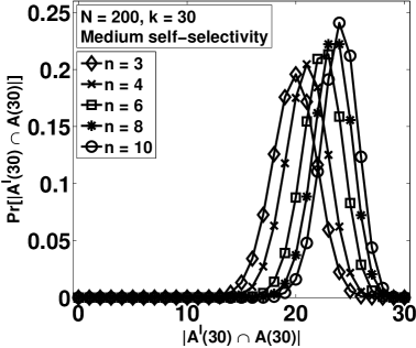
Figure 1: pmf of $|{\cal A}^{I}(30)\!\cap\!{\cal A}(30)|$ when $n\!=\!3,4,6,8,10$ and papers are submitted with medium self-selectivity.

	$n=3$	$n=4$	$n=6$	$n=8$	$n=10$
$E[I_{1}]$	0.9832	0.9931	0.9986	0.9996	0.9999
$E[I_{5}]$	4.6854	4.8284	4.9352	4.9723	4.9869
$E[I_{10}]$	8.7763	9.1643	9.5576	9.7446	9.8426
$E[I_{30}]$	19.8270	20.960	22.400	23.328	23.980
$\mbox{Var}[I_{1}]$	0.0165	0.0067	0.0014	0.0004	0.0001
$\mbox{Var}[I_{5}]$	0.2942	0.1701	0.0654	0.0280	0.0132
$\mbox{Var}[I_{10}]$	1.0793	0.7793	0.4370	0.2586	0.1609
$\mbox{Var}[I_{30}]$	4.1210	3.7710	3.2934	2.9580	2.7121

Table 4: Expectation and variance of $I_{1}$, $I_{5}$, $I_{10}$, and $I_{30}$ when we increase number of reviews per paper, $n\!=\!3,4,6,8,10$, and papers are submitted with medium self-selectivity.

5.2 Effect of Intrinsic Quality

Here, we explore the effect of intrinsic quality (or self-selectivity) of papers on the conference recommendation system. Specifically, we consider four representative types of self-selectivity of papers: high, medium, low and random self-selectivity specified by Eq. (1) $-$ (4) respectively. We explore the effect of self-selectivity of papers on the homogeneous conference recommendation system specified in Section 5.1 with each paper receiving three reviews, or $n\!=\!3$. We use the following notations to present our results:

H-S-S: high self-selectivity specified in Eq. (1).

M-S-S: medium self-selectivity specified in Eq. (2).

L-S-S: low self-selectivity specified in Eq. (3).

R-S-S: random self-selectivity specified in Eq. (4).

The numerical results of the pmf of $|{\cal A}^{I}(30)\cap{\cal A}(30)|$ is shown in Fig. 2. The numerical results of the expectation and variance of $I_{1}$, $I_{5}$, $I_{10}$ and $I_{30}$ are shown in Table 5.

In Fig. 2, the horizontal axis represents the number of top 30 papers that got finally accepted, or $|{\cal A}^{I}(30)\cap{\cal A}(30)|$. The vertical axis shows the corresponding probability. From Fig. 2 we could see that as the self-selectivity type varies in the order of high, low, medium, random self-selectivity, the corresponding mass probability distribution curve moves towards right. In other words, the accuracy of the conference recommendation system corresponding to the random self-selectivity is the highest followed by medium, low and high self-selectivity. From Table 5 we have the following observations. When papers are submitted with medium, low or random self-selectivity, around 20 papers from the top 30 papers will be accepted. It is interesting to note that the chance of accepting the best paper is invariant to these three self-selectivity types, since the corresponding three values of $E[I_{1}]$ are all around 0.98. This statement also holds for top ten papers. But when papers are submitted with high self-selectivity, the accuracy of the conference recommendation system is remarkably lower than that the other three self-selectivity types. Specifically, only a small number, around 13.2, of papers from the top 30 papers will be accepted. Even the best paper will get rejected with high probability, around 0.46. This statement also holds for top ten or top five papers. The variance corresponding to the high self-selectivity is the highest among those four, which reflects that the results of the conference recommendation system is the least accurate and more likely to depart from the expectation. Hence, for a prestigious conference, i.e., SIGCOMM, assume papers are submitted with high self-selectivity, and if the conference insists to have a small technical program committee with reviewers having moderate reviewing workload, say $n\!=\!3$, the final recommendation may not be accurate.

Lessons learned: When reviewers are non-biased fair and critical, the above simple conference review system is quite accurate except when papers are of high self-selectivity. In that case, one may explore other means to improve the accuracy. Again, there are number of interesting questions to explore, i.e., how large the reviewing workload do we need to have an accurate recommendation?

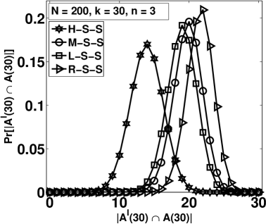
Figure 2: pmf of $|{\cal A}^{I}(30)\!\cap\!{\cal A}(30)|$ when $n\!=\!3$ and papers are submitted with high, medium, low or random self-selectivity.

	H-S-S	M-S-S	L-S-S	R-S-S
$E[I_{1}]$	0.5401	0.9832	0.9788	0.9846
$E[I_{5}]$	2.6250	4.6950	4.6082	4.7599
$E[I_{10}]$	5.0687	8.7736	8.5162	9.0810
$E[I_{30}]$	13.2258	19.8270	18.9798	21.5821
$\mbox{Var}[I_{1}]$	0.2437	0.0165	0.0208	0.0151
$\mbox{Var}[I_{5}]$	1.2236	0.2942	0.3698	0.2314
$\mbox{Var}[I_{10}]$	2.3933	1.0793	1.2491	0.8275
$\mbox{Var}[I_{30}]$	5.4420	4.1210	4.2888	3.5473

Table 5: Expectation and Variance of $I_{1}$, $I_{5}$, $I_{10}$, and $I_{30}$ when $n\!=\!3$ and papers are submitted with high, medium, low or random self-selectivity.

5.3 Effect of Number of Reviews per Paper

Here we consider a homogeneous conference recommendation system specified in Section 5.1. We select one probability measure, expectation of acceptance, to study. The numerical results of $E[I_{1}]$, $E[I_{5}]$, $E[I_{10}]$ and $E[I_{30}]$ are shown in Fig. 3.

In Fig. 3, the horizontal axis represents the number of reviews per paper, or $n$. The vertical axis shows the corresponding expectation. From Fig. 3, we have the following observations. When we increase the number of reviews per paper, or $n$, the expectation increased, which reflects the improvement in accuracy of the conference recommendation system. As the self-selectivity type varies in the order of high, low, medium, random self-selectivity, the expectation curve shifts toward up. In other words, the accuracy corresponding to the random self-selectivity is the highest followed by medium, low, high self-selectivity. It is interesting to note that the best paper is invariant of the workload, except for papers with high self-selectivity. This statement also holds for the top five or ten papers. When papers are highly self-selective, the accuracy of the conference recommendation system is remarkably lower than the other three self-selectivity types. Especially, when the reviewing workload is low, say $n\!=\!3$, with less than 15 papers from the top 30 papers will get accepted. This holds even for the best paper, which only has a probability of less than 0.6 of being accepted when $n\!=\!3$. Same can be said for the top five or top ten papers. In closing, for papers with high self-selectivity, and we may have to increase the reviewing workload to at least $n\!\geq\!7$ such that we have a strong guarantee that the best paper will be accepted.

Lessons learned: If reviewers are non-biased and fair, using the above simple conference review system achieves relatively high accuracy except when papers are of high self-selectivity. In that case, we have to increase the workload to $n\!\geq\!7$ to improve the system. Again, there are number of interesting questions to explore, i.e., is increasing the workload the only way to improve the conference recommendation system? Can we improve it by using different voting rule or tie breaking rule?

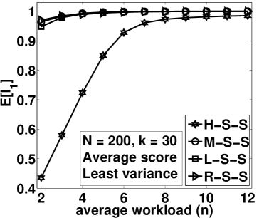
(a) # of top 1 papers get in

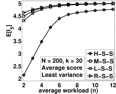
(b) # of top 5 papers get in

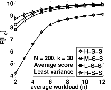
(c) # of top 10 papers get in

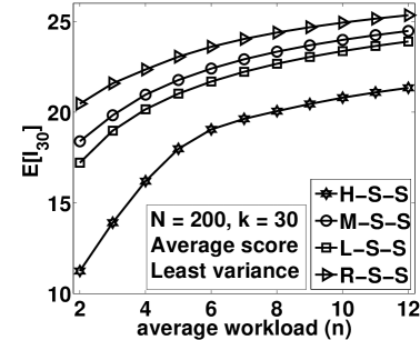
(d) # of top 30 papers get in

Figure 3: Expectation of $I_{1}$, $I_{5}$, $I_{10}$, and $I_{30}$ when we vary number of reviews per paper $n\!=\!2,\ldots,12$, with papers are from high, low, medium or random self-selectivity.

5.4 Effect of Voting Rules

In this section we explore the effect of voting rules on the accuracy of conference recommendation system. Specifically, we will evaluate the performance of the following three representative voting rules:

Average score rule (${\cal V}_{as}$): specified by

$$\gamma_{i}=\sum\nolimits_{S\in\mathcal{S}^{i}}S/|\mathcal{S}^{i}|.$$ (27)

Eliminate the highest & lowest score rule (${\cal V}_{ehl}$): eliminate the highest and lowest score of each paper, and calculate the average score of each paper by the remaining scores, or

$$\gamma_{i}=\left(\sum\nolimits_{S\in\mathcal{S}^{i}}S-\mbox{ max }\{\mathcal{S}^{i}\}-\mbox{ min }\{\mathcal{S}^{i}\}\right)/(|\mathcal{S}^{i}|-2).$$ (28)

Punish low scores rule (${\cal V}_{pl}$): punish the low scores. Specifically, a low score, or 1, brings the an extra punishment of decreasing its score by $\eta$, or

$$\gamma_{i}=\sum\nolimits_{S\in\mathcal{S}^{i}}S/|\mathcal{S}^{i}|-\eta|\{S\>|\>S=1,S\in\mathcal{S}^{i}\}|.$$ (29)

Let us set the punishment $\eta$ to be 0.5 throughout this paper.

We use the least variance rule for tie breaking and we choose expectation as our performance measure. We evaluate the accuracy of these three voting rules on the conference recommendation system specified in Section 5.1. The numerical results of expectation of $I_{30}$ are shown in Fig. 4. The numerical results of expectation of $I_{1}$ and $I_{5}$ for high self-selectivity submissions are shown in Fig. 5. The numerical results of $E[I_{1}]$, $E[I_{5}]$, and $E[I_{10}]$ when $n=3$ are shown in Table 6.

In Fig. 4 and 5 the horizontal axis represents the number of reviews per paper, or $n$. The vertical axis shows corresponding expectation. From Fig. 4, we have the following observations. When we increase $n$, the expectation $E[I_{30}]$ corresponding to each voting rule increased, which reflects that the accuracy of the conference recommendation system increased. From Fig. 4(a), we see that when submitted papers are of high self-selectivity, the expectation curves overlapped together. In other words, for high self-selectivity papers, these three voting rules are similar. From Fig. 4(b) we see that for submitted papers with medium self-selectivity, the average score rule and punish low scores rule have the same degree of accuracy, and the eliminate highest and lowest score rule has slightly higher accuracy than the other two voting rules. This statement also holds for the random self-selectivity submissions as shown in Fig. 4(d). From Fig. 4(c), we see that when submitted papers are of low self-selectivity, all three voting rules have nearly the same accuracy but the punish low scores rule has slightly lower accuracy. From Table 6, we observe that when $n\!=\!3$, the chance of accepting the best paper is invariant of these voting rules, unless when submitted papers are of high selectivity, since $E[I_{1}]$ is around 0.98 for medium, low and random self-selectivity papers. This statement also holds for the top five and the top ten papers. When papers are submitted with high self-selectivity, the chance of accepting the best paper is low, in fact, it is less than 0.6. The same statements holds for the top five and top ten papers. From Fig. 5, we see that when papers submitted with high self-selectivity, the expectation curves overlapped together. And for each voting rule we have to increase the reviewing workload to at least seven such that we have a strong guarantee that the best paper or the top five papers will get accepted.

Lessons learned: These three voting rules have comparable accuracy, no rule can outperform others remarkably. Thus the improvement of conference recommendation system by voting rules is limited. For each voting rule, we till have to increase the average workload to at least seven to have a strong guarantee that the best paper will get in. Again, there are number of interesting questions to explore, i.e., how about the tie-breaking rules?

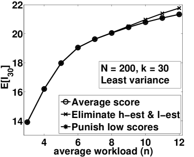
(a) High self-selectivity

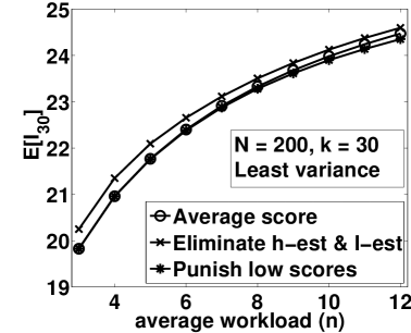
(b) Medium self-selectivity

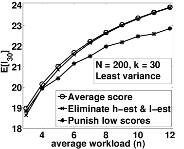
(c) Low self-selectivity

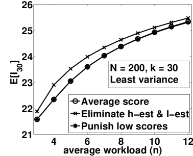
(d) Random self-selectivity

Figure 4: $E[I_{30}]$ for three voting rules: ${\cal V}_{as}$, ${\cal V}_{ehl}$, and ${\cal V}_{pl}$.

	${\cal V}_{as}$	${\cal V}_{ehl}$	${\cal V}_{pl}$
High self-selectivity
$E[I_{1}]$	0.5793	0.5793	0.5793
$E[I_{5}]$	2.8078	2.8078	2.8077
$E[I_{10}]$	5.4028	5.4026	5.4026
Medium self-selectivity
$E[I_{1}]$	0.9832	0.9911	0.9832
$E[I_{5}]$	4.6950	4.7733	4.6950
$E[I_{10}]$	8.7763	8.9641	8.7763
Low self-selectivity
$E[I_{1}]$	0.9788	0.9741	0.9746
$E[I_{5}]$	4.6082	4.5616	4.5691
$E[I_{10}]$	8.5162	8.4032	8.4297
Random self-selectivity
$E[I_{1}]$	0.9846	0.9873	0.9846
$E[I_{5}]$	4.7599	4.7937	4.7599
$E[I_{10}]$	9.0810	9.1791	9.0810

Table 6: Expectation of $E[I_{1}]$, $E[I_{5}]$, and $E[I_{10}]$ for three voting rules: $\mathcal{V}_{as}$, $\mathcal{V}_{ehl}$, and $\mathcal{V}_{pl}$ when $n=3$

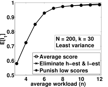
(a) # of top 1 paper get in

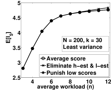
(b) # of top 5 papers get in

Figure 5: Expectation of $E[I_{1}]$, $E[I_{5}]$ for three voting rules: ${\cal V}_{as}$, ${\cal V}_{ehl}$, and ${\cal V}_{pl}$ for high self-selectivity submission.

5.5 Effect of Tie Breaking Rules

In this section we explore the effect of tie breaking rules on conference recommendation system. Specifically, we evaluate the performance of the following four representative tie breaking rules:

Least variance (${\cal T}_{var}$): select one with least variance, if there is still tie, perform random selection.

Largest max score (${\cal T}_{maxs}$): select one with the largest max score, if there is still tie, perform random selection.

Largest min score (${\cal T}_{mins}$): select one with the largest min score, if there is still tie, perform random selection.

Largest medium score (${\cal T}_{meds}$): select one with the largest medium score, if there is still tie, perform random selection.

To evaluate the performance of these four tie breaking rules, let us select a voting rule: average score rule and we use expectation as our performance measure. We evaluate the performance of these four tie breaking rules on the conference recommendation system specified in Section 5.1. The numerical results of $E[I_{30}]$ are shown in Fig. 6. The numerical results of $E[I_{1}]$ and $E[I_{5}]$ for high self-selectivity papers are shown in Fig. 7. The numerical results of $E[I_{1}]$, $E[I_{5}]$, and $E[I_{10}]$ when $n=3$ are shown in Table 7.

In Fig. 6 and 7, the horizontal axis represents the number of reviews per paper, or $n$. The vertical axis shows the corresponding expectation. From Fig. 6, we could have the following observations. When we increase the reviewing workload, the expectation $E[I_{30}]$ corresponding to each tie breaking rule increased, which reflects that the accuracy of the conference recommendation system increased. From Fig. 6(a) and 6(c), we could see that when submitted papers are of high or low self-selectivity, the expectation curves corresponding to these four tie breaking rules overlapped together. In other words, these four rules have the same accuracy. From Fig. 6(b) and 6(d), we see that when submitted papers are of medium or random self-selectivity, the expectation curves corresponding to these four tie breaking rules bunched together and the largest medium score rule has a slightly higher accuracy than others. From Table 7, we see that when $n\!=\!3$, the chance of accepting the best paper is invariant of tie breaking rules, unless when submitted papers are of high self-selectivity, since values of $E[I_{1}]$ corresponding to medium, low or random self-selectivity are all around 0.98. This statement also holds for the top five and top ten papers. When submitted papers are of high self-selectivity, the chance of the best paper being accepted is low, or less than 0.6. The same statements holds for the top five and top ten papers. From Fig. 7, we see that for each tie breaking rule, we still have to increase the reviewing workload $n$ to at least 7 so as to have a strong guarantee that the best paper or the top five papers will get accepted.

Lessons learned: These four tie breaking rules have comparable accuracy, no rule can outperform others remarkably. Thus, the improvement of conference recommendation system by tie breaking rules is limited. For each tie breaking rule, we till have to increase the reviewing workload $n$ to at least seven to have a strong guarantee that the best paper will get in.

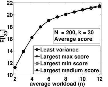
(a) High self-selectivity

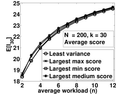
(b) Medium self-selectivity

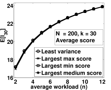
(c) Low self-selectivity

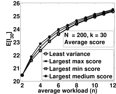
(d) Random self-selectivity

Figure 6: Expectation of $E[I_{30}]$ for four tie breaking rules: ${\cal T}_{var}$, ${\cal T}_{maxs}$, ${\cal T}_{mins}$, and ${\cal T}_{meds}$.

	${\cal T}_{var}$	${\cal T}_{maxs}$	${\cal T}_{mins}$	${\cal T}_{meds}$
High self-selectivity
$E[I_{1}]$	0.5793	0.5793	0.5793	0.5793
$E[I_{5}]$	2.8078	2.8077	2.8077	2.8078
$E[I_{10}]$	5.4026	5.4026	5.4026	5.4026
Medium self-selectivity
$E[I_{1}]$	0.9832	0.9880	0.9832	0.9907
$E[I_{5}]$	4.6951	4.7514	4.6951	4.7755
$E[I_{10}]$	8.7764	8.9311	8.7765	8.9831
Low self-selectivity
$E[I_{1}]$	0.9788	0.9787	0.9788	0.9886
$E[I_{5}]$	4.6083	4.5989	4.6074	4.6040
$E[I_{10}]$	8.5164	8.4723	8.5102	8.3990
Random self-selectivity
$E[I_{1}]$	0.9846	0.9858	0.9846	0.9872
$E[I_{5}]$	4.7599	4.7747	4.7599	4.7926
$E[I_{10}]$	9.0810	9.1239	9.0810	9.1761

Table 7: Expectation of $E[I_{1}]$, $E[I_{5}]$, and $E[I_{10}]$ for four tie breaking rules: ${\cal T}_{var}$, ${\cal T}_{maxs}$, ${\cal T}_{mins}$, and ${\cal T}_{meds}$ when $n\!=\!3$.

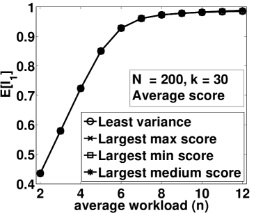
(a) # of top 1 paper get in

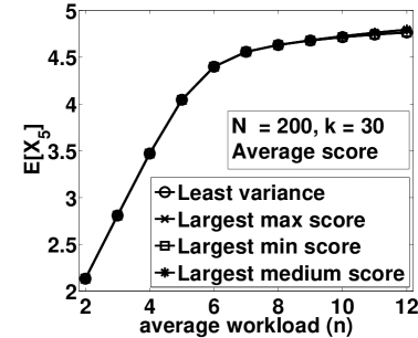
(b) # of top 5 papers get in

Figure 7: Expectation of $E[I_{1}]$, $E[I_{5}]$ for four tie breaking rules: ${\cal T}_{var}$, ${\cal T}_{maxs}$, ${\cal T}_{mins}$, and ${\cal T}_{meds}$ for high self-selectivity submission.

5.6 Effect of Reviewers Type – two types case

We extend the homogeneous conference recommendation system specified in Section 5.1 to a heterogeneous conference recommendation system, for which papers and reviewers can be of different types. Specifically, we consider papers and reviewers are of two types (e.g. system or theory). If paper-reviewer matches in the same type, the critical degree is high, else the critical degree is low. Here we explore the effect of the fraction that paper-reviewer matches in the same type on the accuracy of the recommendation. We use expectation as our performance measure and we set the number of review per paper in this heterogeneous recommendation system be four, or $n\!=\!4$. We vary the fraction of paper-reviewer that matches in the same type from 0.1 to 1. Before showing our results, let us specify $\sigma(c^{i}_{j})$ derived in Eq. (6): if papers-reviewer matches in the same type, $\sigma(c^{i}_{j})\!=\!0.5$, otherwise $\sigma(c^{i}_{j})\!=\!2$. The numerical results of $E[I_{1}]$, $E[I_{5}]$, $E[I_{10}]$, and $E[I_{30}]$ are shown in Fig. 8.

In Fig. 8, the horizontal axis represents the the fraction that paper-reviewer matches in the same type. The vertical axis shows the corresponding expectation. From Fig. 8, we have the following observations. When we increase the matching fraction, the expectation $E[I_{1}]$, $E[I_{5}]$, $E[I_{10}]$, and $E[I_{30}]$ increased. In other words, the accuracy of the conference recommendation system increased when more paper-reviewer matches in the same type. It is interesting to see that the expectation $E[I_{1}]$, $E[I_{5}]$, $E[I_{10}]$ and $E[I_{30}]$ increase in a linear rate and the rate corresponding to the high self-selectivity is the highest, and the random self-selectivity is the lowest. When papers are submitted with medium, low or random self-selectivity, the chance of accepting the best paper is invariant of the matching fraction, since the corresponding values of $E[I_{1}]$ are approximately equal to 1 when the matching fraction is 0 and increased slightly when matching faction increased to 1. This statement also holds for the top five papers. When submitted papers are highly self-selective, the accuracy of the system is very sensitive to the matching fraction, this is because $E[I_{1}]\!\approx\!0.5$, $E[I_{10}]\!\approx\!5$ and $E[I_{30}]\!\approx\!13$ when matching fraction is 0, and $E[I_{1}]\!\approx\!0.9$, $E[I_{10}]\!\approx\!8$ and $E[I_{30}]\!\approx\!20$ when matching fraction is 1.

Lessons learned: If reviewers’ preference and papers match, it can significantly affect the accuracy of the conference recommendation system. This is especially true for submitted papers which are of high self-selectivity (or prestigious conferences). To achieve this, it is especially important to select the appropriate technical program committee members to match the research topics since it can greatly influence the accuracy of the final recommendation.

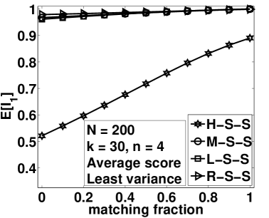
(a) # of top 1 papers get in

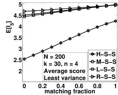
(b) # of top 5 papers get in

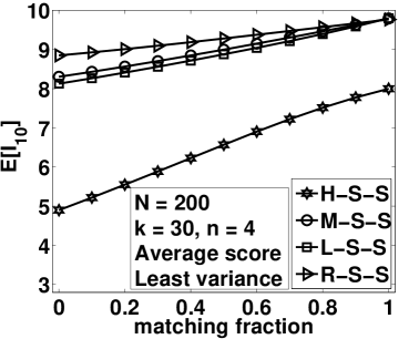
(c) # of top 10 papers get in

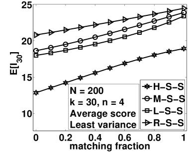
(d) # of top 30 papers get in

Figure 8: Impact of paper-reviewing matching

5.7 Effect of Reviewers type – many types case

We now generalize the types of papers or reviewers of a conference recommendation system specified in Section 5.6 to many types. We explore the effect of reviewer types on the accuracy of different voting rules. Specifically, we consider the following four representative voting rules: Average score (${\cal V}_{as}$), Eliminate the highest & lowest (${\cal V}_{ehl}$) , Punish low scores (${\cal V}_{pl}$) as given by Equation (27) $-$ (29). We also consider the Weighted average (${\cal V}_{wa}$) rule: The average score of paper $P_{i}$ is weighted on $e^{i}_{j}$, where $j\!=\!1,\ldots,n_{i}$, the declared expertise level of reviewer ${\cal R}(S^{i}_{j})$ who selects topics related to $P_{i}$, or

$$\gamma_{i}=\sum\nolimits_{j=1}^{n_{i}}S^{i}_{j}e^{i}_{j}\left[\sum\nolimits_{j=1}^{n_{i}}e^{i}_{j}\right]^{-1}.$$ (30)

We consider the least variance rule for tie breaking and we use expectation as our performance measure. In this evaluation, papers and reviewers are randomly matched. Before showing our results, let us specify two functions that related to model for reviewers types: the first one is $\sigma(c^{i}_{j})$ within the probability distribution for score $S^{i}_{j}$ derived in Eq. (6), which is specified by the following linear function

$$\sigma(c^{i}_{j})=0.5+1.5[1-c^{i}_{j}],$$

the second one is a monotonic increasing function $f(\mu)$ within Eq. (9), which is specified by the following linear function

$$f(\mu)=\mu.$$

We set $l$ to be 3, thus $e^{i}_{j}\in\{1,2,3\}$. The numerical results of $E[I_{30}]$ are shown Fig. 9.

In Fig. 9, the horizontal axis represents the number of reviews per paper, or $n$. The vertical axis shows the corresponding expectation. From Fig. 9, we have the following observations. When submitted papers are of high self-selectivity , the expectation curves corresponding to these four voting rules overlapped together. In other words, these four rules have the same accuracy for high self-selectivity submissions. When submitted papers of low self-selectivity, the punish low scores rule has the lowest accuracy than the other three voting rules which have nearly the same accuracy. When submitted papers of medium self-selectivity, the weighted average scoring rule and the eliminate highest and lowest score rule have nearly the same accuracy, and the weighted average scoring rule has slightly higher accuracy than the average scoring rule and punish low scores rule . This statement also holds for the submitted papers with random self-selectivity.

Lessons learned: When papers and reviewers are of many types and papers and reviewers are randomly matched, weighted average score rule can have slightly higher accuracy than average score rule and punish low scores rule , and it has nearly the same accuracy with eliminate highest and lowest score rule. We have the following similar observations in Section 5.4: these four voting rules have comparable accuracy, no rule can outperform others, thus the improvement of conference recommendation system by voting rules is limited. Again, there are number of interesting questions to explore, i.e., is the accuracy sensitive to anomaly behavior?

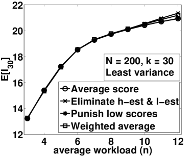
(a) High self-selectivity

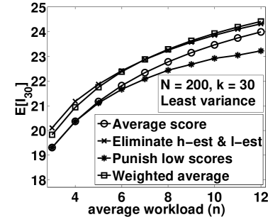
(b) Medium self-selectivity

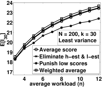
(c) Low self-selectivity

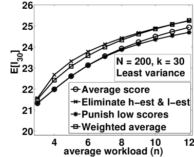
(d) Random self-selectivity

Figure 9: Expectation of $I_{30}$ for four voting rules: ${\cal V}_{as}$, ${\cal V}_{ehl}$, ${\cal V}_{pl}$ and ${\cal V}_{wa}$.

5.8 Effect of Anomaly Behavior – Random Scoring

Let us explore the effect of an anomaly behavior on the accuracy of a conference recommendation system. Specifically, we consider one potential anomaly behavior: random scoring behavior, under which a misbehaving reviewer gives a random score to any paper she reviews regardless of the quality of that paper. We vary the fraction of anomaly behavior from 0.1 to 1 and we use expectation as our performance measure. We explore the effect of anomaly behavior on the conference recommendation system specified in Section 5.1 with number of reviews per paper $n\!=\!4$. The numerical results of $E[I_{1}]$, $E[I_{5}]$, $E[I_{10}]$, and $E[I_{30}]$ are shown in Fig. 10.

In Fig. 10, the horizontal axis represents the fraction of these misbehaving reviewers. The vertical axis shows the corresponding expectation. From Fig. 10, we have the following observations. When we increase the fraction of anomaly reviewers, the expectation decreased. In other words, the more anomaly reviewers, the lower is the accuracy of the conference recommendation system. It is interesting to note that the accuracy of the conference recommendation system decreases in a nearly linear rate. From Fig. 10(a), we see that for low self-selectivity papers, the chance of accepting the best paper can withstand a small fraction of misbehaving reviewers, say around 10%. This statement holds for the top five papers. When submitted papers are of high self-selectivity, around 40% of misbehaving reviewers can drastically disrupt the accuracy of a conference recommendation system. Because for this case, less than ten papers from the top 30 papers will get accepted, and less than four papers from the top ten papers will get accepted. Even the best paper can only be accepted with the probability of less than 0.4. When papers are submitted with medium, low or random self-selectivity, around 60% misbehaving reviewers can drastically disrupt the accuracy of a conference recommendation system.

An interesting question is that which voting rule is more robust against this type of misbehaving reviewers? Here we evaluate three voting rules: average score rule, eliminate highest and lowest and punish low scores given by Equation (27) $-$ (29). We use expectation as our performance measure. The numerical results of $E[I_{30}]$ are shown in Fig. 11.

In Fig. 11, the horizontal axis represents of the fraction of misbehaving reviewers. The vertical axis shows the corresponding expectation. From Fig. 11, we have the following observations. When we increase the fraction of anomaly reviewers, the expectation decreased. From Fig. 11(c), we see that when submitted papers are of low self-selectivity, the expectation curves corresponding to these three voting rules overlapped together. In other words, for the low self-selectivity papers, these three voting rules have the same robustness. From Fig. 11(b), 11(d), we see that when submitted papers are of medium or random self-selectivity, eliminate highest and lowest score rule are slightly more robust than the other two rules. From Fig. 11(a), we observe that when submitted papers of high self-selectivity, these three voting rules have the same robustness when the fraction of anomaly reviewer is less than 30%, and when it is higher than 30%, eliminate highest and lowest voting rule are more robust than the other two rules.

Lessons learned: Random anomaly behavior can significantly affect the accuracy of the conference recommendation system. This is especially true for submitted papers which are of high self-selectivity (or prestigious conferences). The conference recommendation system suffers significantly from this kind of anomaly behavior, say and 20% of misbehaving reviewers will reduce the probability of the best paper to be accepted to around 0.5. These four voting rules have comparable robustness, no rule can outperform others remarkably, thus to defend this kind of anomaly behavior by voting rules may not be effective. Again, there are number of interesting questions to explore, i.e., how to improve the accuracy of the conference recommendation system?

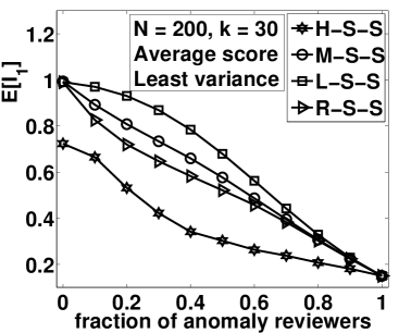
(a) # of top 1 papers get in

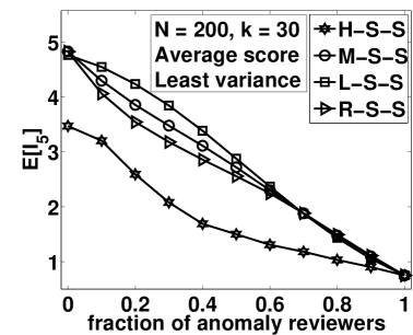
(b) # of top 5 papers get in

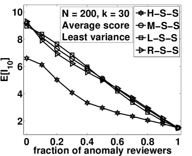
(c) # of top 10 papers get in

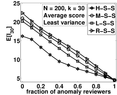
(d) # of top 30 papers get in

Figure 10: Impact of random anomaly behavior when $n\!=\!4$.

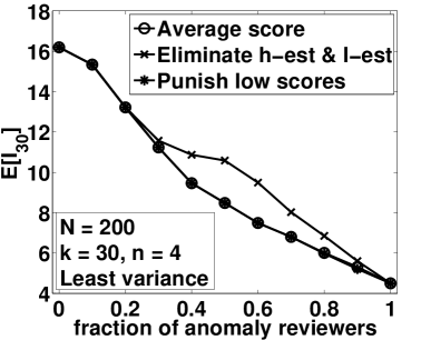
(a) High self-selectivity

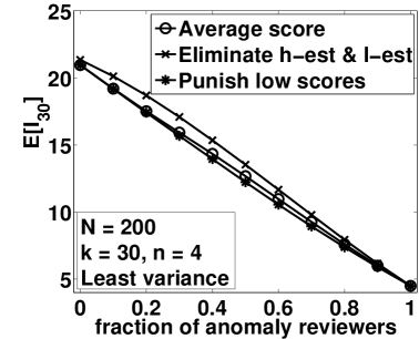
(b) Medium self-selectivity

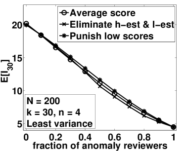
(c) Low self-selectivity

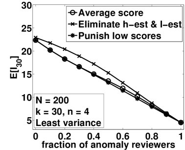
(d) Random self-selectivity

Figure 11: Robustness of three voting rules: ${\cal V}_{as}$, ${\cal V}_{ehl}$, and ${\cal V}_{pl}$ when $n\!=\!4$.

5.9 Effect of Anomaly Behavior – Bias Scoring

Let us explore the effect of another potential anomaly behavior on the accuracy of a conference recommendation system. Specifically, we consider bias scoring behavior, under which a misbehaving reviewer gives a high score $m$ to a paper if the evaluated quality is low, say less than three, otherwise gives a low score 1 to those papers whose evaluated quality is above three. We vary the fraction of anomaly behavior from 0 to 0.3 and we use expectation as our performance measure. We explore the effect of this type of anomaly behavior on the conference recommendation system specified in Section 5.1 with number of reviews per paper $n\!=\!4$. The numerical results of $E[I_{1}]$, $E[I_{5}]$, $E[I_{10}]$, and $E[I_{30}]$ are shown in Fig. 12.

In Fig. 12, the horizontal axis represents the fraction of these misbehaving reviewers. The vertical axis shows the corresponding expectation. From Fig. 12, we have the following observations. When we increase the fraction of anomaly reviewers slightly, the expectation decreased remarkably. From Fig. 12(a), we see that for low self-selectivity papers, the chance of accepting the best paper can withstand a small fraction of misbehaving reviewers, say around 6%, but for the other three self-selectivity types, even a small fraction of misbehaving reviewers may lead to high inaccuracy. For example, when 6% of reviewers are misbehaving, the best paper only has less than 70% chance of being accepted for the highly self-selective paper submissions and it only has less than 80% chance of being accepted for the submitted papers which are of medium or random self-selectivity. Similar deterioration can be said for the top five papers. Around 15% of misbehaving reviewers can drastically disrupt the accuracy of a conference recommendation system, since less than 15 papers from top 30 papers will get accepted.

Lessons learned: Bias scoring anomaly behavior can significantly affect the accuracy of the conference recommendation system. A small fraction of this kind of misbehaving reviewers can decrease the accuracy of the conference recommendation system dramatically. This is especially true for submitted papers which are of high, medium, or random self-selectivity (prestigious, medium, or newly started conferences). The conference recommendation system suffers severely from this kind of anomaly behavior, say 15% of misbehaving reviewers will disrupt the accuracy of the conference recommendation system.

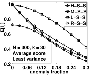
(a) # of top 1 papers get in

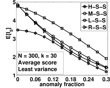
(b) # of top 5 papers get in

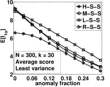
(c) # of top 10 papers get in

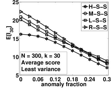
(d) # of top 30 papers get in

Figure 12: Impact of bias scoring anomaly behavior when $n\!=\!4$.

5.10 Improving Conference Recommendation Systems

In reality, most conferences use homogeneous review strategy, with which each paper is reviewed by the same number of reviewers. One obvious advantage of this strategy is its fairness for all papers. But its efficiency in using the workload is low. Here we propose a heterogeneous review strategy that that can increase the efficiency of homogeneous review strategy. In other words, with the same reviewing workload $W$, it has a much higher chance to finally include the top $k$ papers in the final acceptance recommendation. Assume that the the total reviewing workload for the homogeneous review strategy is $W=N*n$. Our heterogeneous review strategy works in two rounds:

Round 1: Eliminate half of the submitted papers using only half of the workload. Specifically, each paper will receive $\lfloor n/2\rfloor$ reviews in the first round. After this reviewing round, apply a voting rule and tie breaking rule to eliminate $N/2$ papers.

Round 2: Select $k$ papers from the remaining $N/2$ papers to accept. Each paper entering this round will receive $2\lceil n/2\rceil$ reviews. After the reviewing process finished, combine their reviews in round 1 and round 2. Then apply a voting rule and a tie breaking rule to select the top $k$ papers to accept.

Definition 3

Let $E[I_{i}\>|\>\mbox{hom}]$ and $E[I_{i}\>|\>\mbox{hetero}]$ represent the expectation of $I_{i}$ under homogeneous or heterogeneous review strategy applied respectively, where $I_{i}$ is defined by Definition 2.

Definition 4

The improvement of heterogeneous review strategy over homogeneous review strategy is:

$$\Delta E[I_{i}]=E[I_{i}\>|\>\mbox{hetero}]-E[I_{i}\>|\>\mbox{hom}],$$

and the improvement ratio is:

$$\Delta E[I_{i}]/E[I_{i}\>|\>\mbox{hom}].$$

We evaluate these two strategies on a conference recommendation system specified in Section 5.1. The numerical results of $\Delta E[I_{30}]$ and $\Delta E[I_{30}]/E[I_{30}\>|\>\mbox{hom}]$ are shown in Fig. 13, where the horizontal axis represents the average reviewing workload $n$. The vertical axis shows the corresponding improvement or improvement ratio. From Fig. 13, we see an improvement of heterogeneous review strategy over homogeneous review strategy. When the reviewing workload is small, say $n\!=\!3$, with heterogeneous review strategy at least one more paper from the top 30 papers will get accepted. For papers with high self-selectivity, we have more improvement wherein three or more papers from the top 30 papers will get accepted. When the average reviewing workload increased to six, the improvement becomes stabilized. When the reviewing workload is three, the improvement is the highest, or around four more papers from the top 30 papers will get accepted for papers submitted with high self-selectivity, and the improvement ratio for this case is around 30%.

An interesting question is that with heterogeneous review strategy, how large the average reviewing workload do we need. We apply our heterogeneous strategy to the conference recommendation system specified in Section 5.3. We use expectation as performance measure. The numerical results of $E[I_{1}]$, $E[I_{5}]$, $E[I_{10}]$ and $E[I_{30}]$ are shown in Fig. 14, where the horizontal axis represents the average reviewing workload $n$. The vertical axis shows the corresponding expectation. From Fig. 14, we see that we need to increase the workload to at least five such that we have a strong guarantee that the best paper will get accepted, which reduces the average review workload by two as compared with the homogeneous review strategy, in which we need to increase the average reviewing workload to at least seven as stated in Section 5.3.

Summary: Lessons learned: Our heterogeneous review strategy uses equal or less resource (e.g., reviewing workload) than the homogeneous review strategy and at the same time, achieve higher accuracy.

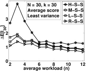
(a) Improvement

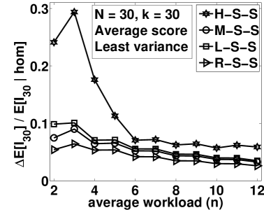
(b) Improvement ratio

Figure 13: Improvement of heterogeneous review strategy on homogeneous review strategy

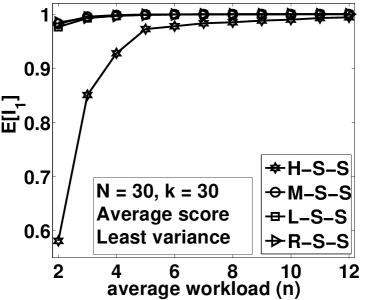
(a) # of top 1 papers get in

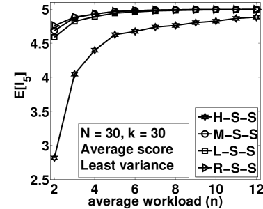
(b) # of top 5 papers get in

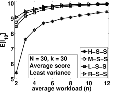
(c) # of top 10 papers get in

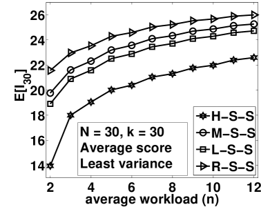
(d) # of top 30 papers get in

Figure 14: Expectation of $I_{1}$, $I_{5}$, $I_{10}$ and $I_{30}$ with heterogeneous review strategy.

6 Related Work

In [8, 9, 14, 21], authors studied peer review systems. Typically, the main issue is the reviewer assignment problem which contains three phrases: specifying the assignment constraint, computing the matching degree between reviewers and submissions, and optimizing the assignment with constraints. Disciplines like information retrieval [8], artificial intelligence [11, 21] and operations research [5, 9, 14], etc address these assignment problems.

Authors in [4, 19, 24, 25] worked on the group recommendation systems and address issues on rating scale and [2, 15, 6] on preference aggregation. Rating is used to show individuals’ preferences, and in [25], authors stated that discrete rating scales (number of rating points) outperform continuous rating scales. In [4], authors evaluated the reliability of rating scales and showed evidence that more rating points will have a more reliable rating. In [19], authors stated that the best rating scale is around five to ten rating points. Preference aggregation is the process to merge the preference of multiple people so as to make recommendations. Basically the aggregation method can be divided into two classes based on the preference type: cardinal ranking or ordinal ranking. For cardinal ranking case, weighted average strategy[16] is the most popular strategy, and it is used in PolyLen. The second class is the ordinal ranking preference, for which, each individual’s preference is shown by a ranked list of a subset of the candidates. For this case, users’ preferences are treated as a set of constraints and a preference aggregation approach attempts to find recommendations that satisfy the constraints of all users[2, 6, 15]. As far as we know, our work is the first that study the mathematical modeling of competitive group recommendation systems and apply it to peer review systems.

7 Conclusions

This is the first paper that provides a mathematical model and analysis on a competitive group recommendation system. We apply it to a conference peer review system and show how various factors may influence the overall accuracy of the final recommendation. We formally analyze the model and through this analysis, we gain the insight on developing a randomized algorithm, which is both computationally efficient and can provide performance guarantees on various performance measures. Number of interesting observations are found, e.g., for a medium tier conference, three reviews per paper are sufficient to achieve high accuracy in the final recommendation, but for some prestigious conferences, we need at least seven reviews per paper. Lastly, we propose a heterogeneous review strategy that requires equal or less reviewing workload but can produce a more accurate recommendation than the homogeneous review strategy. We believe our model and methodology are important building blocks for researchers to study competitive group recommendation systems.

Appendix

Theorem 7

(Chernoff Bound[17]) Let $X_{1},\ldots,X_{n}$ be independent random variables with $X_{i}=1$ with probability $p$ and 0 otherwise. Let $X=\sum_{i=1}^{n}X_{i}$ and let $\mu=E[X]=np$. Then we have

$$\mbox{Pr}[|X-\mu|\geq\epsilon\mu]\leq 2e^{-\mu\epsilon^{2}/3}.$$

In the following lemma we derive a loose bound on the number of simulation rounds $K$ but have a good performance guarantee on the pmd of $I(k)$, or $\mbox{Pr}[I(k)=i],\forall i$ by carefully applying Theorem 7.

Lemma 3

When the following condition holds:

$$K\geq\max\nolimits_{\begin{subarray}{c}i\in\{0,\ldots,k\}\\ \text{Pr}[I(k)=i]\neq 0\end{subarray}}\frac{3\ln(2(k+1)/\delta)}{\mbox{Pr}[I(k)=i]\epsilon^{2}},$$ (31)

then for each $i=0,1,\ldots,k$,

$$\left|\widehat{\mbox{P}}\mbox{r}[I(k)=i]-\mbox{Pr}[I(k)=i]\right|\leq\epsilon\mbox{Pr}[I(k)=i],$$

holds with probability at least $1-\delta/(k+1)$.

Proof: Without lose of any generality, consider the performance guarantee on the approximation of $\mbox{Pr}[I(k)=i]$, where $i=0,1,\ldots,k$. Our goal is to show

$$\left|\widehat{\mbox{P}}\mbox{r}[I(k)=i]-\mbox{Pr}[I(k)=i]\right|\leq\epsilon\mbox{Pr}[I(k)=i].$$

Let $\mathbf{I}_{ij}$ be an indicator random variable defined by

$$\mathbf{I}_{ij}=\left\{\begin{array}[]{ll}1&\mbox{if in $j$-th round, $|\mathcal{A}^{I}(k)\cap\mathcal{A}(k)|=i$}\\ 0&\mbox{otherwise}\end{array},\right.$$

where $j=1,\ldots,K$. There are two cases to explore:
Case 1: $\mbox{Pr}[I(k)=i]=0$. The physical meaning implies that the event $I(k)=i$ never happen, which result in $\mathbf{I}_{ij}=0$ for all $j=0,1,\ldots,K$. Hence, $\widehat{\mbox{P}}\mbox{r}[I(k)=i]=\sum_{j=1}^{K}\mathbf{I}_{ij}/K=0$. Then we have

$$\left|\widehat{\mbox{P}}\mbox{r}[I(k)=i]-\mbox{Pr}[I(k)=i]\right|\leq\epsilon\mbox{Pr}[I(k)=i].$$

Case 2: $\mbox{Pr}[I(k)=i]\neq 0$. Since each round runs independently, thus random variables $\mathbf{I}_{i1},\ldots,\mathbf{I}_{iK}$ are independent random variables with $\mathbf{I}_{ij}=1$ with probability $\mbox{Pr}[I(k)=i]$ and 0 otherwise. Let $\mathbf{I}_{i}=\sum_{j=1}^{K}\mathbf{I}_{ij}$. Then $E[\mathbf{I}_{i}]=K\mbox{Pr}[I(k)=i]$. From Algorithm 1 we could see that $\widehat{\mbox{P}}\mbox{r}[I(k)=i]$, the approximate value of $\mbox{Pr}[I(k)=i]$, is given by $\widehat{\mbox{P}}\mbox{r}[I(k)=i]=\mathbf{I}_{i}/K$. Then by applying Theorem 7 we have,

$$\mbox{Pr}\left[|\widehat{\mbox{P}}\mbox{r}[I(k)=i]-\mbox{Pr}[I(k)=i]|\geq\epsilon\mbox{Pr}[I(k)=i]\right]$$

$$=\mbox{Pr}\left[|\mathbf{I}_{i}-K\mbox{Pr}[I(k)=i]|\geq\epsilon K\mbox{Pr}[I(k)=i]\right]$$

$$\leq 2e^{-K\text{Pr}[I(k)=i]\epsilon^{2}/3},$$

by substituting $K$ with Inequality (31), we have

$$\mbox{Pr}\left[|\widehat{\mbox{P}}\mbox{r}[I(k)=i]-\mbox{Pr}[I(k)=i]|\geq\epsilon\mbox{Pr}[I(k)=i]\right]$$

$$\leq\delta/(k+1).$$

Finally the proof of this lemma can be completed by

$$\mbox{Pr}\left[|\widehat{\mbox{P}}\mbox{r}[I(k)=i]-\mbox{Pr}[I(k)=i]|\leq\epsilon\mbox{Pr}[I(k)=i]\right]$$

$$\geq 1-\mbox{Pr}\left[|\widehat{\mbox{P}}\mbox{r}[I(k)=i]-\mbox{Pr}[I(k)=i]|\geq\epsilon\mbox{Pr}[I(k)=i]\right]$$

$$\geq 1-\delta/(k+1).$$

This lemma is proved.  

Lemma 3 shows the performance guarantee on $\mbox{Pr}[I(k)=i]$ with success probability at least $1-\delta/(k+1)$ for each specific $i=0,1,\ldots,k$. Then, what is the success probability for all $i=0,1,\ldots,k$? The answer of this question is stated in the following lemma.

Lemma 4

When the following condition holds:

$$K\geq\max\nolimits_{\begin{subarray}{c}i\in\{0,\ldots,k\}\\ \text{Pr}[I(k)=i]\neq 0\end{subarray}}\frac{3\ln(2(k+1)/\delta)}{\mbox{Pr}\>[I(k)=i]\epsilon^{2}},$$

then

$$\left|\widehat{\mbox{P}}\mbox{r}[I(k)=i]-\mbox{Pr}[I(k)=i]\right|\leq\epsilon\mbox{Pr}[I(k)=i],$$

holds for all $x=0,1,\ldots,k$, with probability at least $1-\delta$.

Proof: Let $E_{i}$ denote the event that $|\widehat{\mbox{P}}\mbox{r}[I(k)=i]-\mbox{Pr}[I(k)=i]|\leq\epsilon\mbox{Pr}[I(k)=i]$ holds. From Lemma 3 we see that for each $i=0,1,\ldots,k$, the condition

$$|\widehat{\mbox{P}}\mbox{r}[I(k)=i]-\mbox{Pr}[I(k)=i]|\leq\epsilon\mbox{Pr}[I(k)=i]$$

holds with probability at least $1-\delta/(k+1)$, thus

$$\mbox{Pr}[E_{i}]\geq 1-\delta/(k+1).$$

Our goal is to derive the probability that condition

$$|\widehat{\mbox{P}}\mbox{r}[I(k)=i]-\mbox{Pr}[I(k)=i]|\leq\epsilon\mbox{Pr}[I(k)=i]$$

holds for all $i=0,1,\ldots,k$. Specifically, the probability that events $E_{0},E_{1},\ldots,E_{k}$ all happens, or

$$\mbox{Pr}[E_{0},\ldots,E_{k}].$$

Note that the physical meaning of $E_{i}$ is that $\widehat{\mbox{P}}\mbox{r}[I(k)=i]$, the approximate value of $\mbox{Pr}[I(k)=i]$, is close to the true value of $\mbox{Pr}[I(k)=i]$. Thus the physical meaning of $\cap_{i\in{\cal F}}E_{i}$, where ${\cal F}\subseteq\{0,\ldots,k\}$, is that the approximate value of $\mbox{Pr}[I(k)=i]$, is close to the true value of $\mbox{Pr}[I(k)=i]$, for all $i\in{\cal F}$. Thus $\cap_{i\in{\cal F}}E_{i}$ happens implies that $\sum_{i\in{\cal F}}\widehat{\mbox{P}}\mbox{r}[I(k)=i]$, the approximate value of $\sum_{i\in{\cal F}}\mbox{Pr}[I(k)=i]$ is close to the real value of $\sum_{i\in{\cal F}}\mbox{Pr}[I(k)=i]$. Since

$$\sum\nolimits_{i\in\overline{{\cal F}}}\widehat{\mbox{P}}\mbox{r}[I(k)=i]-\sum\nolimits_{i\in\overline{{\cal F}}}\mbox{Pr}[I(k)=i]=\sum\nolimits_{i\in{\cal F}}\widehat{\mbox{P}}\mbox{r}[I(k)=i]-\sum\nolimits_{i\in{\cal F}}\mbox{Pr}[I(k)=i],$$

where $\overline{{\cal F}}=\{0,1,\ldots,k\}\backslash{\cal F}$ is the complement of ${\cal F}$, thus we have that $\sum_{i\in{\cal F}}\widehat{\mbox{P}}\mbox{r}[I(k)=i]$ is close to the real value of $\sum_{i\in{\cal F}}\mbox{Pr}[I(k)=i]$ if and only if $\sum_{i\in\overline{{\cal F}}}\widehat{\mbox{P}}\mbox{r}[I(k)=i]$ is close the real value of $\sum_{i\in\overline{{\cal F}}}\mbox{Pr}[I(k)=i]$. Thus $\cap_{i\in{\cal F}}E_{i}$ implies that $\sum_{i\in\overline{{\cal F}}}\widehat{\mbox{P}}\mbox{r}[I(k)=i]$ is close the real value of $\sum_{i\in\overline{{\cal F}}}\mbox{Pr}[I(k)=i]$.

The event $\cap_{i\in{\cal G}}E_{i}$, where ${\cal G}\subseteq\overline{{\cal F}}$, is more likely to happen given the prior information that $\sum_{i\in\overline{{\cal F}}}\widehat{\mbox{P}}\mbox{r}[I(k)=i]$ is close the real value of $\sum_{i\in\overline{{\cal F}}}\mbox{Pr}[I(k)=i]$ than given noting at all. Since $\cap_{i\in{\cal F}}E_{i}$ implies that $\sum_{i\in\overline{{\cal F}}}\widehat{\mbox{P}}\mbox{r}[I(k)=i]$ is close the real value of $\sum_{i\in\overline{{\cal F}}}\mbox{Pr}[I(k)=i]$, thus $\cap_{i\in{\cal G}}E_{i}$, where ${\cal G}\subseteq\overline{{\cal F}}$, is more likely to happen given prior information that $\cap_{i\in{\cal F}}E_{i}$ happens than given nothing at all. Or mathematically,

$$\mbox{Pr}[\cap_{i\in{\cal G}}E_{i}|\cap_{i\in{\cal F}}E_{i}]\geq\mbox{Pr}[\cap_{i\in{\cal G}}E_{i}],$$

where ${\cal G}\subseteq\overline{{\cal F}}$. Based on this fact, we have

$$\mbox{Pr}[E_{0},\ldots,E_{k}]=\prod\nolimits_{i=0}^{k}\mbox{Pr}[E_{i}|\cap_{j\in{\cal F}_{i}}E_{j}]\geq\prod\nolimits_{i=0}^{k}\mbox{Pr}[E_{i}],$$

where ${\cal F}_{i}=\{0,\ldots,k\}/\{0,\dots,i\}$. By substituting $\mbox{Pr}[E_{i}]$ with $\mbox{Pr}[E_{i}]\geq 1-\delta/(k+1)$ we have

$$\mbox{Pr}[E_{0},\ldots,E_{k}]\geq[1-\delta/(k+1)]^{k+1}\geq 1-\delta,$$

which completes the proof.  

In the following lemma we derive the error bound of expectation, or $|{\widehat{E}}[I(k)]-E[I(k)]|$, under the condition that $|\widehat{\mbox{P}}\mbox{r}[I(k)=i]-\mbox{Pr}[I(k)=i]|\leq\epsilon\mbox{Pr}[I(k)=i]$ holds for all $i=0,1,\ldots,k$.

Lemma 5

When the following condition holds:

$$\left|\widehat{\mbox{P}}\mbox{r}[I(k)=i]-\mbox{Pr}[I(k)=i]\right|\leq\epsilon\mbox{Pr}[I(k)=i],$$

for all $i=0,1,\ldots,k$, then

$$\left|{\widehat{E}}[I(k)]-E[I(k)]\right|\leq\epsilon E[I(k)]$$

holds.

Proof: The proof is quite straightforward,

$$\left|{\widehat{E}}[I(k)]\!-\!E[I(k)]\right| \!=\!\left|\sum\nolimits_{i=0}^{k}i\left(\widehat{\mbox{P}}\mbox{r}[I(k)\!=\!i]\!-\!\mbox{Pr}[I(k)\!=\!i]\right)\right|$$

$$\!\leq\!\sum\nolimits_{i=0}^{k}i\left|\widehat{\mbox{P}}\mbox{r}[I(k)\!=\!i]\!-\!\mbox{Pr}[I(k)\!=\!i]\right|$$

$$\!\leq\!\sum\nolimits_{i=0}^{k}\epsilon i\mbox{Pr}[I(k)=i]=\epsilon E[I(k)],$$

which complets the proof.  

In the following, we let $\Delta E[I(k)]={\widehat{E}}[I(k)]-E[I(k)]$ and $\Delta p_{i}=\widehat{\mbox{P}}\mbox{r}[I(k)=i]-\mbox{Pr}[I(k)=i]$. In the following we first derive the bound of $(\Delta E[I(k)])^{2}$, and then apply the bound of $(\Delta E[I(k)])^{2}$ to derive the bound of variance, or $|\widehat{\mbox{V}}\mbox{ar}[I(k)]-\mbox{Var}[I(k)]|$. The bound of $(\Delta E[I(k)])^{2}$ is stated in the following lemma.

Lemma 6

When the following condition holds:

$$\left|\widehat{\mbox{P}}\mbox{r}[I(k)\!=\!i]\!-\!\mbox{Pr}[I(k)\!=\!i]\right|\!\leq\!\epsilon\mbox{Pr}[I(k)\!=\!i]$$

for all $i=0,1,\ldots,k$, then

$$\left(\Delta E[I(k)]\right)^{2}\leq\epsilon^{2}\mbox{Var}[I(k)]$$ (32)

holds.

Proof: First we have $|\Delta p_{i}|\leq\epsilon\mbox{Pr}[I(k)=i]$. It is straightforward to show $\sum\nolimits_{i=0}^{k}\Delta p_{i}=0$, or

$$\sum\nolimits_{i=0}^{k}\Delta p_{i} =\sum\nolimits_{i=0}^{k}\widehat{\mbox{P}}\mbox{r}[I(k)=i]-\sum\nolimits_{i=0}^{k}\mbox{Pr}[I(k)=i]$$

$$=0.$$

Based on this fact, we could have

$$(\Delta E[I(k)])^{2} =\left(\sum\nolimits_{i=0}^{k}i\Delta p_{i}\right)^{2}$$

$$=\left(\sum\nolimits_{i=0}^{k}i\Delta p_{i}-E[I(k)]\sum\nolimits_{i=0}^{k}\Delta p_{i}\right)^{2}$$

$$\leq\left(\sum\nolimits_{i=0}^{k}|i-E[I(k)]|\>|\Delta p_{i}|\right)^{2}.$$ (33)

Then by substituting $|\Delta p_{i}|$ with $|\Delta p_{i}|\leq\epsilon\mbox{Pr}[I(k)=i]$ we have

$$(\Delta E[I(k)])^{2}\leq\left(\sum\nolimits_{i=0}^{k}|i-E[X]|\epsilon\mbox{Pr}[I(k)=i]\right)^{2}$$

by applying Cauchy’s Inequality we have,

$$(\Delta E[I(k)])^{2} \leq\left(\sum\nolimits_{i=0}^{k}\epsilon^{2}\mbox{Pr}[I(k)=i]\right)\left(\sum\nolimits_{i=0}^{k}(i-E[X])^{2}\mbox{Pr}[I(k)=i]\right)$$

$$=\epsilon^{2}\mbox{Var}[I(k)],$$

which completes the proof.  

In the following lemma we apply Lemma 6 to derive the error bound of variance, or $|\widehat{\mbox{V}}\mbox{ar}[I(k)]-\mbox{Var}[I(k)]|$.

Lemma 7

When the following condition holds:

$$\left|\widehat{\mbox{P}}\mbox{r}[I(k)\!=\!i]\!-\!\mbox{Pr}[I(k)\!=\!i]\right|\!\leq\!\epsilon\mbox{Pr}[I(k)\!=\!i]$$

for all $i=0,1,\ldots,k$, then

$$\left|\widehat{\mbox{V}}\mbox{ar}[I(k)]-\mbox{Var}[I(k)]\right|\leq\epsilon(1+\epsilon)\mbox{Var}[I(k)]$$

holds.

Proof: First we can write $\widehat{\mbox{V}}\mbox{ar}[I(k)]-\mbox{Var}[I(k)]$ in the following form:

$$\widehat{\mbox{V}}\mbox{ar}[I(k)]-\mbox{Var}[I(k)] =\sum\nolimits_{i=0}^{k}i^{2}\Delta p_{i}-2E[I(k)]\Delta E[I(k)]-(\Delta E[I(k)])^{2}$$

$$=\sum\nolimits_{i=0}^{k}(i-E[I(k)])^{2}\Delta p_{i}-(E[I(k)])^{2}\sum\nolimits_{i=0}^{k}\Delta p_{i}-(\Delta E[I(k)])^{2}$$

Since $\sum_{i=0}^{k}\Delta p_{i}=0$, thus we have

$$\left|\widehat{\mbox{V}}\mbox{ar}[I(k)]-\mbox{Var}[I(k)]\right| =\left|\sum\nolimits_{i=0}^{k}(i-E[I(k)])^{2}\Delta p_{i}-(\Delta E[I(k)])^{2}\right|$$

$$\leq\sum\nolimits_{i=0}^{k}(i-E[I(k)])^{2}|\Delta p_{i}|+(\Delta E[I(k)])^{2},$$ (34)

by substituting $\Delta p_{i}$ with $|\Delta p_{i}|\leq\epsilon\mbox{Pr}[I(k)=i]$, and substituting $(\Delta E[I(k)])^{2}$ with Inequality (32) we have

$$|\widehat{\mbox{V}}\mbox{ar}[I(k)]-\mbox{Var}[I(k)]|\leq\epsilon(1+\epsilon)\mbox{Var}[I(k)],$$

which completes the proof.  

In the following lemmas, we show how to tradeoff the number of simulation rounds $K$ with the performance guarantees. The tradeoff between $K$ and the performance guarantee on pmf is stated in the following theorem.

Lemma 8

When the following condition holds:

$$K\geq 3\ln(2(k+1)/\delta)/\epsilon^{2},$$ (35)

then for each $i=0,\ldots,k$,

$$\left|\widehat{\mbox{P}}\mbox{r}[I(k)=i]-\mbox{Pr}[I(k)=i]\right|\leq\epsilon\sqrt{\mbox{Pr}[I(k)=i]},$$

holds with probability at least $1-\delta/(k+1)$.

Proof: Without lose of any generality, consider the performance guarantee on the approximation of $\mbox{Pr}[I(k)=i]$, where $i=0,1,\ldots,k$. Our goal is to show

$$\left|\widehat{\mbox{P}}\mbox{r}[I(k)=i]-\mbox{Pr}[I(k)=i]\right|\leq\epsilon\sqrt{\mbox{Pr}[I(k)=i]}.$$

Following similar method in Lemma 3 and the same notations defined in the proof of Lemma 3, we could have the following:
Case 1: $\mbox{Pr}[I(k)=i]=0$. Then $\widehat{\mbox{P}}\mbox{r}[I(k)=i]=0$. Hence

$$\left|\widehat{\mbox{P}}\mbox{r}[I(k)=i]-\mbox{Pr}[I(k)=i]\right|\leq\epsilon\sqrt{\mbox{Pr}[I(k)=i]}.$$

Case 2: $\mbox{Pr}[I(k)=i]\neq 0$. Following similar method in Lemma 3 we have

$$\mbox{Pr}\left[|\widehat{\mbox{P}}\mbox{r}[I(k)=i]-\mbox{Pr}[I(k)=i]|\leq\epsilon\sqrt{\mbox{Pr}[I(k)=i]}\right]$$

$$\geq 1-\mbox{Pr}\left[|\widehat{\mbox{P}}\mbox{r}[I(k)=i]-\mbox{Pr}[I(k)=i]|\geq\epsilon\sqrt{\mbox{Pr}[I(k)=i]}\right]$$

$$=1-\mbox{Pr}\left[|\mathbf{I}_{i}-K\mbox{Pr}[I(k)=i]|\geq\frac{\epsilon K\mbox{Pr}[I(k)=i]}{\sqrt{\mbox{Pr}[I(k)=i]}}\right]$$

$$\geq 1-2e^{-K\epsilon^{2}/3},$$

by substituting $K$ with Inequality (35) we can prove this lemma.  

Using the same method in Lemma 3, we can prove the following lemma.

Lemma 9

When $K\geq 3\ln(2(k+1)/\delta)/\epsilon^{2}$ , then

$$\left|\widehat{\mbox{P}}\mbox{r}[I(k)=i]-\mbox{Pr}[I(k)=i]\right|\leq\epsilon\sqrt{\mbox{Pr}[I(k)=i]}$$

holds for all $i=0,1,\ldots,k$ with probability at least $1-\delta$.

In the following lemma we derive the error bound of expectation, or $|{\widehat{E}}[I(k)]-E[I(k)]|$, under the condition that $|\widehat{\mbox{P}}\mbox{r}[I(k)=i]-\mbox{Pr}[I(k)=i]|\leq\epsilon\sqrt{\mbox{Pr}[I(k)=i]}$ holds for all $i=0,1,\ldots,k$.

Lemma 10

When the following condition holds:

$$\left|\widehat{\mbox{P}}\mbox{r}[I(k)=i]-\mbox{Pr}[I(k)=i]\right|\leq\epsilon\sqrt{\mbox{Pr}[I(k)=i]}$$

holds for all $i=0,1,\ldots,k$, then

$$\left|{\widehat{E}}[I(k)]-E[I(k)]\right|\leq\epsilon\sqrt{(k+1)kE[I(k)]/2}$$

holds.

Proof: First we have $\Delta p_{i}\leq\epsilon\sqrt{\mbox{Pr}[I(k)=i]}$. Then we have the following

$$\left|{\widehat{E}}[I(k)]-E[I(k)]\right| \leq\sum\nolimits_{i=0}^{k}i|\Delta p_{i}|$$

$$\leq\sum\nolimits_{i=0}^{k}\epsilon i\sqrt{\mbox{Pr}[I(k)=i]},$$

by applying Cauchy’s Inequality we have,

$$\left|{\widehat{E}}[I(k)]-E[I(k)]\right| \leq\epsilon\sqrt{\!\!\left(\sum\nolimits_{i=0}^{k}i\right)\!\!\left(\sum\nolimits_{i=0}^{k}i\mbox{Pr}[I(k)=i]\right)}$$

$$=\epsilon\sqrt{(k+1)kE[I(k)]/2},$$

which completes the proof.  

In the following lemma we derive the bound of $(\Delta E[I(k)])^{2}$ under the condition that $|\widehat{\mbox{P}}\mbox{r}[I(k)=i]-\mbox{Pr}[I(k)=i]|\leq\epsilon\sqrt{\mbox{Pr}[I(k)=i]}$ holds for all $i=0,1,\ldots,k$.

Lemma 11

When the following condition holds:

$$\left|\widehat{\mbox{P}}\mbox{r}[I(k)=i]-\mbox{Pr}[I(k)=i]\right|\leq\epsilon\sqrt{\mbox{Pr}[I(k)=i]}$$

holds for all $i=0,1,\ldots,k$, then

$$(\Delta E[I(k)])^{2}\leq\epsilon^{2}(k+1)\mbox{Var}[I(k)]$$ (36)

holds.

Proof: First we have $\Delta p_{i}\leq\epsilon\sqrt{\mbox{Pr}[I(k)=i]}$. From Inequality (Appendix) we have

$$(\Delta E[I(k)])^{2}\leq\left(\sum\nolimits_{i=0}^{k}|i-E[I(k)]|\>|\Delta p_{i}|\right)^{2},$$

by substituting $|\Delta p_{i}|$ with $\Delta p_{i}\leq\epsilon\sqrt{\mbox{Pr}[I(k)=i]}$ we have

$$(\Delta E[I(k)])^{2}\leq\left(\sum\nolimits_{i=0}^{k}|i-E[I(k)]|\>\epsilon\sqrt{\mbox{Pr}[I(k)=i]}\right)^{2},$$

by applying Cauchy’s Inequality we have,

$$(\Delta E[I(k)])^{2} \leq\left(\sum\nolimits_{i=0}^{k}\epsilon^{2}\right)\left(\sum\nolimits_{i=0}^{k}(i-E[I(k)])^{2}\mbox{Pr}[I(k)=i]\right)$$

$$=\epsilon^{2}(k+1)\mbox{Var}[I(k)],$$

which completes the proof.  

In the following lemma we apply Lemma 11 to derive the error bound of variance, or $|\widehat{\mbox{V}}\mbox{ar}[I(k)]-\mbox{Var}[I(k)]|$, under the condition that $|\widehat{\mbox{P}}\mbox{r}[I(k)=i]-\mbox{Pr}[I(k)=i]|\leq\epsilon\sqrt{\mbox{Pr}[I(k)=i]}$ holds for all $i=0,1,\ldots,k$.

Lemma 12

When the following condition holds:

$$\left|\widehat{\mbox{P}}\mbox{r}[I(k)=i]-\mbox{Pr}[I(k)=i]\right|\leq\epsilon\sqrt{\mbox{Pr}[I(k)=i]}$$

holds for all $i=0,1,\ldots,k$, then

$$\left|\widehat{\mbox{V}}\mbox{ar}[I(k)]-\mbox{Var}[I(k)]\right| \leq\epsilon(k+1)\left(\sqrt{(2k+1)\mbox{Var}\>[I(k)]/6}+\epsilon\mbox{Var}\>[I(k)]\right)$$

holds.

Proof: First we have $\Delta p_{i}\leq\epsilon\sqrt{\mbox{Pr}[I(k)=i]}$. From Inequality (Appendix) we have

$$\left|\widehat{\mbox{V}}\mbox{ar}[I(k)]-\mbox{Var}[I(k)]\right| \leq\sum\nolimits_{i=0}^{k}(i-E[I(k)])^{2}|\Delta p_{i}|\!+(\Delta E[I(k)])^{2},$$

by substituting $\Delta p_{i}$ with $|\Delta p_{i}|\leq\epsilon\sqrt{\mbox{Pr}[I(k)=i]}$ we have

$$|\widehat{\mbox{V}}\mbox{ar}[I(k)]-\mbox{Var}[I(k)]| \leq\sum\nolimits_{i=0}^{k}(i-E[I(k)])^{2}\epsilon\sqrt{\mbox{Pr}[I(k)=i]}+(\Delta E[I(k)])^{2},$$

by applying Cauchy’s Inequality we have,

$$|\widehat{\mbox{V}}\mbox{ar}[I(k)]-\mbox{Var}[I(k)]| \leq\epsilon\left(\sum\nolimits_{i=0}^{k}(i-E[I(k)])^{2}\mbox{Pr}[I(k)=i]\right)^{1/2}\left(\sum\nolimits_{i=0}^{k}(i-E[I(k)])^{2}\right)^{1/2}+(\Delta E[I(k)])^{2}$$

$$\leq\epsilon\left((k+1)\sqrt{(2k+1)\!\mbox{Var}[I(k)]/6}\right)+(\Delta E[I(k)])^{2},$$

the proof can be completed by substituting $(\Delta E[X])^{2}$ with Inequality (36).

References

- [1] S. Amer-Yahia, S. Roy, A. Chawlat, G. Das, and C. Yu. Group recommendation: Semantics and efficiency. Proc. of VLDB, 2009.
- [2] J. Baskin and S. Krishnamurthi. Preference aggregation in group recommender systems for committee decision-making. In Proc. of ACM RecSys, 2009.
- [3] L. Boratto and S. Carta. State-of-the-art in group recommendation and new approaches for automatic identification of groups. Information Retrieval and Mining in Distributed Environments, pages 1–20, 2011.
- [4] G. Churchill Jr and J. Peter. Research design effects on the reliability of rating scales: a meta-analysis. Journal of Marketing Research, pages 360–375, 1984.
- [5] W. Cook, B. Golany, M. Kress, M. Penn, and T. Raviv. Optimal allocation of proposals to reviewers to facilitate effective ranking. Management Science, pages 655–661, 2005.
- [6] W. Cook, B. Golany, M. Penn, and T. Raviv. Creating a consensus ranking of proposals from reviewers partial ordinal rankings. Computers & operations research, 34(4):954–965, 2007.
- [7] M. Deshpande and G. Karypis. Item-based top-n recommendation algorithms. ACM TOIS, 22(1):143–177, 2004.
- [8] S. Dumais and J. Nielsen. Automating the assignment of submitted manuscripts to reviewers. In Proc. of ACM SIGIR, 1992.
- [9] D. Hartvigsen, J. Wei, and R. Czuchlewski. The conference paper-reviewer assignment problem. Decision Sciences, 30(3):865–876, 1999.
- [10] J. Herlocker, J. Konstan, L. Terveen, and J. Riedl. Evaluating collaborative filtering recommender systems. ACM TOIS, 22(1):5–53, 2004.
- [11] S. Hettich and M. Pazzani. Mining for proposal reviewers: lessons learned at the national science foundation. In Proc. of SIGKDD’06.
- [12] A. Jameson. More than the sum of its members: challenges for group recommender systems. In Proc. of ACM working conference on Advanced visual interfaces, 2004.
- [13] A. Jameson, S. Baldes, and T. Kleinbauer. Two methods for enhancing mutual awareness in a group recommender system. In Proceedings of ACM working conference on Advanced visual interfaces, 2004.
- [14] M. Karimzadehgan and C. Zhai. Constrained multi-aspect expertise matching for committee review assignment. In Proc. of CIKM’09.
- [15] F. Lorenzi, F. dos Santos, P. Ferreira, and A. Bazzan. Optimizing preferences within groups: a case study on travel recommendation. Advances in Artificial Intelligence-SBIA, pages 103–112, 2008.
- [16] J. Masthoff. Group modeling: Selecting a sequence of television items to suit a group of viewers. User Modeling and User-Adapted Interaction, 14(1):37–85, 2004.
- [17] M. Mitzenmacher and E. Upfal. Probability and computing: Randomized algorithms and probabilistic analysis. Cambridge Univ Pr, 2005.
- [18] M. O connor, D. Cosley, J. Konstan, and J. Riedl. Polylens: A recommender system for groups of users. In Proc. of ECSCW 2001.
- [19] C. Preston and A. Colman. Optimal number of response categories in rating scales: reliability, validity, discriminating power, and respondent preferences. Acta psychologica, 104(1):1–15, 2000.
- [20] P. Resnick and H. Varian. Recommender systems. Communications of the ACM, 40(3):56–58, 1997.
- [21] M. Rodriguez and J. Bollen. An algorithm to determine peer-reviewers. In Proc. of ACM CIKM, 2008.
- [22] B. Sarwar, G. Karypis, J. Konstan, and J. Reidl. Item-based collaborative filtering recommendation algorithms. In Proc. of WWW’01.
- [23] J. Schafer, J. Konstan, and J. Riedi. Recommender systems in e-commerce. In Proc. of ACM EC, 1999.
- [24] E. I. Sparling and S. Sen. Rating: how difficult is it? In Proc. of ACM RecSys, 2011.
- [25] E. Svensson. Comparison of the quality of assessments using continuous and discrete ordinal rating scales. Biometrical Journal, 42(4):417–434, 2000.