Estimation of causal orders in a linear non-Gaussian acyclic model:
a method robust against latent confounders

Abstract

We consider to learn a causal ordering of variables in a linear non-Gaussian acyclic model called LiNGAM. Several existing methods have been shown to consistently estimate a causal ordering assuming that all the model assumptions are correct. But, the estimation results could be distorted if some assumptions actually are violated. In this paper, we propose a new algorithm for learning causal orders that is robust against one typical violation of the model assumptions: latent confounders. We demonstrate the effectiveness of our method using artificial data.

1 Introduction

Bayesian networks have been widely used to analyze causal relations of variables in many empirical sciences [11]. A common assumption is linear-Gaussianity. But this poses serious identifiability problems so that many important models are indistinguishable with no prior knowledge on the structures. Recently, it was shown [9] that use of non-Gaussianity allows the full structure of a linear acyclic model to be identified without pre-specifying any causal orders of variables. The new model, a Linear Non-Gaussian Acyclic Model called LiNGAM [9], is closely related to independent component analysis (ICA) [7].

Existing estimation methods [9, 10] for LiNGAM learn causal orders assuming that all the model assumptions hold. Therefore, these algorithms could return completely wrong estimation results when some of the model assumptions is violated. Thus, in this paper, we propose a new algorithm for learning causal orders that is robust against one typical model violation, i.e., latent confounders. A latent confounder means a variable which is not observed but which exerts a causal influence on some of the observed variables.

The paper is organized as follows. We first review LiNGAM [9] and its extension to latent confounder cases [6] in Section 2. In Section 3, we propose a new algorithm to learn causal orders in LiNGAM with latent confounders. Simulations are conducted in Section 4. We conclude this paper in Section 5.

2 Background: LiNGAM with latent confounders

We briefly review a linear non-Gaussian acyclic model called LiNGAM [9] and an extension of the LiNGAM to cases with latent confounding variables [6].

In LiNGAM [9], causal relations of observed variables $x_{i}$ are modeled as:

$$x_{i} = \sum_{k(j)<k(i)}b_{ij}x_{j}+e_{i},$$ (1)

where $k(i)$ is such a causal ordering of variables $x_{i}$ that they graphically form a directed acyclic graph (DAG) so that no later variable determines, i.e., has a directed path on any earlier variable, $e_{i}$ are external influences, and $b_{ij}$ are connection strengths. In matrix form, the model (1) is written as

$${\bf x} = {\bf B}{\bf x}+{\bf e},$$ (2)

where the connection strength matrix ${\bf B}$ collects $b_{ij}$ and the vectors ${\bf x}$ and ${\bf e}$ collect $x_{i}$ and $e_{i}$. Note that the matrix ${\bf B}$ can be permuted to be lower triangular with all zeros on the diagonal if simultaneous equal row and column permutations are made according to a causal ordering $k(i)$ due to the acyclicity. The zero/non-zero pattern of $b_{ij}$ corresponds to the absence/existence pattern of directed edges. External influences $e_{i}$ follow non-Gaussian continuous distributions with zero mean and non-zero variance and are mutually independent. The non-Gaussianity assumption on $e_{i}$ enables identification of a causal ordering $k(i)$ based on data ${\bf x}$ only [9]. This feature is a big advantage over conventional Bayesian networks based on the Gaussianity assumption on $e_{i}$[11].

Next, LiNGAM with latent confounders [6] can be formulated as follows:

$${\bf x} = {\bf B}{\bf x}+{\bf\Lambda}{\bf f}+{\bf e},$$ (3)

where the difference with LiNGAM (2) is the existence of latent confounding variable vector ${\bf f}$. A latent confounding variable is such an latent variable that is a parent of more than or equal to two observed variables. The vector ${\bf f}$ collects non-Gaussian latent confounders $f_{j}$ with zero mean and non-zero variance $(j=1,\cdots,q)$. Without loss of generality [6], latent confounders $f_{j}$ are assumed to be mutually independent. The matrix ${\bf\Lambda}$ collects $\lambda_{ij}$ which denotes the connection strength from $f_{j}$ to $x_{i}$. For each $j$, at least two $\lambda_{ij}$ are non-zero since a latent confounder is defined to have at least two children. Further, it is assumed [6] that correlation and conditional correlation of $x_{i}$, $f_{i}$ and $e_{i}$ are entailed by the graph structure only, i.e., the zero/non-zero status of $b_{ij}$ and $\lambda_{ij}$. This is a well-known assumption called faithfulness in causal discovery [11].

The central problem of causal discovery based on the latent variable LiNGAM in Equation (3) is to estimate as many of causal orders $k(i)$ and connection strengths $b_{ij}$ as possible based on data ${\bf x}$ only. This is because in many cases only an equivalence class of the true model whose members produce the exact same observed distribution is identifiable[6].

In [6], an estimation method based on overcomplete ICA was proposed. However, overcomplete ICA methods are often not very reliable and get stuck in local optima. Thus, in [2], a method that does not use overcomplete ICA was proposed to first find variable pairs that are not affected by latent confounders and then estimate a causal ordering of one to the other instead of a causal ordering of more than two variables.

3 A hybrid estimation approach

In this section, we propose a new approach for estimating causal orders of more than two variables without explicitly modeling latent confounders. We first provide principles to identify such an exogenous (root) variable and a sink variable that are not affected by latent confounders in the latent variable LiNGAM in Equation (3) (if such variables exist) and next present an estimation algorithm. Recent estimation methods [10, 8] for LiNGAM in Equation (2) and its nonlinear extension [5] learn a causal ordering by finding causal orders one by one either from the top downward or from the bottom upward assuming no latent confounders. We extend these ideas to latent confounder cases.

We first generalize Lemma 1 of [10] for the case of latent confounders.

Lemma 1

Assume that all the model assumptions of the latent variable LiNGAM (3) are met and the sample size is infinite. Denote by $r_{i}^{(j)}$ the residuals when $x_{i}$ are regressed on $x_{j}$: $r_{i}^{(j)}=x_{i}-\frac{{\rm cov}(x_{i},x_{j})}{{\rm var}(x_{j})}x_{j}$ $(i\neq j)$. Then a variable $x_{j}$ is an exogenous variable in the sense that it has no parent observed variable nor latent confounder if and only if $x_{j}$ is independent of its residuals $r_{i}^{(j)}$ for all $i\neq j$. ∎

Next, we generalize the idea of [8] for the case of latent confounders.

Lemma 2

Assume that all the model assumptions of the latent variable LiNGAM (3) are met and the sample size is infinite. Denote by ${\bf x}_{(-j)}$ a vector that contains all the variables other than $x_{j}$. Denote by $r_{j}^{(-j)}$ the residual when $x_{j}$ is regressed on ${\bf x}_{(-j)}$, i.e., $r_{j}^{(-j)}=x_{j}-\mbox{\boldmath$\sigma$}^{T}_{(-j)j}\Sigma_{(-j)}^{-1}{\bf x}_{(-j)},$ where $\Sigma=\left[\begin{array}[]{cc}\sigma_{j}&\mbox{\boldmath$\sigma$}_{j(-j)}^{T}\\ \mbox{\boldmath$\sigma$}_{j(-j)}&\Sigma_{(-j)}\end{array}\right]$ is the covariance matrix of $[x_{j},{\bf x}_{(-j)}^{T}]^{T}$. Then a variable $x_{j}$ is a sink variable in the sense that it has no child observed variable nor latent confounder if and only if ${\bf x}_{(-j)}$ is independent of its residual $r_{j}^{(-j)}$. ∎

The proofs of these lemmas are given in the appendix.

Thus, we can take a hybrid estimation approach that uses these two principles. We first identify an exogenous variable by finding a variable that is most independent of its residuals and remove the effect of the exogenous variable from the other variables by regressing it out. We repeat this until independence of every variable and any of its residuals is statistically rejected. Dependency between every variable and any of its residuals implies that such an exogenous variable in Lemma 1 does not exist or some model assumption of latent variable LiNGAM (3) is violated. Similarly, we next identify a sink variable in the remaining variables by finding a variable that its regressors and its residual are most independent and disregard the sink variable. We repeat this until independence is statistically rejected for every variable. We test pairwise independence between variables and the residuals using a kernel-based independence measure called HSIC [4] and combine the resulting $p$-values using a well-known Fisher’s method [3]. We use Bonferroni correction for multiple comparison dividing the significance level by the maximum number of tests $p$$-$$1$.

Thus, the estimation consists of the following steps:

1. Given a $p$-dimensional random vector ${\bf x}$, a set of its variable subscripts $U$, a $p\times n$ data matrix of the random vector as ${\bf X}$ and a significance level $\alpha$, initialize an ordered list of variables $K_{head}:=\emptyset$ and $K_{tail}:=\emptyset$ and $m:=1$. $K_{head}$ and $K_{tail}$ denote first $|K_{head}|$ orders of variables and last $|K_{tail}|$ orders of variables respectively, where each of $|K_{head}|$ and $|K_{tail}|$ denotes the number of elements in the list.

2. Let $\tilde{{\bf x}}$$=$${\bf x}$ and $\tilde{{\bf X}}$$=$${\bf X}$ and find causal orders one by one from the top downward:

   1. Do the following steps for all $j\in U\setminus K_{head}$: Perform least squares regressions of $\tilde{x}_{i}$ on $\tilde{x}_{j}$ for all $i\in U\setminus K_{head}$ $(i\neq j)$ and compute the residual vectors $\tilde{{\bf r}}^{(j)}$. Then, find a variable $\tilde{x}_{m}$ that is most independent of its residuals:

      $$\tilde{x}_{m}=\arg\max_{j\in U\setminus K_{head}}P_{Fisher}(\tilde{x}_{j},\tilde{{\bf r}}^{(j)}),$$ (4)

      where $P_{Fisher}(\tilde{x}_{j},\tilde{{\bf r}}^{(j)})$ is the $p$-value of the test statistic defined as $-2\sum_{i}\log\{P_{H}(\tilde{x}_{j},\tilde{r}_{i}^{(j)})\}$, where $P_{H}(\tilde{x}_{j},\tilde{r}_{i}^{(j)})$ is the $p$-value of the HSIC.

   2. Go to Step 1 if $P_{Fisher}(\tilde{x}_{m},\tilde{{\bf r}}^{(m)})<\alpha/(p-1)$.

   3. Append $m$ to the end of $K_{head}$ and let $\tilde{{\bf x}}:=\tilde{{\bf r}}^{(m)}$ and $\tilde{{\bf X}}:=\tilde{{\bf R}}^{(m)}$. If $|K_{head}|=p-1$, append the remaining variable subscript to the end of $K_{head}$ and go to Step 4. Otherwise, go back to Step (2a).

3. If $|K_{head}|<p-2$, let ${\bf x}^{\prime}={\bf x}$ and ${\bf X}^{\prime}={\bf X}$ and $U^{\prime}:=U\setminus K_{head}$ and find causal orders one by one from the bottom upward:

   1. Do the following steps for all $j\in U^{\prime}\setminus K_{tail}$: Collect all the variables except $x^{\prime}_{j}$ in a vector ${\bf x}^{\prime}_{(-j)}$. Perform least squares regressions of $x^{\prime}_{j}$ on ${\bf x}^{\prime}_{(-j)}$ and compute the residual ${r^{\prime}}_{j}^{(-j)}$. Then, find such a variable $x^{\prime}_{m}$ that its regressors and its residual are most independent:

      $$x^{\prime}_{m}=\arg\max_{j\in U^{\prime}\setminus K_{tail}}P_{Fisher}({\bf x}^{\prime}_{(-j)},{r^{\prime}}_{j}^{(-j)}).$$ (5)

   2. Go to Step 4 if $P_{Fisher}({\bf x}^{\prime}_{(-m)},{r^{\prime}}_{m}^{(-m)})<\alpha/(p-1)$.

   3. Append $m$ to the top of $K_{tail}$ and let ${\bf x}^{\prime}={\bf x}^{\prime}_{(-m)}$，${\bf X}^{\prime}={\bf X}^{\prime}_{(-m)}$. Go to Step 4 if $|U^{\prime}\setminus K_{tail}|<3$. Otherwise go back to Step (3a).

4. Estimate connection strengths $b_{ij}$ for variables in $K_{head}$ and $K_{tail}$ by doing multiple regression of every variable $x_{i}$ in $K_{head}$ and $K_{tail}$ on all of its non-descendants $x_{j}$ with $k(j)<k(i)$.

Note that our algorithm would output no causal orders in cases that such exogenous variables and sink variables as in Lemmas 1 and 2 do not exist, although the outputs are still correct. One way to learn more causal orders in those cases would be to develop a divide-and-conquer algorithm that divides variables into subsets where such exogenous or sink variables exist and integrates the estimation results on the subsets. This is an important direction of future research.

4 Experiments on artificial data

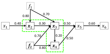
Figure 1: True network used in the simulation. The variables $f_{1}$ and $f_{2}$ were latent confounders. The green contours include variables that share $f_{1}$ or $f_{2}$. The external influences $e_{i}$ are omitted to be shown.

We compared our method with an estimation method for LiNGAM (2) called DirectLiNGAM [10] that does not allow latent confounders and an estimation method for latent variable LiNGAM (3) called Pairwise LvLiNGAM [2]. If there is no latent confounders, all the methods should estimate correct causal orders for enough large sample sizes. The number of variables was 6, and the sample sizes tested were 500, 1000, 2000. The original network used was shown in Figure 1. The $e_{1}$, $e_{4}$ and $f_{1}$ followed a multimodal asymmetric mixture of two Gaussians, $e_{2},e_{5},f_{2}$ followed a double exponential distribution, and $e_{3}$ and $e_{6}$ followed a multimodal symmetric mixture of two Gaussians. The standard deviations of the $e_{i}$ were set so that their signal-to-noise ratios, i.e., ${\rm var}(x_{i})/{\rm var}(e_{i})$$-$$1$ were all ones. The number of trials was 100. The significance level $\alpha$ was 0.05.

First, to evaluate performance of estimating causal orders $k(i)$, we computed the percentage of correctly estimated causal orders in estimated causal orders between two variables (Precision) and the percentage of correctly estimated causal orders in actual causal orders between two variables that share no latent confounders in the true data generating network (Recall). The reason why only pairwise causal orders were evaluated was that Pairwise LvLiNGAM only estimates causal orders of two variables unlike our method and DirectLiNGAM. Tables 2 and 2 show the results. Regarding precisions, our method was comparable to Pairwise LvLiNGAM and the two methods were much better than DirectLiNGAM for all the conditions. Regarding recalls, our method was better than both DirectLiNGAM and Pairwise LvLiNGAM for all the conditions.

Next, to evaluate the performance in estimating connection strengths $b_{ij}$, we computed the root mean square errors between true connection strengths and estimated ones. The root mean square errors for our method and DirectLiNGAM were 0.079 and 0.090 for 500 data points, 0.070 and 0.079 for 1000 data points and 0.015 and 0.057 for 2000 data points, respectively, where our method was more accurate. Note that Pairwise LvLiNGAM does not estimate $b_{ij}$.

Table 1: Precisions

	Sample size
	500	1000	2000
Our method	0.78	0.80	0.80
DirectLiNGAM	0.65	0.64	0.64
Pairwise LvLiNGAM	0.79	0.81	0.81

Table 2: Recalls

	Sample size
	500	1000	2000
Our method	0.97	0.99	0.99
DirectLiNGAM	0.81	0.80	0.81
Pairwise LvLiNGAM	0.86	0.89	0.90

5 Conclusions

We proposed a new algorithm for learning causal orders, which is robust against latent confounders. In experiments on artificial data, our approach learned more causal orders accurately than two existing methods. In future work, we would like to test our method on real-world data including functional magnetic resonance imaging data to analyze causal interactions between brain regions.

Acknowledgments.

S.S and T.W. were supported by KAKENHI #24700275 and #22300054. We thank Patrik Hoyer and Doris Entner for helpful comments.

Appendix: Proofs of the lemmas

Theorem 1 (Darmois-Skitovitch theorem (D-S theorem) [1])

Define two random variables $y_{1}$ and $y_{2}$ as linear combinations of independent random variables $s_{i}$($i$$=$1, $\cdots$, $q$): $y_{1}=\sum_{i=1}^{q}\alpha_{i}s_{i}$, $y_{2}=\sum_{i=1}^{q}\beta_{i}s_{i}$. Then, if $y_{1}$ and $y_{2}$ are independent, all variables $s_{j}$ for which $\alpha_{j}\beta_{j}\neq 0$ are Gaussian. ∎

In other words, this theorem means that if there exists a non-Gaussian $s_{j}$ for which $\alpha_{j}\beta_{j}$$\neq$$0$, $y_{1}$ and $y_{2}$ are dependent.

Further, Lemma 3 of [2] has shown that the regressor and its residual in simple linear regression are dependent if there are some latent confounders between the regressor and regressand in the latent variable LiNGAM (3).

Proof of Lemma 1

i) Assume that $x_{j}$ has at least one parent observed variable or latent confounder. Let $P_{j}$ denote the set of the parent variables of $x_{j}$. Then one can write $x_{j}$$=$$\sum_{p_{h}\in P_{j}}w_{jh}p_{h}$$+$$e_{j}$, where the parent variables $p_{h}$ are independent of $e_{j}$ and the coefficients $w_{jh}$ are non-zero. Suppose that $x_{i}$ is a parent of $x_{j}$. For such $x_{i}$, we have $r_{i}^{(j)}=x_{i}-\frac{{\rm cov}(x_{i},x_{j})}{{\rm var}(x_{j})}x_{j}=x_{i}-\frac{{\rm cov}(x_{i},x_{j})}{{\rm var}(x_{j})}(\sum_{p_{h}\in P_{j}}w_{jh}p_{h}+e_{j})=\left\{1-\frac{w_{ji}{\rm cov}(x_{i},x_{j})}{{\rm var}(x_{j})}\right\}x_{i}-\frac{{\rm cov}(x_{i},x_{j})}{{\rm var}(x_{j})}\sum_{p_{h}\in P_{j},p_{h}\neq x_{i}}w_{jh}p_{h}-\frac{{\rm cov}(x_{i},x_{j})}{{\rm var}(x_{j})}e_{j}.$ Each of those parent variables (including $x_{i}$) in $P_{j}$ is a linear combination of external influences other than $e_{j}$ and latent confounders that are non-Gaussian and independent. Thus, the $r_{i}^{(j)}$ and $x_{j}$ can be written as linear combinations of non-Gaussian and independent external influences including $e_{j}$ and latent confounders. Further, the coefficient of $e_{j}$ on $r_{i}^{(j)}$ is non-zero since ${\rm cov}(x_{i},x_{j})\neq 0$ due to the faithfulness and that on $x_{j}$ is one by definition. These imply that $r_{i}^{(j)}$ and $x_{j}$ are dependent since $r_{i}^{(j)}$, $x_{j}$ and $e_{j}$ correspond to $y_{1}$, $y_{2}$, $s_{j}$ in D-S theorem, respectively. Next, for the other case that $x_{j}$ has a latent confounder, $r_{i}^{(-j)}$ and an observed variable can be shown to be dependent using Lemma 3 of [2] since by definition at least one observed variable shares the latent confounder with $x_{j}$.

ii) The converse of contrapositive of i) is straightforward using the model definition. From i) and ii), the lemma is proven.  

Proof of Lemma 2

i) Assume that a variable $x_{j}$ has at least one child observed variable or latent confounder. First, without loss of generality, one can write

$${\bf x}=\left[\begin{array}[]{c}x_{j}\\ {\bf x}_{(-j)}\end{array}\right] = ({\bf I}-{\bf B})^{-1}({\bf\Lambda}{\bf f}+{\bf e})={\bf A}({\bf\Lambda}{\bf f}+{\bf e})$$ (8)

$$= \left[\begin{array}[]{cc}1&{\bf a}_{j(-j)}^{T}\\ {\bf a}_{(-j)j}&{\bf A}_{(-j)}\end{array}\right]\left[\begin{array}[]{c}{\boldsymbol{\lambda}}_{j}^{T}{\bf f}+e_{j}\\ {\bf\Lambda}_{(-j)}{\bf f}+{\bf e}_{(-j)}\end{array}\right],$$ (13)

where each of ${\bf A}$ ($=({\bf I}-{\bf B})^{-1}$) and ${\bf A}_{(-j)}$ is invertible and can be permuted to be a lower triangular matrix with the diagonal elements being ones if the rows and columns are simultaneously permuted according to the causal ordering $k(i)$. The same applies to the inverse of ${\bf A}$:

$${\bf A}^{-1} = \left[\begin{array}[]{cc}(1-{\bf a}_{j(-j)}^{T}{\bf A}_{(-j)}^{-1}{\bf a}_{(-j)j})^{-1}&-{\bf a}_{j(-j)}^{T}{\bf D}^{-1}\\ -{\bf D}^{-1}{\bf a}_{(-j)j}&{\bf D}^{-1}\end{array}\right],$$ (16)

where ${\bf D}={\bf A}_{(-j)}-{\bf a}_{(-j)j}{\bf a}_{j(-j)}^{T}$. Thus, $1-{\bf a}_{j(-j)}^{T}{\bf A}_{(-j)}^{-1}{\bf a}_{(-j)j}=1$. Then,

$$r_{j}^{(-j)} = x_{j}-\mbox{\boldmath$\sigma$}^{T}_{(-j)j}\Sigma_{(-j)}^{-1}{\bf x}_{(-j)}$$ (19)

$$= {\boldsymbol{\lambda}}_{j}^{T}{\bf f}+e_{j}+{\bf a}^{T}_{j(-j)}({\bf\Lambda}_{(-j)}{\bf f}+{\bf e}_{(-j)})$$

$$-\mbox{\boldmath$\sigma$}^{T}_{(-j)j}\Sigma_{(-j)}^{-1}\{{\bf a}_{(-j)j}({\boldsymbol{\lambda}}_{j}^{T}{\bf f}+e_{j})+{\bf A}_{(-j)}({\bf\Lambda}_{(-j)}{\bf f}+{\bf e}_{(-j)})$$

$$= \{{\boldsymbol{\lambda}}_{j}^{T}+{\bf a}_{j(-j)}^{T}{\bf\Lambda}_{(-j)}-\mbox{\boldmath$\sigma$}^{T}_{(-j)j}\Sigma_{(-j)}^{-1}({\bf a}_{(-j)j}{\boldsymbol{\lambda}}_{j}^{T}+{\bf A}_{(-j)}{\bf\Lambda}_{(-j)})\}{\bf f}$$

$$+\{1-\mbox{\boldmath$\sigma$}^{T}_{(-j)j}\Sigma_{(-j)}^{-1}{\bf a}_{(-j)j}\}e_{j}+\{{\bf a}_{j(-j)}^{T}-\mbox{\boldmath$\sigma$}^{T}_{(-j)j}\Sigma_{(-j)}^{-1}{\bf A}_{(-j)}\}{\bf e}_{(-j)}.$$

In Equation (19), if ${\bf a}_{j(-j)}^{T}-\mbox{\boldmath$\sigma$}^{T}_{(-j)j}\Sigma_{(-j)}^{-1}{\bf A}_{(-j)}={\bf 0}^{T}$, then we have

$$r_{j}^{(-j)} = \{{\boldsymbol{\lambda}}_{j}^{T}(1-{\bf a}_{j(-j)}^{T}{\bf A}_{(-j)}^{-1}{\bf a}_{(-j)j})\}{\bf f}+\{1-{\bf a}_{j(-j)}^{T}{\bf A}_{(-j)}^{-1}{\bf a}_{(-j)j}\}e_{j}$$ (20)

$$= {\boldsymbol{\lambda}}_{j}^{T}{\bf f}+e_{j}.$$ (21)

Thus, the coefficient of $e_{j}$ on $r_{j}^{(-j)}$ is one. Now, suppose that $x_{j}$ has a child $x_{i}$. The coefficient of $e_{j}$ on $x_{i}$ is non-zero due to the faithfulness. Thus, $r_{j}^{(-j)}$ and $x_{i}$ are dependent due to D-S theorem. Next, suppose that $x_{j}$ has a latent confounder $f_{i}$. Then, in Equation (19), the corresponding element in ${\boldsymbol{\lambda}}_{j}$ is not zero, i.e., the coefficient of $f_{i}$ on $r_{j}^{(-j)}$ is not zero. Further, $f_{i}$ has a non-zero coefficient on at least one variable in ${\bf x}_{(-j)}$ due to the definition of latent confounders and faithfulness. Therefore, $r_{j}^{(-j)}$ and ${\bf x}_{(-j)}$ are dependent due to D-S theorem.

On the other hand, in Equation (19), if ${\bf a}_{j(-j)}^{T}-\mbox{\boldmath$\sigma$}^{T}_{(-j)j}\Sigma_{(-j)}^{-1}{\bf A}_{(-j)}\neq{\bf 0}^{T}$, at least one of the coefficients of the elements in ${\bf e}_{(-j)}$ on $r_{j}^{(-j)}$ is not zero. By definition, every element in ${\bf e}_{(-j)}$ has a non-zero coefficient on the corresponding element in ${\bf x}_{(-j)}$, Thus, $r_{j}^{(-j)}$ and ${\bf x}_{(-j)}$ are dependent due to D-S theorem.

ii) The converse of contrapositive of i) is straightforward using the model definition. From i) and ii), the lemma is proven.

References

- [1] Darmois, G.: Analyse générale des liaisons stochastiques. Review of the International Statistical Institute 21, 2–8 (1953)
- [2] Entner, D., Hoyer, P.O.: Discovering unconfounded causal relationships using linear non-gaussian models. In: New Frontiers in Artificial Intelligence, Lecture Notes in Computer Science. vol. 6797, pp. 181–195 (2011)
- [3] Fisher, R.: Statistical methods for research workers. Oliver and Boyd (1950)
- [4] Gretton, A., Fukumizu, K., Teo, C., Song, L., Schölkopf, B., Smola, A.J.: A kernel statistical test of independence. In: Advances in Neural Information Processing Systems 20. MIT Press, Cambridge, MA (2008)
- [5] Hoyer, P.O., Janzing, D., Mooij, J., Peters, J., Schölkopf, B.: Nonlinear causal discovery with additive noise models. In: Advances in Neural Information Processing Systems 21, pp. 689–696 (2009)
- [6] Hoyer, P.O., Shimizu, S., Kerminen, A., Palviainen, M.: Estimation of causal effects using linear non-gaussian causal models with hidden variables. International Journal of Approximate Reasoning 49(2), 362–378 (2008)
- [7] Hyvärinen, A., Karhunen, J., Oja, E.: Independent component analysis. Wiley, New York (2001)
- [8] Mooij, J., Janzing, D., Peters, J., Schölkopf, B.: Regression by dependence minimization and its application to causal inference in additive noise models. In: Proc. the 26th Int. Conf. on Machine Learning (ICML2009). pp. 745–752 (2009)
- [9] Shimizu, S., Hoyer, P.O., Hyvärinen, A., Kerminen, A.: A linear non-gaussian acyclic model for causal discovery. J. Mach. Learn. Res. 7, 2003–2030 (2006)
- [10] Shimizu, S., Inazumi, T., Sogawa, Y., Hyvärinen, A., Kawahara, Y., Washio, T., Hoyer, P.O., Bollen, K.: DirectLiNGAM: A direct method for learning a linear non-Gaussian structural equation model. J. Mach. Learn. Res. 12, 1225–1248 (2011)
- [11] Spirtes, P., Glymour, C., Scheines, R.: Causation, Prediction, and Search. Springer Verlag (1993), (2nd ed. MIT Press 2000)