Observing various phase transitions in the holographic model of superfluidity

Abstract

Abstract

We study the gravity duals of supercurrent solutions in the AdS black hole background with general phase structure to describe both the first and the second order phase transitions at finite temperature in strongly interacting systems. We argue that the conductivity and the pair susceptibility can be possible phenomenological indications to distinguish the order of phase transitions. We extend our discussion to the AdS soliton configuration. Different from the black hole spacetime, in the probe limit the first order phase transition cannot be brought by introducing the spatial component of the vector potential of the gauge field in the AdS soliton background.

The AdS/CFT correspondenceMaldacena ; S.S.Gubser-1 ; E.Witten has been used to model strongly interacting systems in terms of a gravity dual. Recently it was found that this correspondence can provide some insights into superconductivity S.A. Hartnoll ; C.P. Herzog ; G.T. Horowitz-1 . It was observed that a gravitational system closely mimics the behavior of a superconductor. When the temperature of an AdS black hole drops below the critical value, the bulk configuration becomes unstable and experiences a second order phase transition. The bulk spacetime changes from normal state to superconducting state with scalar hair condenses on the black hole background. In the boundary dual CFT, this corresponds to the formation of a charged condensation. The gravity models with the properties of holographic superconductors have attracted considerable interest for their potential applications to the condensed matter physics, see for examples G.T. Horowitz-2 -Bobev .

In a general class of gravity duals to superconducting theories, it was exhibited that there exists fairly wide class of phase transitions. It was disclosed that a generalized St$\ddot{u}$ckelberg mechanism of symmetry breaking allows for a description of the first order phase transition besides the second order phase transition S. Franco ; Q.Y. Pan-1 . Recently, in the investigation of a DC supercurrent type solution C. Herzog-2 ; P. Basu ; J. Sonner ; Daniel , it was found that the second order superfluid phase transition can change to the first order when the velocity of the superfluid component increases relative to the normal component. The novel phase diagram brought by the supercurrent is interesting. It further enriches the phase structure observed in the St$\ddot{u}$ckelberg mechanism.

Whether there is an effective phenomenological way to describe and distinguish various types of phase transitions is a question in front of us. In this work, we will disclose the phenomenological signatures on various phase transitions in the holographic model of superfluidity. We will propose two possible probes to distinguish the order of phase transition from phenomenology, including the conductivity and the pair susceptibility. We will argue that these two quantities, which are measurable in condensed matter physics, can help us understand more of the phase structure in the holographic model of superfluidity. We will present our discussions in the backgrounds of the AdS black hole and AdS soliton.

In order to have a scalar condensate in the boundary theory, the Lagrangian with a $U(1)$ gauge field and a conformally coupled to a charged complex scalar field $\Psi$ is expressed in the form S.A. Hartnoll-1

$$L=\int d^{4}x\sqrt{-g}\Big{[}-\frac{1}{4}F^{\mu\nu}F_{\mu\nu}-|\nabla\Psi-ieA\Psi|^{2}-m^{2}|\Psi|^{2}\Big{]}.$$ (1)

To consider the possibility of DC supercurrent, both a time component $A_{t}$ and a spatial component $A_{x}$ for the vector potential have been chosen

$$A_{\mu}=A_{t}(r)dt+A_{x}(r)dx.$$ (2)

We are interested in static solutions and assume all the fields are homogeneous in the field theory direction with only radial dependence.

We will first concentrate our attention on the four dimensional AdS black hole background with the configuration

$$ds^{2}=-f(r)dt^{2}+\frac{dr^{2}}{f(r)}+r^{2}(dx^{2}+dy^{2})$$ (3)

where $f(r)=\frac{r^{2}}{L^{2}}-\frac{M}{r}$, $L$ and $M$ are the AdS radius and the mass of the black hole. The Hawking temperature of this black hole is read $T=\frac{3M^{1/3}}{4\pi L^{4/3}}$. For the convenience of our discussion, we will set $L=1$ and the horizon $r_{h}=(ML^{2})^{\frac{1}{3}}=1$. We will make coordinate transformation $z=1/r$ so that the metric becomes

$$ds^{2}=-f(z)dt^{2}+\frac{dz^{2}}{z^{4}f(z)}+z^{-2}(dx^{2}+dy^{2})$$ (4)

where $f(z)=1/z^{2}-z.$ The horizon now is at $z=1$ and the conformal boundary lies at $z=0$.

Neglecting the backreactions of the matter fields onto the background, we have equations of motions for fields in the probe limit

$$A_{t}^{{}^{\prime\prime}}-\frac{2\psi^{2}}{fz^{4}}A_{t}=0,$$

$$A_{x}^{{}^{\prime\prime}}+(\frac{2}{z}+\frac{f^{\prime}}{f})A_{x}^{{}^{\prime}}-\frac{2\psi^{2}}{z^{4}f}A_{x}=0,$$

$$\psi^{{}^{\prime\prime}}+\frac{f^{\prime}}{f}\psi^{{}^{\prime}}+\Big{[}\frac{(eA_{t})^{2}}{f^{2}z^{4}}-\frac{(eA_{x})^{2}}{fz^{2}}-\frac{m^{2}}{fz^{4}}\Big{]}\psi=0,$$ (5)

where the prime denotes the derivative with respect to $z$.

At the horizon $z=1$, the regularity requires $A_{t}=0$ and we have the constraints

$$A_{t} = 0,$$

$$A_{x}^{{}^{\prime}} = -\frac{2\psi^{2}}{3z^{2}}A_{x},$$

$$\psi^{{}^{\prime}} = \frac{2\psi}{3z}-\frac{1}{3}zA_{x}^{2}\psi^{2}.$$ (6)

Near the AdS boundary $z\rightarrow 0$, the fields behave

$$A_{t} = \mu-\rho z+\mathcal{O}(z),$$

$$A_{x} = S_{x}+J_{x}z+\mathcal{O}(z),$$

$$\psi = z^{\vartriangle_{-}}\psi_{1}+z^{\vartriangle_{+}}\psi_{2}+\mathcal{O}(z),$$ (7)

where $\vartriangle_{\pm}=\frac{3}{2}\pm\frac{1}{2}\sqrt{9+4m^{2}}$. According to the AdS/CFT dictionary, the constant coefficients $\mu$ and $\rho$ are the chemical potential and the density of the charge in the dual field theory. $J_{x}$ corresponds to the current and $S_{x}$ gives the dual current source. Either $\psi_{1}$ or $\psi_{2}$ is normalizable which can be the source with the other as the response for the dual operator $\psi_{i}\sim\mathbb{O}_{i}(i=1,2)$. We will concentrate on $\psi_{1}=0$ in our discussion and set $e=1$ and $m^{2}=-2$ unless otherwise noted.

In the case with $A_{x}=0$, there appears the second order phase transition when $1/\mu$ reaches the critical value $0.246$. Below this critical value, the condensate starts to form. With nonzero $A_{x}$, in Fig.1 we have reproduced the result of the condensation disclosed in C. Herzog-2 ; P. Basu . For big enough $1/\mu$, there is no condensation. When this parameter is small enough, we observe that the condensate does not drop to zero continuously, this marks the first order phase transition from the normal state to the superconducting state when $S_{x}$ reaches a critical value. For values above the special range for $1/\mu$, the condensation continuously drop to zero and the phase transition between the normal state and the superconducting state changes to the second order. In the left panel of Fig.1 we show the first order phase transition with $1/\mu\sim 0.146$ and in the right panel of Fig.1 we show the second order phase transition behavior with $1/\mu\sim 0.217$. The critical value of $1/\mu$ for the condensate to happen for $A_{x}\neq 0$ is below the value for the case with $A_{x}=0$.

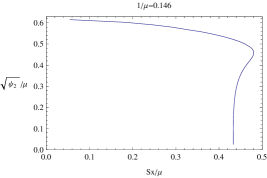
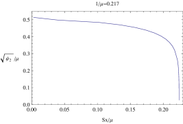
Figure 1: The phase structures in the case of nonzero $A_{x}$.

In the left panel of Fig.1, we observe that there is a metastable region typical in the first order phase transitions. This metable region also appeared in the St$\ddot{u}$ckelberg mechanism for the first order phase transition S. Franco ; Q.Y. Pan-1 . In this region, the scalar field has different behavior in the condensation. $\psi_{2}$ at the horizon decreases with the decrease of $S_{x}/\mu$, instead of increasing when $S_{x}/\mu$ becomes smaller as in the normal condensates. In the upper panel of Fig.2 we delimit this difference. When we use the alternative quantization, i.e. by setting $\psi_{2}=0$, the difference also holds in $\psi_{1}$ as shown in the lower panel of Fig.2.

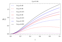
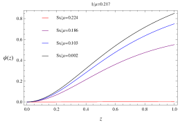
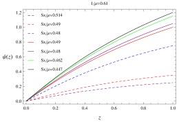
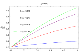
Figure 2: The evolution of scalar field. The solid lines are for the stable hairy phases while the dashed lines correspond to the metastable states. The two figures in the upper panel are for taking $\psi_{1}=0$ while those in the lower panel are for setting $\psi_{2}=0$.

In the following we will discuss the aspects of the conductivity and examine the behaviors of conductivity for the first order and the second order phase transitions. We will only concentrate on the transverse conductivity here for simplicity and solve the transverse gauge field perturbation $\delta A_{y}=e^{-iwt}A_{y}$ numerically in the background with the condensate. The equation of motion for $A_{y}$ is

$$A_{y}^{{}^{\prime\prime}}+(\frac{2}{z}+\frac{f^{\prime}}{f})A_{y}^{{}^{\prime}}+(\frac{\omega^{2}}{f^{2}z^{4}}-\frac{2\psi^{2}}{z^{4}f})A_{y}=0.$$ (8)

This equation can be solved by imposing the ingoing boundary condition at the horizon for causality. At the boundary $A_{y}=A_{y}^{(0)}+A_{y}^{(1)}z+\cdots$. According to the linear response theory, the conductivity can be defined in terms of the retarded current-current correlators. The conductivity can be expressed as

$$\sigma_{y}(\omega)=\frac{A_{y}^{(1)}}{i\omega A_{y}^{(0)}}.$$ (9)

In Fig.3, we plot $Re[\sigma_{y}]$ for the operator $\mathbb{O}_{2}$. The solid lines correspond to the second order phase transition while the dashed lines are for the first order phase transition. Similar to that observed in the five dimensional situation P. Basu-1 , in our four dimensional case we observe that there is a conductivity gap for the first order phase transition while the gap disappears for the second order phase transition for the same $S_{x}/S_{xci}(i=1,2)$ both with $m^{2}=-2$ and $m^{2}=0$. We can understand the nonzero conductivity gap for the first order phase transition from two aspects. One is from the perturbation equation (8), we see that the profile of the scalar field imprints on the conductivity. Different profile of the field caused by different temperature and superfluid velocity shown in Fig.2 leads to different property in conductivity. The other is from the boundary side, the nonzero gap for the first order phase may attribute to the release or absorption of latent heat which accompany the first order transitionBinder . The existence of the conductivity gap for the first order phase transition means that the condensate has a binding energy, however for the second order phase transition the condensate can have arbitrarily low binding energyP. Basu-1 .

Furthermore we observe that the coherence peak for the first order phase transition is higher than that for the second order phase transition. The difference in the coherence peak is clearer for taking $m^{2}=0$. Since the coherence peak is controlled by the thermal fluctuations of the condensate Horbach , this actually shows that for the first order phase transition, the fluctuations are stronger. In other words, higher coherence peak for the first order phase transition indicates that only strong enough thermal fluctuations can induce the first order transition. Thus the superfluid velocity and the mass of the scalar field controls the strength of fluctuations in the system and the strength of the coherence peak can provide an effective description of different orders of phase transitions.

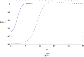
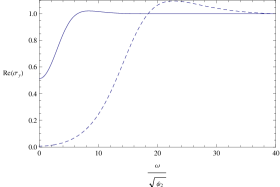
Figure 3: The transverse conductivity as a function of $\omega$ for $m^{2}=-2$(left) and $m^{2}=0$(right). The dashed lines are for the first order transition . The solid lines are for the second order transition.

Now we turn to discuss the susceptibility. In K. Maeda ; YQ Liu-1 , it was found that the susceptibility can be an effective tool to probe the holographic superconductivity. In condensed matter physics, the dynamical pair susceptibility can be measured directly via the second order Josephson effect and it is believed that this quantity can give direct view on the origin of the superconductivity She . We expect that the susceptibility can be a clear probe to identify the order of the phase transition in the holographic condensation.

In the dictionary of the AdS/CFT correspondence, the dynamical susceptibility in the boundary field theory can be calculated from the dynamics of the fluctuations of the corresponding scalar field in the bulk AdS background in the gravity side. We can expand the scalar perturbation as $\Psi=\psi(z)e^{-i\omega t}$. The equation of motion for the scalar field reads

$$\psi^{{}^{\prime\prime}}(z)+\frac{f^{\prime}}{f}\psi^{{}^{\prime}}(z)+\Big{[}\frac{(\omega+A_{t})^{2}}{f^{2}z^{4}}-\frac{(A_{x})^{2}}{fz^{2}}+\frac{2}{fz^{4}}\Big{]}\psi(z)=0.$$ (10)

Note that when $\omega=0$, the equation of motion (10) goes back to the third equation of (Observing various phase transitions in the holographic model of superfluidity). Eq.(10) can be solved by imposing the infalling boundary condition at the horizon

$$\psi\simeq(1-z)^{(-i\omega/4\pi T)}[1+\psi^{(1)}(1-z)+\psi^{(2)}(1-z)^{2}+\cdots].$$ (11)

Near the AdS boundary, the behavior of $\psi$ is still $\psi=z\psi_{1}+z^{2}\psi_{2}+\cdots.$ We choose $\psi_{1}$ as the source and $\psi_{2}$ as the response, then the dynamical pair susceptibility can be obtained as Son ; KW

$$\chi=G^{R}\sim\frac{\psi_{2}}{\psi_{1}}.$$ (12)

In the condensed matter physics, the imaginary part of this quantity can be measured via second order Josephson effect and is proportional to the current through a tunneling junction She .

The numerical results of the imaginary part of the dynamical pair susceptibility calculated in our gravity background as a function of the frequency $\omega$ are shown in Fig.4. We observe that when the fluid velocity decreases and approaches the transition point from the normal state to the superconducting state, the peak of the $\chi^{\prime\prime}$ becomes narrower and stronger. Comparing the imaginary part of the dynamical pair susceptibility exhibited in Fig.4, we find that for the first order phase transition the peaks of $\chi^{\prime\prime}$ are narrower than those of the second order phase transition for the same fluid velocity deviations from the critical moment. The peaks of $\chi^{\prime\prime}$ grow more violently for the first order phase transition, which approximate five times of the corresponding peaks in the second order phase transition for the same fluid velocity deviation from the critical value. These properties also hold when we look at the real part of the dynamical pair susceptibility.

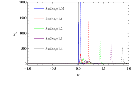
Figure 4: The imaginary part of the dynamical pair susceptibility. The solid lines are for the second order phase transition by taking $\frac{1}{\mu}=0.217$. The dashed lines are for the first order phase transition by taking $\frac{1}{\mu}=0.146$. The ratio of the fluid velocity to its critical value from right to left are $1.4$, $1.3$, $1.2$, $1.1$ and $1.02$ for the second and first order transitions.

In addition, the static pair susceptibility $\chi$ for $\omega=0$ can be obtained via Kramers-Kronig relation

$$\chi|_{\omega=0}=\frac{1}{\pi}\mathcal{P}\int_{-\infty}^{+\infty}\frac{\chi^{\prime\prime}(\omega^{\prime})}{\omega^{\prime}}d\omega^{\prime}.$$ (13)

It was argued that the static susceptibility can be an effective way to reflect the critical behavior near the condensationYQ Liu-1 . In the gravity side, to study $\chi|_{\omega=0}$, we can numerically solve (10) by setting $\omega=0$. In Fig.5 we plot the inverse of the static susceptibility with the change of the ratio of the fluid velocity to its critical value. The squares are for the first order phase transition with $1/\mu=0.146$, while the dots are for the second order phase transition with $1/\mu=0.217$. It is clear that the slope for the inverse static pair susceptibility becomes steeper near the first order phase transition than that near the second order phase transition. This also confirms that the first order phase transition has more violent phenomenon than the second order phase transition.

Thus we find that in studying the holographic superconductor in the AdS black hole background, both the conductivity and the pair susceptibility can be helpful to distinguish the order of the phase transition.

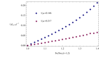
Figure 5: The behaviors of the static pair susceptibility for the first order phase transition and the second order phase transition. We set $m^{2}=-2$ in the computation.

In the following we extend our discussion to the AdS soliton background. The soliton spacetime is described by

$$ds^{2}=\frac{dr^{2}}{f(r)}+r^{2}(-dt^{2}+dx^{2})+f(r)d\eta^{2}$$ (14)

with $f(r)=r^{2}-\frac{r_{0}^{3}}{r}$. There is no horizon but a tip at $r_{0}$. We assume the matter fields are described by the lagrangian (1), where the vector field and the scalar field are in the form $A_{\mu}=A_{t}(r)dt+A_{\eta}(r)d\eta,\Psi=\Psi(r)$ Y. Brihaye . The investigation on other ansatz on the field of matters also can be seen in Montull1 ; Montull2 .

In the probe limit, the equations of motions of the matter fields in the AdS soliton background are described by

$$\psi^{{}^{\prime\prime}}+(\frac{f^{\prime}}{f}+\frac{2}{r})\psi^{{}^{\prime}}+\Big{[}\frac{A_{t}^{2}}{fr^{2}}-\frac{A_{\eta}^{2}}{f^{2}}-\frac{m^{2}}{f}\Big{]}\psi=0,$$

$$A_{t}^{{}^{\prime\prime}}+\frac{f^{\prime}}{f}A_{t}^{{}^{\prime}}-\frac{2\psi^{2}}{f}A_{t}=0,$$

$$A_{\eta}^{{}^{\prime\prime}}+\frac{2}{r}A_{\eta}^{{}^{\prime}}-\frac{2\psi^{2}}{f}A_{\eta}=0,$$ (15)

where the prime denotes the derivative with respect to $r$.

At the tip $r=r_{0}$, the fields have the asymptotic behavior:

$$\psi = U+V(r-r_{0})+W(r-r_{0})^{2}\cdots,$$

$$A_{t} = M+N(r-r_{0})+P(r-r_{0})^{2}\cdots,$$

$$A_{\eta} = a(r-r_{0})+b(r-r_{0})^{2}\cdots.$$ (16)

While near the AdS boundary the fields behave similarly to that in the black hole background,

$$\psi = \frac{\psi_{1}}{r}+\frac{\psi_{2}}{r^{2}},$$

$$A_{t} = \mu-\rho/r,$$

$$A_{\eta} = S_{\eta}-J_{\eta}/r.$$ (17)

In order to compare the results with those in the black hole, in our numerical computation we still set $m^{2}=-2$ and $r_{0}=1$.

In Fig.6 we plot the condensation of the operator $\mathbb{O}_{2}$ in the AdS Soliton background for different values of $1/\mu$. It is different from that we observed in the AdS black hole background, the condensates drop to zero continuously at critical values of the fluid velocity. There is always second order phase transition in the AdS soliton background when the normal state changes to the superconducting state. In the AdS black hole case, we know that the first order phase transition was brought by introducing the spatial dependence of the vector potential and the first order structure to the superconducting state appears at low temperature as the fluid velocity is increased. However, in the AdS soliton case, the spatial dependence of the vector potential $A_{\eta}$ is not countable to accommodate the first order phase transition, because it behaves like $A_{t}$ in the AdS black hole case. This can be easily seen by changing $r=1/z$ in the third equation of (Observing various phase transitions in the holographic model of superfluidity). In the AdS soliton, the first order phase transition can not exist in the probe limit, it can be brought only when we take account of the strong backreaction Gary T or in the St$\ddot{u}$ckelberg mechanism [42]. When we increase the values of $1/\mu$ from $1/8$, $1/5$ to $1/3$, the critical values of $S_{\eta}/\mu$ to start the condensation also increase from $1.241$, $1.279$ to $2.641$. This is a special character in the AdS soliton.

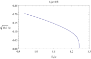
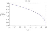
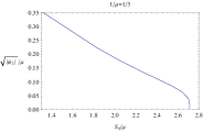
Figure 6: The condensates of the scalar operator $\mathbb{O}_{2}$ with respect to $S_{\eta}/\mu$ for chosen values of $1/\mu$.

We can calculate the conductivity $\sigma_{x}$ when we have the spatial dependence of the vector potential in the AdS soliton background. Considering the electromagnetic perturbation $\delta A_{x}=e^{-i\omega t}A_{x}$ in the bulk, we have the equation of motion for $A_{x}$

$$A_{x}^{{}^{\prime\prime}}+\frac{f^{\prime}}{f}A_{x}^{{}^{\prime}}+(\frac{\omega^{2}}{fr^{2}}-\frac{2\psi^{2}}{f})A_{x}=0.$$ (18)

At the tip, $A_{x}$ behaves as

$$A_{x}=aa+bb(r-r_{0})+cc(r-r_{0})^{2}\cdots.$$ (19)

While near the boundary

$$A_{x}=A_{x}^{(0)}+\frac{A_{x}^{(1)}}{r}+\cdots.$$ (20)

The behavior of the conductivity $\sigma_{x}(\omega)=\frac{A_{x}^{(1)}}{i\omega A_{x}^{(0)}}$ is shown in Fig.7. The left panel is for the AdS soliton before condensation while the right panel is after the condensation.

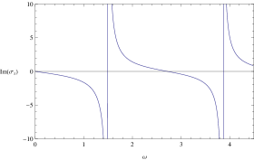
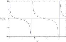
Figure 7: The imaginary part of the conductivity for the AdS soliton.

The behavior of the conductivity in the AdS soliton background presented here is similar to the result when we did not consider the spatial dependence of the vector potential in Q.Y. Pan-2 .

Furthermore we go on to study the pair susceptibility in the AdS soliton background. Similarly, taking $\Psi=\psi(r)e^{-i\omega t}$, the scalar perturbation equation reads

$$\psi^{\prime\prime}+(\frac{f^{\prime}}{f}+\frac{2}{r})\psi^{\prime}+[\frac{(A_{t}+\omega)^{2}}{fr^{2}}-\frac{A_{\eta}^{2}}{f^{2}}-\frac{m^{2}}{f}]\psi=0.$$ (21)

The asymptotic behavior near the boundary $r\rightarrow\infty$ is still $\psi=\frac{\psi_{1}}{r}+\frac{\psi_{2}}{r^{2}}+\cdots$. Beginning with (21), we can find that the scalar field behaves as

$$\psi\simeq(r-r_{0})^{|A_{\eta}|/3}[1+U(r-r_{0})+V(r-r_{0})^{2}+\cdots]$$ (22)

at the soliton rip. It is interesting that in the AdS soliton case, there is no imaginary part of the dynamical pair susceptibility, only the real part of pair susceptibility exists as shown in Fig.8 for the operator $\mathbb{O}_{2}$. The vanish of the imaginary part of the dynamical pair susceptibility can be attributed to the fact that both (21) and (22) are real.

Different from that in the AdS black hole, in the AdS soliton case we observe that the real part of the dynamical pair susceptibility is similar to the description of the BCS pair instability F. Marsiglio . With the change of $1/\mu$, we also observe the move of the curve with the horizontal line up and down. This is similar to the effect of the temperature in the description of the BCS pair instability which is the key factor to characterize the stability. However this is just a phenomenological similarity at the first sight, whether there is further deep connection still needs careful study.

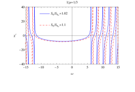
Figure 8: (color online) The real part of the pair susceptibility for operators $\mathbb{O}_{2}$.

In conclusion, we have studied the gravity duals of supercurrent solutions with general phase structure to describe both the first and the second order phase transitions at finite temperature in strongly interacting systems. We have argued that the conductivity and the pair susceptibility, which are measurable quantities in the condensed matter physics, can be possible phenomenological indications to distinguish the order of phase transitions. Besides the AdS black hole background, we have also extended our discussion to the AdS soliton configuration. We have found that in the AdS soliton, the first order phase transition cannot be brought by the supercurrent. The conductivity behaves similar to the case when there is only electric field $A_{t}$. There is no imaginary part of the dynamical pair susceptibility and the real part of the pair susceptibility behaves similar to that disclosed in the BCS pair instability F. Marsiglio . Further understanding on this phenomenological similarity is called for.

- (1) J. M. Maldacena, Adv. Theor. Math. Phys. 2, 231 (1998).
- (2) S. S. Gubser, I. R. Klebanov and A. M. Polyakov, Adv. Theor. Math. Phys. Lett.B 428, 105 (1998).
- (3) E. Witten, Adv. Theor. Math. Phys. 2, 253 (1998).
- (4) S.A. Hartnoll, Class. Quant. Grav. 26, 224002 (2009).
- (5) C.P. Herzog, J. Phys. A 42, 343001 (2009).
- (6) G.T. Horowitz, arXiv:1002.1722 [hep-th].
- (7) G.T. Horowitz and M.M. Roberts, Phys. Rev. D 78, 126008 (2008).
- (8) S.A. Hartnoll, C.P. Herzog, and G.T. Horowitz, Phys. Rev. Lett. 101, 031601 (2008).
- (9) E. Nakano, W.Y. Wen, Phys. Rev. D 78, 046004 (2008).
- (10) I. Amado, M. Kaminski, and K. Landsteiner, J. High Energy Phys. 0905, 021 (2009).
- (11) G. Koutsoumbas, E. Papantonopoulos, and G. Siopsis, J. High Energy Phys. 0907, 026 (2009).
- (12) O.C. Umeh, J. High Energy Phys. 0908, 062 (2009).
- (13) H.B. Zeng, Z.Y. Fan, and Z.Z. Ren, Phys. Rev. D 80, 066001 (2009).
- (14) J. Sonner, Phys. Rev. D 80, 084031 (2009).
- (15) S.S. Gubser, C.P. Herzog, S.S. Pufu, and T. Tesileanu, Phys. Rev. Lett. 103, 141601 (2009).
- (16) J.P. Gauntlett, J. Sonner, and T. Wiseman, Phys. Rev. Lett. 103, 151601 (2009).
- (17) R.G. Cai and H.Q. Zhang, Phys. Rev. D 81, 066003 (2010).
- (18) J.L. Jing and S.B. Chen, Phys. Lett. B 686, 68 (2010).
- (19) C.P. Herzog, Phys. Rev. D 81, 126009 (2010).
- (20) S.B. Chen, L.C. Wang, C.K. Ding, and J.L. Jing, Nucl. Phys. B 836, 222 (2010).
- (21) R.A. Konoplya and A. Zhidenko, Phys. Lett. B 686, 199 (2010).
- (22) J.P. Wu, Y. Cao, X. M. Kuang, W. J. Li, Phys. Lett. B 697, 153-158 (2011).
- (23) G. Siopsis and J. Therrien, J. High Energy Phys. 1005, 013 (2010).
- (24) K. Maeda, M. Natsuume, and T. Okamura, Phys. Rev. D 79, 126004 (2009).
- (25) R. Gregory, S. Kanno, and J. Soda, J. High Energy Phys. 0910, 010 (2009).
- (26) Q.Y. Pan, B. Wang, E. Papantonopoulos, J. Oliveira, and A.B. Pavan, Phys. Rev. D 81, 106007 (2010).
- (27) X.H. Ge, B. Wang, S.F. Wu, and G.H. Yang, J. High Energy Phys. 1008, 108 (2010).
- (28) X. He, B. Wang, R.G. Cai, and C.Y. Lin, Phys. Lett. B 688, 230 (2010).
- (29) R.G. Cai, Z.X. Nie, B. Wang, and H.Q. Zhang, arXiv:1005.1233 [gr-qc].
- (30) X.M. Kuang, W.J. Li and Y. Ling, J. High Energy Phys. 1012, 069 (2010).
- (31) A. Akhavana, M. Alishahiha, Rev. D 83, 086003 (2011)
- (32) Y. Brihaye and B. Hartmann, Phys. Rev. D 83, 126008 (2010).
- (33) S.S. Gubser, Phys. Rev. D 78, 065034 (2008).
- (34) S. A. Hartnoll, C. P. Herzog, and G. T. Horowitz, J. High Energy Phys. 0812 ,015 (2008).
- (35) S. Franco, A.M. Garcia-Garcia, and D. Rodriguez-Gomez, J. High Energy Phys. 1004, 092 (2010).
- (36) S. Franco, A.M. Garcia-Garcia, and D. Rodriguez-Gomez, Phys. Rev. D 81, 041901(R) (2010).
- (37) F.Aprile and J.G. Russo, Phys. Rev. D 81, 026009 (2010).
- (38) Q.Y. Pan and B. Wang, Phys. Lett. B 693, 159 (2010).
- (39) Y.Q. Liu, Q.Y. Pan and B. Wang, Phys. Lett. B 702 94-99 (2011).
- (40) T. Nishiokaa,S. Ryu and T. Takayanagi, J. High Energy Phys. 1003, 131 (2010).
- (41) G. T.Horowitz, B. Way, J. High Energy Phys. 1011, 011 (2010) .
- (42) P. Yan, Q.Y.Pan, B.Wang, Phys. Lett. B 699 (5) (2011).
- (43) N. Bobev, A. Kundu, K. Pilch, N. P. Warner, JHEP 1203 (2012) 064.
- (44) C. Herzog, P. Kovtun and D. Son, Phys. Rev. D 79, 066002 (2009).
- (45) P. Basu, A. Mukherjee and H. H. Shieh, Phys. Rev. D 79, 045010(2009).
- (46) J. Sonner and B. Withers, Phys. Rev. D 82, 026001(2010).
- (47) D. Arean, M. Bertolini, J. Evslin, T. Prochazka, JHEP 1007:060,2010.
- (48) D. Arean, P. Basu and C. Krishnan, J. High Energy Phys. 10, 006 (2010).
- (49) K. Binder, Rep. Prog. Phys. 50 (1987) 783-859.
- (50) M. L. Horbach et al., Phys. Rev. B 46, 432 (1992); K. Holczer et al., Phys. Rev. Lett. 67, 152 (1991).
- (51) K. Maeda, M. Natsuume, T. Okamura, Phys.Rev.D79, 126004 (2009).
- (52) Y.Q. Liu, Q.Y. Pan, B. Wang, R.G. Cai, Phys. Lett B, 693(3) (2010).
- (53) J.H. She, B. J. Overbosch, Y. W. Sun, Y. Liu, K. Schalm, J. A. Mydosh and J. Zaanen, Phys. Rev. B 84, 144527 (2011).
- (54) D. T. Son and A. O. Starinets, J. High Energy Phys.0209, 042 (2002).
- (55) I. R. Klebanov and E. Witten, Nucl. Phys. B 556, 89 (1999).
- (56) M. Montull, O. Pujolas, A. Salvio, P. J. Silva, Phys.Rev.Lett. 107 (2011) 181601
- (57) M. Montull, O. Pujolas, A. Salvio, P. J. Silva, JHEP 1204 (2012) 135
- (58) F. Marsiglio, K. S. D. Beach, and R. J. Gooding, [arXiv:1203.5122[cond-mat]].