Calibration of Nonthermal Pressure in Global Dark Matter Simulations of Clusters of Galaxies

Abstract

We present a new method for incorporating nonthermal pressure from bulk motions of gas into an analytic model of the intracluster medium in clusters of galaxies, which is based on a polytropic equation of state and hydrostatic equilibrium inside gravitational potential wells drawn from cosmological dark matter simulations. The pressure is allowed to have thermal and nonthermal components with different radial distributions; the overall level of nonthermal support is based on the dynamical state of the halo, such that it is lower in more relaxed clusters. This level is normalized by comparison to pressure profiles derived from X-ray observations, and to a high resolution hydrodynamical simulation. The nonthermal pressure fraction measured at $r_{500}$ is typically in the range 10-20%, increasing with cluster mass and with redshift. The resulting model cluster properties are in accord with Sunyaev-Zel’dovich (SZ) effect observations of clusters. Inclusion of nonthermal pressure reduces the expected angular power spectrum of SZ fluctuations in the microwave sky by 24%.

1 Introduction

The millimeter and microwave sky has recently been mapped on small angular scales to much higher precision than was previously possible, most notably by the South Pole Telescope (SPT Lueker et al., 2010; Shirokoff et al., 2011; Reichardt et al., 2011) and the Atacama Cosmology Telescope (ACT Fowler et al., 2010; Das et al., 2011). These telescopes, as well as the PLANCK satellite, will soon provide further results with increased frequency and sky coverage. At these scales (multipoles $\ell\gtrsim 3000$) the primordial cosmic microwave background is strongly damped, and other components dominate. After accounting for point sources, such as dusty star forming galaxies and radio galaxies (Hall et al., 2010; Vieira et al., 2010; Marriage et al., 2011), the main contributor to microwave anisotropies is then the Sunyaev-Zel’dovich (SZ) effect from galaxy clusters, groups, and the intergalactic medium. SZ measurements can give strong constraints on cosmological parameters (e.g. Komatsu et al., 2011; Das et al., 2011; Dunkley et al., 2010; Sehgal et al., 2011; Reichardt et al., 2011), particularly the normalization of the matter power spectrum, conventionally given as $\sigma_{8}$, the amplitude of fluctuations on an 8$h^{-1}$Mpc scale.

However, these constraints rely on the ability to predict the SZ signal for a given set of cosmological parameters. This requires knowledge of the state of the intracluster medium (ICM) in groups and clusters out to high redshift. Many physical processes shape the ICM, including shocks from accretion and merging, star formation, supernovae, and active galactic nuclei (AGN), among others. Our understanding of these processes and their effect on the ICM over time is still evolving. Measurements of how the relations among X-ray and SZ observables (and their relation to mass) evolve with redshift are ongoing; current observational constraints at higher $z$ leave much room for improvement (Reichert et al., 2011). On the theoretical side, lacking analytic solutions for gravitational collapse and many aspects of the behavior of baryons, recourse is taken to numerical simulations. Full hydrodynamic simulations with all the required physical inputs are expensive to run and involve many details of subgrid physics; different numerical schemes can give varying results (Agertz et al., 2007; Mitchell et al., 2009; Vazza et al., 2011b; Sijacki et al., 2011). Thus, global predictions of the expected SZ signal are currently highly uncertain.

With this in mind, we have developed a method for determining the ICM distribution in a given gravitational potential well (Ostriker et al., 2005; Bode et al., 2007, 2009; Trac et al., 2011). This makes it possible to take the output of a large volume cosmological simulation with only dark matter (DM) and, by populating the halos with gas, produce predictions for the SZ signal over a large area of the sky. To date, this model has assumed that the gas is in hydrostatic equilibrium (HE) and that it has a polytropic equation of state. Levels of star formation and feedback energy are set so that the model matches current X-ray observations. Based on this, the “Standard” model of Bode et al. (2009, hereafter BOV09) was used to produce an all-sky SZ map (Sehgal et al., 2010); this yields a template for the angular power spectrum which can be compared with microwave observations. SPT (Lueker et al., 2010; Shirokoff et al., 2011; Reichardt et al., 2011) and ACT (Fowler et al., 2010; Dunkley et al., 2010) both found that the observed power is lower (by up to a factor of 2) than expected from this template. A possible explanation for this discrepancy is that the BOV09 model overestimates the thermal pressure in the outer regions of clusters. X-ray scalings, to which the model is normalized, are generally not measured beyond $r_{500}$ (the radius within which the cluster density is 500 times the critical value) because this region dominates the signal, whereas the SZ angular power spectrum is significantly affected by the regions outside this radius.

In particular, bulk motions of gas and turbulent pressure support will occur, making the assumption of HE incorrect. This would be more likely in the outer regions of clusters, where the gas has been accreted more recently, and in younger, less dynamically relaxed clusters. There is considerable support from simulations for this picture, with the temperature dropping below that which would be predicted by HE (Lau et al., 2009; Burns et al., 2010; Vazza et al., 2011a; Battaglia et al., 2011a). Though difficult to obtain, there is some observational evidence that nonthermal sources of pressure are present in cluster outskirts. Drops in the average temperature with radius, leading to a flattening in the radial profile of entropy, have been seen (Mahdavi et al., 2008; George et al., 2009; Bautz et al., 2009; Hoshino et al., 2010; Urban et al., 2011; Akamatsu et al., 2011; Morandi et al., 2011), although this is not always the case (Reiprich et al., 2009; Ettori & Balestra, 2009; Simionescu et al., 2011; Humphrey et al., 2012). Gas clumping (Simionescu et al., 2011; Urban et al., 2011), deviations from symmetry (Eckert et al., 2011b; Walker et al., 2012), and the fact that backgrounds dominate (Eckert et al., 2011a) complicate interpretation of these observations.

Trac et al. (2011) included nonthermal pressure in the polytropic model, and found the resulting SZ template significantly reduced the tension with current SZ measurements. However, this had the limitation of assuming that the fraction of nonthermal pressure was the same (20%) at all radii, and the same for all cluster masses and redshifts, when in fact physical modeling indicates that the nonthermal fraction should be larger in the outer parts of clusters, and should also be larger in recently formed clusters (i.e. increase with increasing redshift).

The assumption of a polytropic equation of state means the gas density is given by $\rho=\rho_{0}\theta^{\frac{1}{\Gamma-1}}$ and the pressure by $P=P_{0}\theta^{\frac{\Gamma}{\Gamma-1}}$, where the polytropic variable $\theta$ is a function of the potential, the central density $\rho_{0}$, and the central pressure $P_{0}$ (see Eqn. 1). Based on hydrodynamical simulations of cluster formation, Ostriker et al. (2005) assumed $P$ represented thermal pressure only, and argued that the appropriate polytropic index was $\Gamma=1.2$. Shaw et al. (2010, hereafter SNBL), based on more recent simulations, instead argued that it is the sum of thermal and turbulent pressures which follows the polytropic relation (but still with $\Gamma=1.2$). In this case the fraction of nonthermal pressure varies within a cluster, increasing with radius, and also increases with redshift. The simulations of Battaglia et al. (2011a) give support for a cluster mass dependence as well.

In this paper we modify the model of BOV09 to include a treatment of nonthermal pressure similar to that presented in SNBL. Our approach will differ from SNBL in that it will be based on the dynamical state of each individual halo, such that less relaxed halos have a higher level of turbulent pressure. The relation between the level of virialization and the fraction of turbulent pressure is calibrated by comparison to cosmological hydrodynamic simulations (in particular a high resolution run using the ENZO code) and the pressure profile derived from X-ray observations.

Sec. 2 summarizes the polytropic model. Sec. 3 presents the new method for including turbulent pressure, which includes a free parameter that is set by normalizing to observed and simulated clusters. Note the model parameters are set by comparison to X-ray data only. The model, applied to a large set of halos, is then compared to SZ observations in Sec. 4.

2 Polytropic Model

The goal behind this work is, given a particular cosmology, to produce a simulated map of the microwave sky. The strategy is to first run a pure dark matter simulation of a large volume, saving the mass distribution along the past light cone. The group and cluster sized halos in the light cone are identified, and each in turn is populated with gas; thus the thermal and kinetic SZ effect arising from clusters can be calculated. In this paper we will use halo samples drawn from a light cone output of a simulated cube 1000 $h^{-1}$Mpc on a side (see BOV09 for more details) with cosmological parameters ($\Omega_{b},\Omega_{m},\Omega_{\Lambda},h,n_{s},\sigma_{8}$) = (0.044, 0.264, 0.736, 0.71, 0.96, 0.80), consistent with the WMAP 7-year results (Komatsu et al., 2011).

Adding gas to halos is done with the method of BOV09. Gas is placed in the DM gravitational potential $\phi$ such that it is in hydrostatic equilibrium and has a polytropic equation of state. The polytropic variable $\theta$ is

$$\theta\equiv 1+\frac{\Gamma-1}{\Gamma}\frac{\rho_{0}}{P_{0}}\left(\phi_{0}-\phi\right)\;,$$ (1)

where $\phi_{0}$, $\rho_{0}$, and $P_{0}$ are the central values at radius $r=0$. BOV09 assumed that $P_{0}$ was due to thermal pressure alone. Here we will instead follow SNBL, so that it is the sum of thermal and turbulent pressures which follows the polytropic relation. The turbulent component will have the same compressibility as the thermal component, so the polytropic index remains $\Gamma=1.2$. Thus the total pressure is the sum of thermal $P_{th}$ and turbulent $P_{nth}$ components:

$$P=P_{th}+P_{nth}=P_{0}\theta^{\frac{\Gamma}{\Gamma-1}}\hskip 28.45274pt,$$ (2)

$$f_{nth}=P_{nth}/(P_{th}+P_{nth})\hskip 28.45274pt,$$ (3)

$$P_{th}=(1-f_{nth})P_{0}\theta^{\frac{\Gamma}{\Gamma-1}}\hskip 28.45274pt.$$ (4)

The density profile is unchanged from BOV09, but the temperature is altered by a factor $(1-f_{nth})$. $f_{nth}$ varies with radius, so the effective polytropic index, $\Gamma_{eff}=d\log P_{th}/d\log\rho$ is not constant, but rather increases with radius. We will let $f_{nth}$ also vary with cluster mass and redshift (see Sec. 3).

Two constraints are used to fix the central values $\rho_{0}$ and $P_{0}$ (see BOV09, ). First, the total pressure at the outer radius must match the surface pressure $P_{s}$ (calculated from the DM in a buffer region at $r_{vir}$). Second, energy must be conserved. Assume the gas initially followed the DM density distribution inside the virial radius $r_{vir}$, with the same specific energy. Some of the gas (that with the lowest entropy) is removed and placed into stars. The remaining gas has an initial energy $E_{g}$; this gas is now rearranged to obey the polytropic equation of state. The energy of the gas in this final arrangement is $E_{f}=\frac{3}{2}\int PdV$ (the integral is over the cluster volume, out to the outermost extent of the rearranged gas, $r_{f}$; note $r_{f}$ can be larger than $r_{vir}$). This energy must equal the initial value, modified by various processes (see BOV09 for details):

$$E_{f}=E_{g}+\Delta E_{P}+\epsilon_{D}\left|E_{D}\right|+\epsilon_{F}M_{*}c^{2}\hskip 28.45274pt.$$ (5)

The first modification to the initial gas energy is a change due to expansion (or contraction) of the gas, $\Delta E_{P}=(4\pi/3)(r_{vir}^{3}-r_{f}^{3})P_{s}$, which accounts for mechanical work done against the surface pressure. The next term is a dynamical energy input, needed because during cluster formation energy is transferred from DM to gas by dynamical processes (McCarthy et al., 2007). The binding energy $E_{D}$ of the DM is found, and 5% ($\epsilon_{D}=0.05$) is added to the gas; this value provides a good match to the gas fractions seen in “adiabatic” (no radiative cooling or star formation) hydrodynamic simulations (Crain et al., 2007; Young et al., 2011).

The final term in Eqn. 5 is feedback from star and black hole formation, where $M_{*}$ is the mass of stars inside the virial radius The mass in stars at $z=0$ is set to

$$M_{*}/M_{vir}=A_{*}\left(5.0\times 10^{13}M_{\odot}/M_{500}\right)^{\alpha_{*}}\;,$$ (6)

where $M_{500}$ and $M_{vir}$ are the total mass inside $r_{500}$ and $r_{vir}$, respectively. From the infrared properties of clusters, Lin et al. (2003) found $A_{*}=0.026$ and $\alpha_{*}=0.26$ when measuring the stellar mass inside $r_{500}$. For nearby, low-mass galaxy clusters, Balogh et al. (2011) find stellar fractions in agreement with Lin et al. (2003). Note we use these parameters to give $M_{*}$ for the entire cluster out to the virial radius (not just inside $r_{500}$); Andreon (2010) found that this choice gives a model that matches the observed stellar fraction within $r_{200}$. This stellar fraction differs (particularly at lower masses) from that found by Giodini et al. (2009), who obtained $A_{*}=0.05$ and $\alpha_{*}=0.37$ (again measuring inside $r_{500}$). However, we find that with the Lin et al. (2003) values the model clusters give a better match to observed electron pressure profiles (see Sec. 3). The redshift evolution of stellar mass, including gas recycling, is handled in the manner described in BOV09. Lin et al. (2012) find little evolution in the stellar fraction relative to Lin et al. (2003) out to $z\sim 0.6$. At higher redshifts ($\sim$0.2–1), and measuring out to 200 times the mean density, Leauthaud et al. (2011b) find total stellar fractions lower than what we are using here (see also Leauthaud et al., 2011a); adjusting for intra-cluster light would at least partially reduce the difference.

Feedback energy, from both supernovae and AGN, is parametrized as $\epsilon_{F}M_{*}c^{2}$. This will be set to match observations (Sec. 3.3); we find $\epsilon_{F}=8\times 10^{-6}$. If the mass in black holes is $\sim 10^{-3}M_{*}$, this means roughly $6\times 10^{-3}$ of the black hole rest mass is deposited in the surrounding gas (ignoring the supernova contribution). A similar value of $5\times 10^{-3}$ is needed in simulations to produce the correct relationship between black hole mass and stellar velocity dispersion (Di Matteo et al., 2005). If 15% of the baryons are turned into stars, then this level of feedback adds 1 keV per particle initially inside the virial radius; this is actually lower than the value of $2.62\pm 0.85$ keV per particle Chaudhuri et al. (2012) derived from X-ray data.

It is possible to include relativistic pressure, e.g. cosmic rays and tangled magnetic fields, under the assumption that relativistic contribution is proportional to the non-relativistic pressure, i.e. $P_{rel}=\delta_{rel}(P_{th}+P_{nth})$ (see Bode et al., 2009; Trac et al., 2011). However, we will not do so (in effect setting $\delta_{rel}=0$), because including this effect did not improve the fit to observed clusters.

3 Incorporating nonthermal pressure

3.1 Nonthermal pressure from turbulence and bulk motions

Based on adaptive mesh refinement hydrodynamic simulations of cluster formation (which include star formation and feedback), SNBL found that the radial profile of the nonthermal pressure fraction follows a power law in radius:

$$f_{nth}=\alpha\left(\frac{r}{r_{500}}\right)^{n_{nth}}\;\;,$$ (7)

with $n_{nth}=0.80\pm 0.25$. Examining their simulations out to $z=1$, SNBL derived a redshift-dependent normalization

$$\alpha(z)={\rm MIN}[\alpha_{0}(1+z)^{\beta},\;(4^{-n_{nth}}\alpha_{0}^{-1}-1)\tanh(\beta z)+1]\;\;,$$ (8)

where $\alpha_{0}=0.18\pm 0.06$ and $\beta=0.5$. Battaglia et al. (2011a) also used simulations to constrain $f_{nth}$, with clusters out to $z=1.5$ drawn from a set of smoothed particle hydrodynamics cosmological boxes; star formation and AGN feedback were included. They saw redshift evolution similar to SNBL, but also a weak mass dependence; for $z\lesssim 1$ this can be included by modifying $\alpha$ to be

$$\alpha(z,M)=\alpha_{0}(1+z)^{\beta}\left(\frac{M_{200}}{3\times 10^{14}M_{\odot})}\right)^{0.2}\;\;.$$ (9)

These results seem to be robust with regard to the details of the gas physics, as both SNBL and Battaglia et al. (2011a) obtain similar values when not including gas cooling and star formation.

This can easily be incorporated into the method of BOV09. One possibility is to simply use Eqn. 8 or 9 for $\alpha$. However, it is seen in simulations that relaxed clusters tend to have less turbulent pressure support than unrelaxed ones (Lau et al., 2009; Vazza et al., 2011a; Paul et al., 2011; Hallman & Jeltema, 2011; Nelson et al., 2011). Thus, rather than giving all halos at a given mass and redshift the same value for nonthermal fraction, it would be more accurate to base $\alpha$ on the dynamical state of the halo. We will do this as follows in the next section.

3.2 Setting the level of nonthermal pressure

The mean nonthermal energy fraction in the gas is given by $\bar{f}=\int P_{nth}dV/\int PdV$, with the integrals over the cluster volume out to the virial radius. In a situation where the density and temperature distribution of the gas is known (e.g. from an observed cluster or a hydrodynamical simulation), the fraction of energy due to turbulent nonthermal pressure can be computed directly as

$$\bar{f}=\frac{\int\frac{1}{3}\rho\sigma^{2}dV}{\int\left(\frac{\rho kT}{\mu m_{p}}+\frac{1}{3}\rho\sigma^{2}\right)dV}\;,$$ (10)

where $\sigma^{2}$ is the velocity dispersion, $k$ is the Boltzmann constant, and $\mu m_{p}$ is the mean mass of the ICM particles.

When determining the polytropic gas distribution for a DM-only halo, the total pressure $P$ is found before determining the turbulent and thermal components separately. For a given cluster we can thus compute a measure $f^{\prime}_{pol}$ proportional to the nonthermal energy fraction $\bar{f}_{pol}$ when assuming the form of Eqn. 7:

$$\bar{f}_{pol}=\frac{\int\alpha(r/r_{500})^{n_{nth}}PdV}{\int PdV}=\alpha f^{\prime}_{pol}\;.$$ (11)

We wish to base the value of $\bar{f}=\alpha f^{\prime}_{pol}$ on the properties of the DM halo; thus a measure of how relaxed or disturbed a halo may be is required. The virial theorem states $\ddot{I}/2=2K+W-E_{S}$, where $K$ and $W$ are the kinetic and potential energies, $I$ is the moment of inertia, and $E_{S}$ is a surface pressure term (the surface is located at the virial radius $r_{vir}$). Thus for a DM halo in HE ($\ddot{I}=0$) we expect kinetic energy $K_{vt}=(E_{S}-W)/2$. Let us identify any variation from this as being due to an out of equilibrium state, which will also be reflected in turbulence. Then we can compute from the DM a measure of the degree to which the system is out of equilibrium:

$$\bar{f}_{neq}=\frac{|K-K_{vt}|}{K}=\left|\frac{2K}{E_{S}-W}-1\right|\;.$$ (12)

We will assume that the level of nonthermal support in the gas is proportional to this measure, or $\bar{f}=\kappa\bar{f}_{neq}$, where $\kappa$ is a constant independent of mass and redshift. Thus, limiting the thermal pressure to be less than the total at the outermost gas radius $r_{f}$ (i.e. $\alpha(r_{f}/r_{500})^{n_{nth}}\leq 1$), we have

$$\alpha={\rm MIN}\left[\;\kappa\bar{f}_{neq}/f^{\prime}_{pol},\;(r_{500}/r_{f})^{n_{nth}}\;\right]\;.$$ (13)

It only remains to set the constant of proportionality $\kappa$; once this is known, $P_{nth}$ and $P_{th}$ can be computed in the polytropic model. We will determine $\kappa$ in two ways: by matching the observed electron pressure at $r_{500}$, and by computing the thermal pressure directly from the gas in a simulated cluster which includes full hydrodynamics.

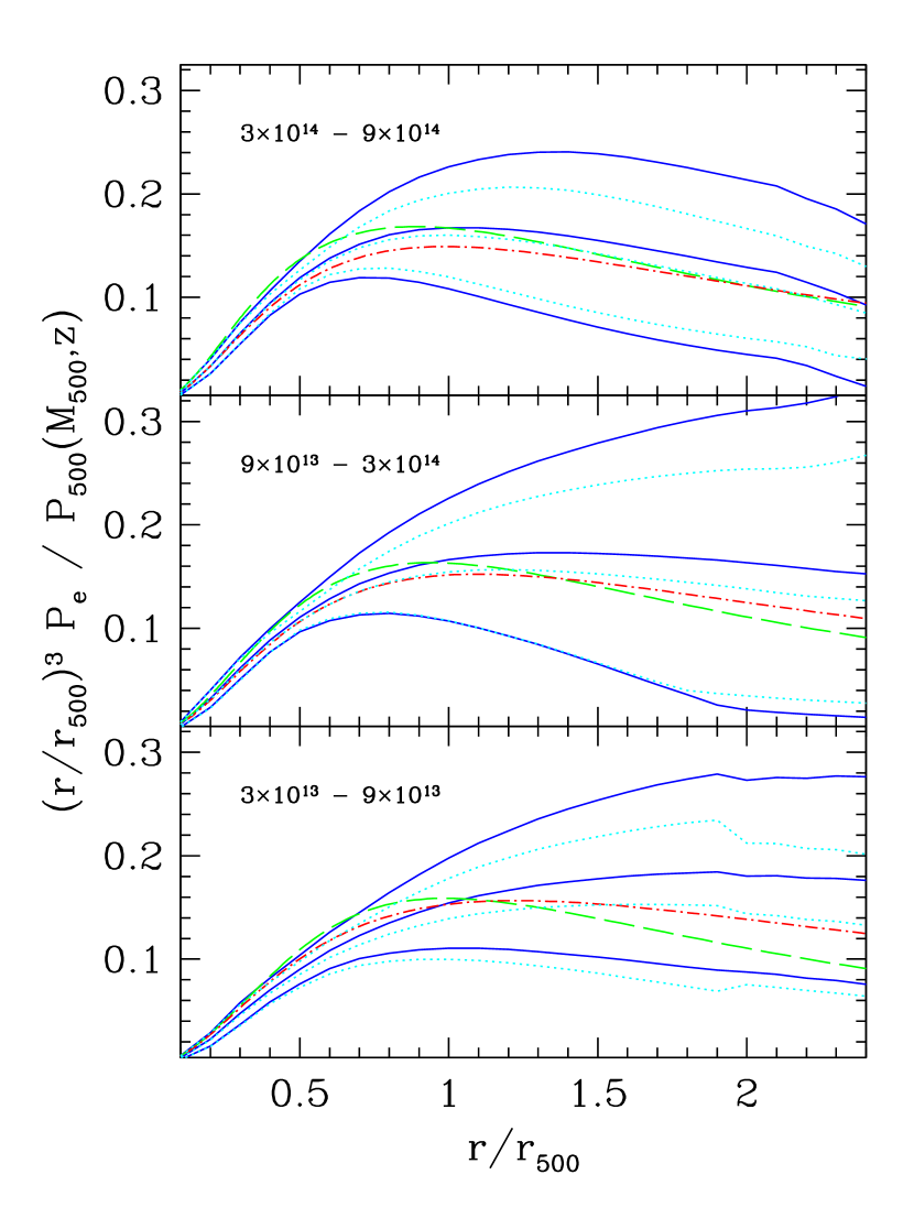
Figure 1: Electron pressure profiles of model clusters. Each panel is labeled by the mass range used; the mean redshift is $z\approx 0.1$. The dashed line is the universal profile from X-ray data by Arnaud et al. (2010), who give an expression for the normalization factor $P_{500}$. The solid lines indicate the mean and one standard deviation for the model clusters when basing $\alpha$ on the dynamics (Eqn. 13). The dotted lines instead use constant $\alpha_{0}=0.18$ in Eqn. 8, following SNBL. Dot-dashed lines are the mean simulated profile of Battaglia et al. (2011b), based on the mean $M_{200}$ and redshift of each bin.

From X-ray data, Arnaud et al. (2010) derived a electron pressure profile of low redshift clusters; Sun et al. (2011) found this same profile holds for local galaxy groups. This profile is shown as a dashed line in Fig. 1. Note that, due to the paucity of observations, outside of $r_{500}$ this profile is derived from simulations; also, for higher redshifts it assumes self-similar scaling. To compare the model profiles with this universal form, we divided a sample of low redshift ($z<0.2$) DM halos from the lightcone into three mass bins: $3\times 10^{13}\leq M_{500}/M_{\odot}<9\times 10^{13}$; $9\times 10^{13}\leq M_{500}/M_{\odot}<3\times 10^{14}$; and $3\times 10^{14}\leq M_{500}/M_{\odot}<9\times 10^{14}$. The mean pressure profile was calculated for each mass bin, and $\kappa$ was varied to minimize the difference between the observed and model profiles at $r_{500}$. For this purpose $P_{th}$ was converted to electron pressure and normalized by $P_{500}$ (Arnaud et al., 2010); the observed profile was calculated using the mean mass and redshift of the model halos in each bin. The best fit value is $\kappa=0.70$; the resulting profiles are shown as solid lines in Fig. 1 (the other parameters in the polytropic model are as listed in Sec. 2).

Steepening the radial dependence, by increasing $n_{nth}$ to as much as 1.2, did not produce a significantly improved match to the universal profile, so we leave $n_{nth}$ at the SNBL value of $0.8$. (It may be that $n_{nth}$ depends on how relaxed a cluster is; see Nelson et al. 2011). Cutting $\epsilon_{F}$ in half, to $4\times 10^{-6}$, also did not change the best fit $\kappa$. Note the outermost radius of the polytropic gas, $r_{f}$, varies from cluster to cluster. In most cases $r_{f}$ does not extend much beyond $2.6r_{500}$ for the high mass bin; this limit increases to $3.2r_{500}$ for the middle bin, while for the lowest mass bin it can extend to $4r_{500}$. The gas outside of $r_{f}$ needs to be treated separately when making SZ maps (Sehgal et al., 2010).

As an alternative method of fixing $\kappa$ (and thus the level of nonthermal pressure), we compare the resulting profile to that of a cluster taken from a hydrodynamical simulation (Cen, 2011) performed with an Eulerian adaptive mesh refinement code, Enzo (Bryan, 1999; Bryan & Norman, 1999; O’Shea et al., 2004; Joung et al., 2009). First a low resolution simulation with a periodic box of $120~{}h^{-1}$Mpc on a side was run, and a region centered on a cluster of mass of $\sim 2\times 10^{14}M_{\odot}$ was identified. We then resimulated this subbox with high resolution, but embedded in the outer $120h^{-1}$Mpc box in order to properly take into account the large-scale tidal field and the appropriate boundary conditions at the surface of the refined region. The subbox centered on the cluster has a size of $21\times 24\times 20h^{-3}$Mpc³. The initial conditions in the refined region have a mean interparticle separation of $117h^{-1}$kpc comoving and a dark matter particle mass of $1.07\times 10^{8}h^{-1}M_{\odot}$. The refined region is surrounded by two layers of buffer zones, each of $\sim 1h^{-1}$Mpc, with particle masses successively larger by a factor of $8$ for each layer; the outermost buffer then connects with the outer root grid, which has a dark matter particle mass $8^{3}$ times that in the refined region. The mesh refinement criterion is set such that the resolution is always better than $460h^{-1}$pc physical, corresponding to a maximum mesh refinement level of $11$ at $z=0$.

The cosmological parameters of the simulation are ($\Omega_{b},\Omega_{m},\Omega_{\Lambda},h,n_{s},\sigma_{8}$) = (0.046, 0.28, 0.72, 0.70, 0.96, 0.82). The simulation includes a metagalactic UV background (Haardt & Madau, 1996) and a model for shielding of UV radiation by neutral hydrogen (Cen et al., 2005). It also includes metallicity-dependent radiative cooling (Cen et al., 1995). Star particles are created in cells that satisfy a set of criteria for star formation proposed by Cen & Ostriker (1992); star particles typically have masses of $\sim$$10^{6}M_{\odot}$. Supernova feedback from star formation is modeled following Cen et al. (2005).

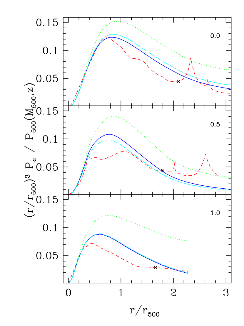
Figure 2: Comparison of radial profiles of electron pressure from a hydrodynamical simulation (red dashed lines) to the polytropic model applied to the DM potential. Each panel is labeled with the redshift. The $\times$ marks the virial radius. The dotted line is the model without nonthermal pressure. The solid line includes it, with $\kappa=0.7$ in Eqn. 13. The dot-dashed line instead uses the $\kappa$ parameter measured directly from the simulation at each redshift.

To emulate the manner in which the polytropic model is normally applied, the DM particles were taken from the halo at selected redshifts, and their masses were adjusted by a factor $(1+\Omega_{b}/\Omega_{DM})$ to account for the baryonic mass. These particles were then used as input to the polytropic model code. The assumed stellar fraction was increased to match that of the simulation, but feedback was not included (i.e. $\epsilon_{F}=0$) because the simulation did not include AGN. This cluster grows in mass from $M_{500}=4.1\times 10^{13}M_{\odot}$ at $z=1$ to $M_{500}=1.9\times 10^{14}M_{\odot}$ at $z=0$. The thermal pressure profile of the simulated gas at different redshifts is shown as dashed lines in Fig. 2. The polytropic gas model without turbulent pressure is shown as dotted lines; this gives a larger pressure in the cluster outskirts than is seen in the simulated gas. If we instead fix $\kappa=0.7$, as determined from the observed pressure profile above, the resulting profiles are shown as solid lines; these are much closer to the level of the simulation. Alternatively, from the simulated gas one can compute $\bar{f}$ directly, and thus $\kappa$. Using the value of $\kappa$ taken from the simulated gas gives the dot-dashed curves in Fig. 2. At $z=(0,0.5,1)$, the simulated gas gives $\kappa=(0.57,0.92,0.69)$, for a mean of $0.73\pm 0.18$. At $z=1.6$, as the cluster is just forming and is still quite unrelaxed, either choice of parameters gives less turbulent pressure than is seen in the simulation. For comparison with Eqn. 7, it is also possible to measure $f_{nth}$ as a function of radius directly from the gas. A power law with $n_{nth}=0.8$ is a good fit inside $r_{500}$, but in the outer regions substructures cause a more variable profile not well represented by a power law. Also, there are asymmetries; if we measure $f_{nth}$ in different octants, there is a variation of roughly 30% around the mean at the virial radius.

Based on these two determinations, in what follows we will fix $\kappa=0.7$ and $n_{nth}=0.8$. The effect of basing $\alpha$ on the DM halo state in this manner can be seen by comparing to an $\alpha$ which varies only with redshift. We did this by recomputing the profiles using $\alpha$ values from SNBL, i.e. using Eqn. 8 with $\alpha_{0}=0.18$. The resulting profiles are shown as dotted lines in Fig. 1. We assume a different stellar fraction at lower masses than did SNBL; as a result, our mean profile is closer to the universal profile than they found. Basing $\alpha$ on the dynamical state of the cluster gives a larger dispersion in thermal pressure profiles with a higher mean, particularly at lower masses. However, even with a constant $\alpha_{0}$ the dispersion in $P_{th}$ is large, roughly 50% near $\sim 2r_{500}$, due to variations in DM profiles for halos with the same mass.

For a further comparison to simulations, Battaglia et al. (2011b) recently derived a fitting function for the mean $P_{th}$ from a suite of SPH simulations. For low redshifts, this mean profile (calculated using the mean $M_{200}$ and redshift of the halos in each bin, and adjusted to electron pressure) is shown as a dot-dashed line in Fig. 1. In the outer regions of the halos, this gives profiles similar to those we found when using the SNBL form (Eqn. 8) for $\alpha$. Including mass dependence, as in Eqn. 9, does not produce a significant change in the mean profile, except in the lowest mass bin where the mean is 11% higher near $2r_{500}$. It is counterintuitive that the mean profile found when using Eqn. 9 is a poorer match to the fitting function of Battaglia et al. (2011b) than that found when using Eqn. 8. The explanation likely lies in the treatment other physical processes than the nonthermal pressure. In particular, the amount of star formation has a significant impact on the entropy of the remaining gas. Thus differences in how the stellar mass fraction scales with cluster mass and redshift will affect the $\rho$ and $P_{th}$ profiles.

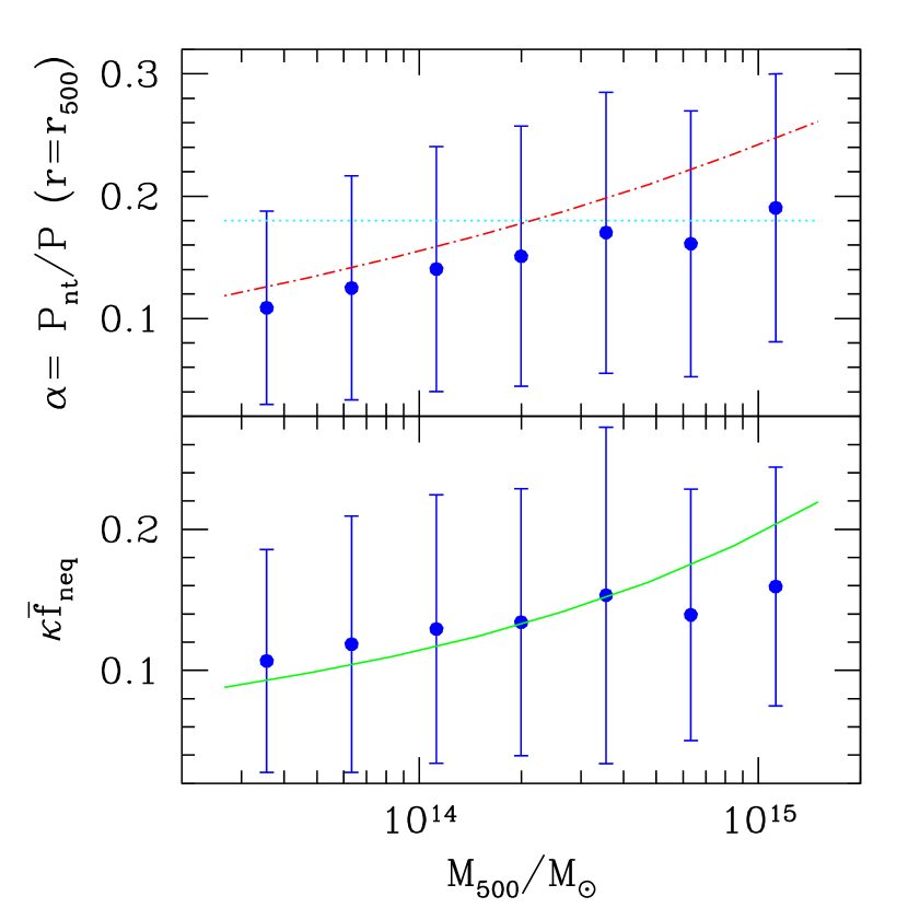
Figure 3: Top: $\alpha=P_{nth}/P$ at $r=r_{500}$, as a function of mass, for halos with redshift $<0.2$. Points with error bars show the mean and standard deviation in logarithmic mass bins. The dotted line is the SNBL value at $z=0$, $\alpha_{0}=0.18\pm 0.06$. The dot-dashed line includes mass dependence as in Battaglia et al. (2011a). Bottom: $\kappa\bar{f}_{neq}$ of the halos. The line is proportional to the peak height $1/\sigma(M)$.

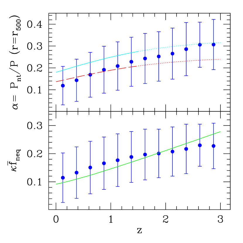
Figure 4: Top: $\alpha$ as a function of redshift, for halos in the range $4\times 10^{13}<M/M_{\odot}<8\times 10^{13}$. Points with error bars show the mean and standard deviation in redshift bins. The upper line uses the SNBL value, $\alpha_{0}=0.18\pm 0.06$; the lower line adjusts this by the mass-dependent term of Battaglia et al. (2011a). Note that these latter two fits are based on $z<1.5$ clusters, and the lines are extrapolated beyond this. Bottom: $\kappa\bar{f}_{neq}$ of the halos. The line is proportional to the peak height $1/\sigma(M)$.

The variation of $\alpha$ with mass at low $z$ (using all halos in the light cone with $z<0.2$) is shown in Fig. 3. At higher masses, the mean is close to the SNBL value of 0.18, but there is a weak mass dependence in the same sense as seen by Battaglia et al. (2011a). However, the mean $\alpha$ scales roughly as $M_{500}^{0.15}$, a slightly shallower scaling than in Eqn. 9. The increase is due primarily to an increase in $\bar{f}_{neq}$ with mass, which is shown in the lower panel of Fig. 4. More massive halos, being rarer, will likely have collapsed more recently and thus be more out of dynamical equilibrium. We can quantify this expectation by considering the peak amplitude $1/\sigma(M)$, where $\sigma(M)$ is the rms density fluctuation on scales corresponding the the spherical tophat collapse of halo of mass $M$. The formation rate of halos at a given mass and redshift will depend on this parameter (e.g. Sheth & Tormen, 1999), as halos with higher peak amplitudes will be more extreme fluctuations. The solid line in the lower panel of Fig. 4 is directly proportional to the peak amplitude, $\kappa\bar{f}_{neq}=0.092/\sigma(M)$. This tracks the mean behavior of the DM halos well, except at the lowest $\sigma$ (highest $M$). The other factor determining $\alpha$, the change in $f^{\prime}_{pol}$ with mass, is less important. This change arises because of the changing concentration of the underlying DM halos. $f^{\prime}_{pol}$ increases with concentration, i.e. with decreasing mass; but as concentration is quite weakly dependent upon $M$, the change is slight (less than 20%).

The variation of $\alpha$ with redshift is shown in the top panel of Fig. 4. The halos shown are restricted to a small mass range so that the evolution shown is unaffected by the change in the mass function with redshift. At higher $z$, clusters are typically dynamically younger and less relaxed, hence $\alpha$ is larger. The increase in $\alpha$ with redshift is slightly more pronounced than that found by SNBL and Battaglia et al. (2011a); the mean scales as $(1+z)^{0.76}$ out to $z=3$. Again the main driver of this evolution is the variation of $\bar{f}_{neq}$, shown in the lower panel. Assuming $\bar{f}_{neq}$ is proportional to peak height reproduces the trend seen out to $z\approx 1.5$, but again as $\sigma$ becomes small (i.e. higher $z$) this leads to an overestimate. Also, once again the variation of $f^{\prime}_{pol}$ is smaller, at about 20% over the whole redshift range shown.

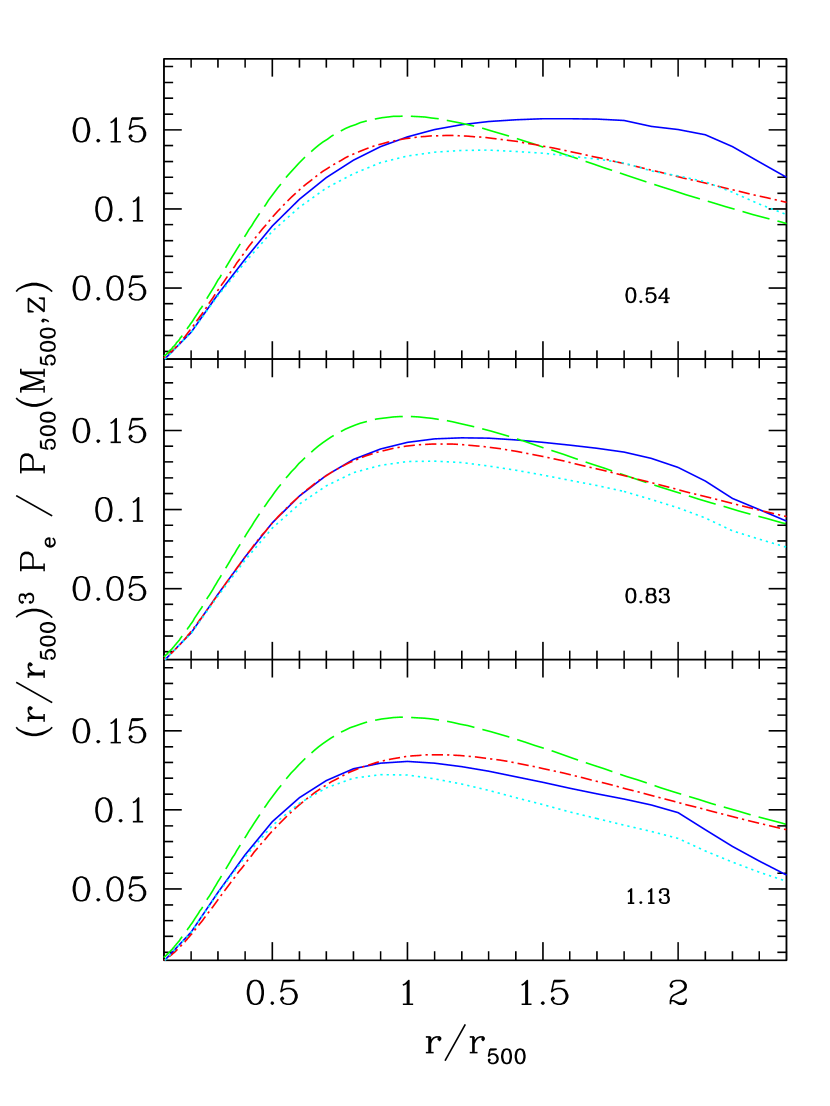
Figure 5: Electron pressure profiles at different redshift. Solid lines: the mean adopted model profile, for selected halos in the mass range $3\times 10^{13}<M_{500}/M_{\odot}<9\times 10^{13}$ and in redshift bins $0.4<z<0.7$, $0.7<z<1.0$, and $1.0<z<1.3$ (panels are labeled with mean redshift). Dashed lines: the low-redshift profile of Arnaud et al. (2010), assuming self-similar scaling to higher $z$. Dot-dashed lines: the mean simulated profile of Battaglia et al. (2011b). Dotted lines: mean profile using Eqn. 8 for $\alpha$ (SNBL).

The evolution with redshift of the mean pressure profile is shown in Fig. 5. A lower mass range was chosen so that the mean mass $\approx 5.6\times 10^{13}M_{\odot}$ does not change with $z$. The model profiles are compared to the Arnaud et al. (2010) profile, which assumes a self-similar evolution. Our model deviates from this assumption; the fit of Battaglia et al. (2011b) deviates in the same manner, but not as strongly. The main processes which can cause a break from self-similarity are star formation and feedback; without matching the evolution of these processes it is difficult to compare methods. However, we have already seen that our method does give a stronger scaling of $\alpha$ with redshift (cf. Fig. 4).

3.3 Setting the level of feedback

The level of feedback, parametrized as $\epsilon_{F}M_{*}c^{2}$, needs to be determined. To constrain $\epsilon_{F}$, we fit to X-ray observations in the $kT-E(z)M_{g}$ plane, where $E^{2}(z)=\Omega_{m}(1+z)^{3}+\Omega_{\Lambda}$. The two samples we compare to are the cluster sample of Mantz et al. (2010) and the lower mass sample of Sun et al. (2009). $M_{g}$ is found inside $r_{500}$, and $T$ is the spectroscopic temperature inside the radial range $[0.15-1]r_{500}$. The simulated sample includes all halos in the light cone with $M_{500}>5.5\times 10^{14}M_{\odot}$ and $z<0.45$, 79 in all, plus another 79 chosen from $z<0.1$ to span the range $2\times 10^{13}<M_{500}<1.5\times 10^{14}$.

To find the best fit we minimize $\chi^{2}$, defined as follows. For simulated halo $i$ and observed cluster $j$ (with observational uncertainties $\sigma_{M}$ and $\sigma_{T}$),

$$c_{ij}=\left(\frac{T_{i}-T_{j}}{\sigma_{Tj}}\right)^{2}+\left(\frac{M_{i}-M_{j}}{\sigma_{Mj}}\right)^{2}\;,$$ (14a)

$$c_{i}=\left(\sum\limits_{j}[c_{ij}]^{-1}\right)^{-1}\;,$$ (14b)

$$\chi^{2}=\sum\limits_{i}c_{i}\;.$$ (14c)

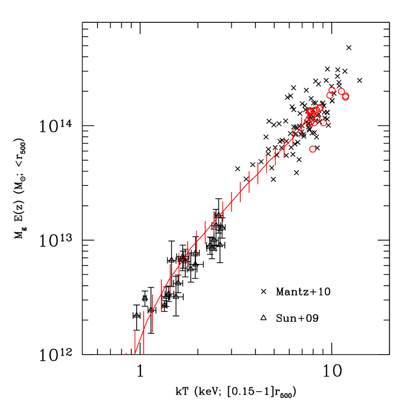
Figure 6: Comparison of the model to X-ray observations by Sun et al. (2009) and Mantz et al. (2010); for the latter, error bars have been omitted for clarity. The red line is the median and vertical bars enclose 68% of the model halos; at the high $T$ end individual halos are shown as circles.

The best fit feedback level when including our model for $\alpha$ is $\epsilon_{F}=8\times 10^{-6}$. If we instead use Eqn. 8, the same value is recovered. The X-ray properties of the model are compared to the observed samples in Fig. 6.

This amount of feedback is larger than that in the Standard model of BOV09, which has no nonthermal pressure. The Standard model value was also chosen to match observed clusters in the $kT-E(z)M_{g}$ plane. Starting with this model, the addition of nonthermal pressure reduces $T$ without making any change to $M_{g}$, so at a given $T$ the value of $M_{g}$ is now too high. Increasing the amount of feedback both reduces $M_{g}$ and increases $T$, bringing the model back into agreement with the observed relation. This amount of feedback is also larger than used by SNBL, but we are also using a lower amount of star formation. As discussed in BOV09, the star formation and feedback parameters are somewhat degenerate, such that increasing the amount of star formation in lower mass clusters would require a lower feedback parameter. Thus a greater amount of feedback is to be expected.

As mentioned in Sec. 2, it is possible to also include relativistic pressure, parametrized as $\delta_{rel}$ times the non-relativistic pressure. However, repeating the above procedure while varying both $\epsilon_{F}$ and $\delta_{rel}$ yields a best fit with $\delta_{rel}=0$, so we do not include it. The main effect from including $\delta_{rel}$ is to increase the total nonthermal pressure in the core. However, there are other, compensating effects we are not including, such as cooling and the presence of a cD galaxy.

4 Implications for the SZ signal

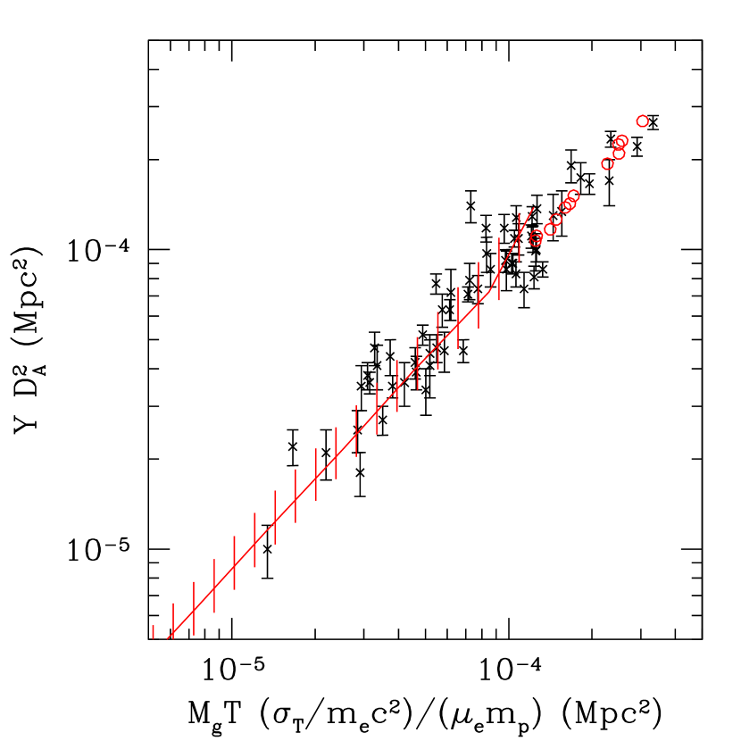
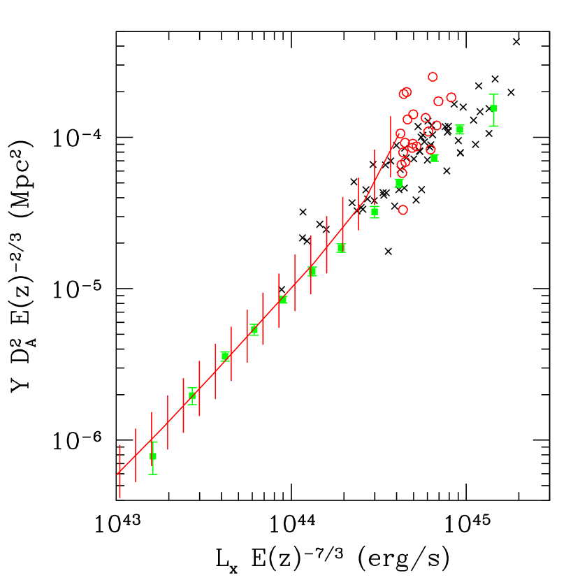
Figure 7: Comparison of the model to X-ray and SZ observations by Planck Collaboration & et al. (2011b, a). Left: points with error bars are from Planck Collaboration & et al. (2011b). The red line is the median and vertical bars enclose 68% of the model halos; at large $Y$ individual halos are shown as circles. $M_{g}$ is measured inside $r_{500}$ and $T$ in the radial range [0.15-0.75]$r_{500}$. All model halos in the light cone with $z<0.5$ are included. Right: SZ signal versus X-ray luminosity in the band [0.1-2.4]keV, measured inside $r_{500}$. Squares with error bars are binned clusters from Planck Collaboration & et al. (2011a); crosses are individual clusters from Planck Collaboration & et al. (2011b) with error bars omitted for clarity.

Having set the parameters of the model by comparison to X-ray observables and simulations, it is now possible to make predictions concerning the SZ signal. We begin by comparing to early results from the Planck satellite. Planck Collaboration & et al. (2011b) combine measurements of $D^{2}_{A}Y=\int P_{th}dV$ inside $r_{500}$ with X-ray data taken by XMM-Newton for 62 $z<0.5$ clusters. $Y$ is expected to scale closely with the X-ray quantity $Y_{X}=CM_{g}T$. Here $C=\sigma_{T}/(m_{e}c^{2}\mu_{e}m_{p})$, where $\sigma_{T}$ is the Thompson cross-section, $m_{e}c^{2}$ is the electron rest mass, and $\mu_{e}m_{p}$ is the mass per electron in a fully ionized plasma. The data from Planck Collaboration & et al. (2011b) is shown in the left-hand panel of Fig. 7; the gas mass $M_{g}$ is measured inside $r_{500}$, and $T$ is measured in the radial range [0.15-0.75]$r_{500}$. For the $f_{nth}$ model clusters we include all halos in the light cone with $z<0.5$. Fitting those with $D^{2}_{A}Y>10^{-5}$Mpc², the slope of the $D^{2}_{A}Y-Y_{X}$ relation is consistent with unity; this agrees with Planck Collaboration & et al. (2011b), but is roughly 2-sigma steeper than the slope found by Rozo et al. (2012). If, following Rozo et al. (2012), we make the pivot point $8\times 10^{-5}$Mpc², then the model gives $\ln(D^{2}_{A}Y/Y_{X})=-0.152\pm 0.002$ with rms scatter $\sigma=0.031$; in other words $(D^{2}_{A}Y/Y_{X}=0.86$, significantly lower than the best fit given by Planck Collaboration & et al. (2011b). On the other hand, it is higher than the analysis of a subsample of the Planck clusters using different X-ray data by Rozo et al. (2012), who find $D^{2}_{A}Y/Y_{X}=0.82\pm 0.024$. These results are insensitive to the redshift range used, but including clusters with $D^{2}_{A}Y$ below $10^{-5}$Mpc² lowers the ratio to $(D^{2}_{A}Y/Y_{X}=0.82$ and increases the scatter to $\sigma=0.037$.

The relation between SZ signal and the X-ray luminosity is shown in the right-hand panel of Fig. 7. The luminosity $L_{X}$ is in the band [0.1-2.4]keV, measured inside $r_{500}$. The same clusters from Planck Collaboration & et al. (2011b) are shown, as well as data for lower-mass clusters from Planck Collaboration & et al. (2011a), who measured $Y$ for roughly 1600 X-ray selected clusters and averaged the results in bins of $L_{X}$. The model reproduces the observed relation well except at the highest $L_{X}$, where the model cores are not dense enough. $Y_{X}$ depends roughly linearly on gas density, and the core was excluded when computing $T$. In contrast, $L_{X}$ depends on the square of density, and thus strongly weights the cluster center. Our model does not include cooling in the cluster core; such cooling would result in higher $L_{X}$ without significantly affecting $Y$ or $Y_{X}$. The slope of the $f_{nth}$ model $L_{X}-Y$ relation (set mostly by the lower mass clusters) is 1.09, in good agreement with Planck Collaboration & et al. (2011a). For this model, the evolution of $Y$ with redshift follows the standard self-similar scaling out to $z=1$.

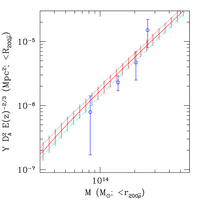
Figure 8: Projected cylindrical SZ decrement for halos hosting LRGs. Circles with error bars are from ACT data, with masses estimated from weak lensing (Hand et al., 2011). The radio-quiet LRG sample is shown; masses are measured inside 200 times the mean density. The solid red line with vertical bars is the median and 68% range of the $f_{nth}$ model clusters. The dotted line is the median for the Standard model of BOV09, and the dashed is for the nonthermal20 model of Trac et al. (2011).

The above comparisons were all measured within of $r_{500}$, whereas the effect of nonthermal pressure is greatest outside this radius. Recently Hand et al. (2011) used ACT data to measure the $Y$ out to a cylindrical radius corresponding to a cluster density of 200 times the mean. This includes the entire contribution along the line of sight, as well as a larger solid angle than subtended by $r_{500}$, and so is more sensitive to the cluster outskirts. The measurement was done by stacking the locations of LRGs, which reside in massive halos, to find the projected SZ signal. This data is shown in Fig. 8. Only the radio-quiet LRG sample is shown, to avoid contamination. The masses of the halos are determined from weak lensing, as the masses determined from bias may be affected by systematics (More, 2011). The model fits the data within the errors.

Fig. 8 also shows the mean relation for the Standard model of BOV09. This model has no nonthermal pressure and a lower amount of feedback, such that inside $r_{500}$ it would closely resemble the $f_{nth}$ model. Because of higher thermal pressure outside this radius, it shows a larger SZ signal. Including $f_{nth}$ has little effect on the slope of the relation, but reduces $Y$ at a given mass by 15% from the Standard model. We also show the nonthermal20 model of Trac et al. (2011); this has constant 20% nonthermal pressure at all radii (note it has a different level of star formation and feedback as well). Thus, while it has a higher thermal pressure at large radii, it will have more nonthermal support in the core, and thus the central density and thermal pressure will be lower. This leads to a smaller value of $Y$ at a given mass. However, the slope of this relation is again little changed.

The reduced SZ signal predicted when $f_{nth}$ is included will alter the predicted angular power spectrum in SZ maps. Computing the $C_{l}$ in the same manner as Trac et al. (2011), the $f_{nth}$ model yields a thermal SZ template 24% lower than the Standard model (at 280 GHz, for $\sigma_{8}=0.8$). Two effects which one might expect could alter the shape of the template, the generally lower $P_{nth}$ in cluster outskirts and the variation in the level of $f_{nth}$ from cluster to cluster, appear not to do so; the peak of the SZ power, at $l\approx 3000$, remains the same. This is in contrast to the nonthermal20 model, which is 45% lower than the Standard model, and has a peak at slightly larger angular scales. The reduction of 24% from the Standard model used in Sehgal et al. (2010) will alleviate somewhat, but not eliminate, the tension with observations (Sehgal et al., 2010; Dunkley et al., 2010; Reichardt et al., 2011).

To summarize, in this paper we have presented a method of including turbulent pressure in a model of the ICM, similar to that of SNBL. The fraction of pressure in turbulent form is allowed to vary from cluster to cluster, depending on the host halo’s dynamical state. The normalization is set by comparing the pressure profiles to X-ray observations and hydrodynamical simulations. The nonthermal pressure fraction measured at $r_{500}$ is typically in the range 10-20%, trending higher with cluster mass and with redshift. This will be useful in creating improved templates for interpreting new data from millimeter and microwave instruments such as the PLANCK satellite. However, a better understanding of the thermodynamic state of the ICM at higher redshifts will be needed to fully exploit this new data.

References

- Agertz et al. (2007) Agertz, O., Moore, B., Stadel, J., Potter, D., & et al. 2007, MNRAS, 380, 963, arXiv:astro-ph/0610051
- Akamatsu et al. (2011) Akamatsu, H., Hoshino, A., Ishisaki, Y., Ohashi, T., Sato, K., Takei, Y., & Ota, N. 2011, PASJ, 63, 1019, 1106.5653
- Andreon (2010) Andreon, S. 2010, MNRAS, 407, 263, 1004.2785
- Arnaud et al. (2010) Arnaud, M., Pratt, G. W., Piffaretti, R., Böhringer, H., Croston, J. H., & Pointecouteau, E. 2010, A&A, 517, A92+, 0910.1234
- Balogh et al. (2011) Balogh, M. L., Mazzotta, P., Bower, R. G., Eke, V., Bourdin, H., Lu, T., & Theuns, T. 2011, MNRAS, 412, 947, 1011.0602
- Battaglia et al. (2011a) Battaglia, N., Bond, J. R., Pfrommer, C., & Sievers, J. L. 2011a, ArXiv e-prints, 1109.3709
- Battaglia et al. (2011b) ——. 2011b, ArXiv e-prints, 1109.3711
- Bautz et al. (2009) Bautz, M. W., Miller, E. D., Sanders, J. S., & et al. 2009, PASJ, 61, 1117, 0906.3515
- Bode et al. (2009) Bode, P., Ostriker, J. P., & Vikhlinin, A. 2009, ApJ, 700, 989, 0905.3748
- Bode et al. (2007) Bode, P., Ostriker, J. P., Weller, J., & Shaw, L. 2007, ApJ, 663, 139, arXiv:astro-ph/0612663
- Bryan (1999) Bryan, G. L. 1999, Comput. Sci. Eng., Vol. 1, No. 2, p. 46 - 53, 1, 46
- Bryan & Norman (1999) Bryan, G. L., & Norman, M. L. 1999, in Structured Adaptive Mesh Refinement Grid Methods, ed. N. P. C. S. B. Baden (IMA Volumes on Structured Adaptive Mesh Refinement Methods, No. 117), 165
- Burns et al. (2010) Burns, J. O., Skillman, S. W., & O’Shea, B. W. 2010, ApJ, 721, 1105, 1004.3553
- Cen (2011) Cen, R. 2011, ApJ, 741, 99, 1104.5046
- Cen et al. (1995) Cen, R., Kang, H., Ostriker, J. P., & Ryu, D. 1995, ApJ, 451, 436, arXiv:astro-ph/9506050
- Cen et al. (2005) Cen, R., Nagamine, K., & Ostriker, J. P. 2005, ApJ, 635, 86, arXiv:astro-ph/0407143
- Cen & Ostriker (1992) Cen, R., & Ostriker, J. P. 1992, ApJ, 399, L113
- Chaudhuri et al. (2012) Chaudhuri, A., Nath, B. B., & Majumdar, S. 2012, ArXiv e-prints, 1203.6535
- Crain et al. (2007) Crain, R. A., Eke, V. R., Frenk, C. S., Jenkins, A., McCarthy, I. G., Navarro, J. F., & Pearce, F. R. 2007, MNRAS, 377, 41, arXiv:astro-ph/0610602
- Das et al. (2011) Das, S., Marriage, T. A., Ade, P. A. R., Aguirre, P., & the ACT Collaboration. 2011, ApJ, 729, 62, 1009.0847
- Di Matteo et al. (2005) Di Matteo, T., Springel, V., & Hernquist, L. 2005, Nature, 433, 604, arXiv:astro-ph/0502199
- Dunkley et al. (2010) Dunkley, J., Hlozek, R., Sievers, J., & the ACT Collaboration. 2010, ArXiv e-prints, 1009.0866
- Eckert et al. (2011a) Eckert, D., Molendi, S., Gastaldello, F., & Rossetti, M. 2011a, A&A, 529, A133+, 1103.2455
- Eckert et al. (2011b) Eckert, D., Vazza, F., Ettori, S., & et al. 2011b, ArXiv e-prints, 1111.0020
- Ettori & Balestra (2009) Ettori, S., & Balestra, I. 2009, A&A, 496, 343, 0811.3556
- Fowler et al. (2010) Fowler, J. W., Acquaviva, V., Ade, P. A. R., & the ACT Collaboration. 2010, ApJ, 722, 1148, 1001.2934
- George et al. (2009) George, M. R., Fabian, A. C., Sanders, J. S., Young, A. J., & Russell, H. R. 2009, MNRAS, 395, 657, 0807.1130
- Giodini et al. (2009) Giodini, S., Pierini, D., Finoguenov, A., Pratt, G. W., & the COSMOS Collaboration. 2009, ApJ, 703, 982, 0904.0448
- Haardt & Madau (1996) Haardt, F., & Madau, P. 1996, ApJ, 461, 20
- Hall et al. (2010) Hall, N. R., Keisler, R., Knox, L., Reichardt, C. L., & the SPT Collaboration. 2010, ApJ, 718, 632, 0912.4315
- Hallman & Jeltema (2011) Hallman, E. J., & Jeltema, T. E. 2011, MNRAS, 418, 2467, 1108.0934
- Hand et al. (2011) Hand, N., Appel, J. W., Battaglia, N., & the ACT Collaboration. 2011, ApJ, 736, 39, 1101.1951
- Hoshino et al. (2010) Hoshino, A., Henry, J. P., Sato, K., & et al. 2010, PASJ, 62, 371, 1001.5133
- Humphrey et al. (2012) Humphrey, P. J., Buote, D. A., Brighenti, F., Flohic, H. M. L. G., Gastaldello, F., & Mathews, W. G. 2012, ApJ, 748, 11, 1106.3322
- Joung et al. (2009) Joung, M. R., Cen, R., & Bryan, G. L. 2009, ApJ, 692, L1, 0805.3150
- Komatsu et al. (2011) Komatsu, E., Smith, K. M., Dunkley, J., & the WMAP Collaboration. 2011, ApJS, 192, 18, 1001.4538
- Lau et al. (2009) Lau, E. T., Kravtsov, A. V., & Nagai, D. 2009, ApJ, 705, 1129, 0903.4895
- Leauthaud et al. (2011a) Leauthaud, A., George, M. R., Behroozi, P. S., & et al. 2011a, ArXiv e-prints, 1109.0010
- Leauthaud et al. (2011b) Leauthaud, A., Tinker, J., Bundy, K., Behroozi, P. S., & et al. 2011b, ArXiv e-prints, 1104.0928
- Lin et al. (2003) Lin, Y.-T., Mohr, J. J., & Stanford, S. A. 2003, ApJ, 591, 749, astro-ph/0304033
- Lin et al. (2012) Lin, Y.-T., Stanford, S. A., Eisenhardt, P. R. M., Vikhlinin, A., Maughan, B. J., & Kravtsov, A. 2012, ApJ, 745, L3, 1112.1705
- Lueker et al. (2010) Lueker, M., Reichardt, C. L., Schaffer, K. K., & the SPT Collaboration. 2010, ApJ, 719, 1045, 0912.4317
- Mahdavi et al. (2008) Mahdavi, A., Hoekstra, H., Babul, A., & Henry, J. P. 2008, MNRAS, 384, 1567, 0710.4132
- Mantz et al. (2010) Mantz, A., Allen, S. W., Ebeling, H., Rapetti, D., & Drlica-Wagner, A. 2010, MNRAS, 406, 1773, 0909.3099
- Marriage et al. (2011) Marriage, T. A., Acquaviva, V., Ade, P. A. R., & the ACT Collaboration. 2011, ApJ, 737, 61, 1010.1065
- McCarthy et al. (2007) McCarthy, I. G. et al. 2007, MNRAS, 376, 497, arXiv:astro-ph/0701335
- Mitchell et al. (2009) Mitchell, N. L., McCarthy, I. G., Bower, R. G., Theuns, T., & Crain, R. A. 2009, MNRAS, 395, 180, 0812.1750
- Morandi et al. (2011) Morandi, A., Limousin, M., Sayers, J., Golwala, S. R., Czakon, N. G., Pierpaoli, E., & Ameglio, S. 2011, ArXiv e-prints, 1111.6189
- More (2011) More, S. 2011, ApJ, 741, 19, 1107.1498
- Nelson et al. (2011) Nelson, K., Rudd, D. H., Shaw, L., & Nagai, D. 2011, ArXiv e-prints, 1112.3659
- O’Shea et al. (2004) O’Shea, B. W., Bryan, G., Bordner, J., Norman, M. L., Abel, T., Harkness, R., & Kritsuk, A. 2004, ArXiv Astrophysics e-prints, astro-ph/0403044
- Ostriker et al. (2005) Ostriker, J. P., Bode, P., & Babul, A. 2005, ApJ, 634, 964, arXiv:astro-ph/0504334
- Paul et al. (2011) Paul, S., Iapichino, L., Miniati, F., Bagchi, J., & Mannheim, K. 2011, ApJ, 726, 17, 1001.1170
- Planck Collaboration & et al. (2011a) Planck Collaboration, & et al. 2011a, A&A, 536, A10, 1101.2043
- Planck Collaboration & et al. (2011b) ——. 2011b, A&A, 536, A11, 1101.2026
- Reichardt et al. (2011) Reichardt, C. L., Shaw, L., Zahn, O., & et al. 2011, ArXiv e-prints, 1111.0932
- Reichert et al. (2011) Reichert, A., Böhringer, H., Fassbender, R., & Mühlegger, M. 2011, A&A, 535, A4, 1109.3708
- Reiprich et al. (2009) Reiprich, T. H. et al. 2009, A&A, 501, 899, 0806.2920
- Rozo et al. (2012) Rozo, E., Vikhlinin, A., & More, S. 2012, ArXiv e-prints, 1202.2150
- Sehgal et al. (2010) Sehgal, N., Bode, P., Das, S., Hernandez-Monteagudo, C., Huffenberger, K., Lin, Y.-T., Ostriker, J. P., & Trac, H. 2010, ApJ, 709, 920, 0908.0540
- Sehgal et al. (2011) Sehgal, N., Trac, H., Acquaviva, V., & the ACT Collaboration. 2011, ApJ, 732, 44, 1010.1025
- Shaw et al. (2010) Shaw, L. D., Nagai, D., Bhattacharya, S., & Lau, E. T. 2010, ApJ, 725, 1452, 1006.1945
- Sheth & Tormen (1999) Sheth, R. K., & Tormen, G. 1999, MNRAS, 308, 119, arXiv:astro-ph/9901122
- Shirokoff et al. (2011) Shirokoff, E., Reichardt, C. L., Shaw, L., & the SPT Collaboration. 2011, ApJ, 736, 61, 1012.4788
- Sijacki et al. (2011) Sijacki, D., Vogelsberger, M., Keres, D., Springel, V., & Hernquist, L. 2011, ArXiv e-prints, 1109.3468
- Simionescu et al. (2011) Simionescu, A. et al. 2011, Science, 331, 1576, 1102.2429
- Sun et al. (2011) Sun, M., Sehgal, N., Voit, G. M., Donahue, M., Jones, C., Forman, W., Vikhlinin, A., & Sarazin, C. 2011, ApJ, 727, L49+, 1012.0312
- Sun et al. (2009) Sun, M., Voit, G. M., Donahue, M., Jones, C., Forman, W., & Vikhlinin, A. 2009, ApJ, 693, 1142, 0805.2320
- Trac et al. (2011) Trac, H., Bode, P., & Ostriker, J. P. 2011, ApJ, 727, 94, 1006.2828
- Urban et al. (2011) Urban, O., Werner, N., Simionescu, A., Allen, S. W., & Böhringer, H. 2011, MNRAS, 414, 2101, 1102.2430
- Vazza et al. (2011a) Vazza, F., Brunetti, G., Gheller, C., Brunino, R., & Brüggen, M. 2011a, A&A, 529, A17+, 1010.5950
- Vazza et al. (2011b) Vazza, F., Dolag, K., Ryu, D., Brunetti, G., Gheller, C., Kang, H., & Pfrommer, C. 2011b, ArXiv e-prints, 1106.2159
- Vieira et al. (2010) Vieira, J. D., Crawford, T. M., Switzer, E. R., & the SPT Collaboration. 2010, ApJ, 719, 763, 0912.2338
- Walker et al. (2012) Walker, S. A., Fabian, A. C., Sanders, J. S., George, M. R., & Tawara, Y. 2012, ArXiv e-prints, 1203.0486
- Young et al. (2011) Young, O. E., Thomas, P. A., Short, C. J., & Pearce, F. 2011, MNRAS, 413, 691, 1007.0887