Radio Emission in the Cosmic Web

Abstract

We explore the possibility of detecting radio emission in the cosmic web by analyzing shock waves in the MareNostrum cosmological simulation. This requires a careful calibration of shock finding algorithms in Smoothed-Particle Hydrodynamics simulations, which we present here. Moreover, we identify the elements of the cosmic web, namely voids, walls, filaments and clusters with the use of the SpineWeb technique, a procedure that classifies the structure in terms of its topology. Thus, we are able to study the Mach number distribution as a function of its environment. We find that the median Mach number, for clusters is $\mathcal{M}_{\mathrm{clusters}}\approx 1.8$, for filaments is $\mathcal{M}_{\mathrm{filaments}}\approx 6.2$, for walls is $\mathcal{M}_{\mathrm{walls}}\approx 7.5$, and for voids is $\mathcal{M}_{\mathrm{voids}}\approx 18$. We then estimate the radio emission in the cosmic web using the formalism derived in Hoeft & Brüggen (2007). We also find that in order to match our simulations with observational data (e.g., NVSS radio relic luminosity function), a fraction of energy dissipated at the shock of $\xi_{\mathrm{e}}=0.0005$ is needed, in contrast with the $\xi_{\mathrm{e}}=0.005$ proposed by Hoeft et al. (2008). We find that 41% of clusters with $M\geq 10^{14}M_{\odot}$ host diffuse radio emission in the form of radio relics. Moreover, we predict that the radio flux from filaments should be $S_{150MHz}\sim 0.12$ $\mu$Jy at a frequency of 150 MHz.

1 Introduction

In the standard theory of formation history, matter evolved from small perturbations in the primordial density field into a complex structure of sheets and filaments with galaxy clusters at the intersections of this filamentary structure. Galaxy surveys, such as the 2dF-GRS (2 degree Field Galaxy Redshift Survey, Colless et al., 2003) and the SDSS (Sloan Digital Sky Survey, Tegmark et al., 2004), have revealed a complex network of filamentary nature, which has become necessary known as the cosmic web (Bond et al., 1996).

In the evolution of the cosmic web, baryons in the diffuse intergalactic medium accelerate towards dark matter halos under the growing influence of gravity and go through shocks that heat them. These cosmological shocks are a ubiquitous consequence of cosmic structure formation. They are tracers of the large-scale structure and contain information about its dynamical history. Gas in walls and filaments follows the gravitational potential towards clusters of galaxies, colliding with the intracluster medium (ICM) at speeds of $\gtrsim 1000$ km s^-1. While cosmological shocks heat the ICM to temperatures of $\sim 10^{7}-10^{8}$ K, filaments are heated to temperatures of $10^{5}-10^{7}$ K, making their detection at present time challenging, since at this temperature there are hardly any emission lines. Therefore, the study of shocks may provide an independent and complementary way to study the Warm-Hot Intergalactic Medium (WHIM), the low density intergalactic medium of the cosmic web that is believed to host the majority of the fraction of the baryon density.

Some cosmological shocks are associated with diffuse radio emission caused by electrons accelerated to relativistic velocities by Fermi acceleration (Enßlin et al., 1998; Roettiger et al., 1999; Miniati et al., 2001). This diffuse radio emission, without galaxy counterpart, is usually divided into two classes, namely radio halos and radio relics. Radio halos are unpolarized and have diffuse morphologies that are similar to those of the thermal X-ray emission of the cluster gas (Giovannini et al., 2006). They are usually found in the center of clusters with significant substructure (see e.g., Cassano et al., 2010).

Radio relics, on the other hand, are typically located near the periphery of the cluster. They have been observed in several merging galaxy clusters. They often exhibit sharp emission edges and many of them show strong radio polarization. Once accelerated, the electrons are short-lived because of the inverse Compton scattering and synchrotron energy losses, and their spectrum rapidly steepens from the shock edge (Giacintucci et al., 2008; van Weeren et al., 2009) The synchrotron nature of this radio emission indicates the presence of cluster magnetic fields of the order of $\sim 0.1-1$ $\mu$G (Feretti & Giovannini, 2008).

Cosmic shocks in large-scale structures have been investigated in a number of semi-analytical (Gabici & Blasi, 2003; Berrington & Dermer, 2003; Keshet et al., 2003; Meli & Biermann, 2006) and numerical work (Miniati et al., 2000, 2001; Miniati, 2002; Ryu et al., 2003; Kang et al., 2005; Pfrommer et al., 2006, 2007, 2008; Jubelgas et al., 2008; Hoeft et al., 2008; Skillman et al., 2008; Battaglia et al., 2009; Vazza et al., 2009; Skillman et al., 2010). Some studies have focused on the non-thermal emission from galaxy clusters by modeling discretized cosmic ray (CR) energy spectra. A series of papers explored the dynamical impact of cosmic ray (CR) protons on hydrodynamics in cosmological SPH simulations (Pfrommer et al., 2006; Enßlin et al., 2007; Jubelgas et al., 2008). Observationally, detecting shocks waves in large-scale structures is still challenging, since they usually develop in the external regions of galaxy clusters, where the X-ray emission is faint. However, a few merger shocks have been detected in nearby X-ray bright galaxy clusters (Markevitch et al., 2005; Markevitch, 2006; Solovyeva et al., 2008) and may be possible associated with a single or double radio relics discovered in a number of galaxy clusters (e.g., Röttgering et al., 1997; Markevitch et al., 2005; Bagchi et al., 2006; Bonafede et al., 2009; Giacintucci et al., 2008).

In numerical studies, Miniati et al. (2000) studied the quantitative properties of large-scale shocks produced by gas during the formation of cosmic structures by means of hydrodynamical simulations. They showed that shocks form abundantly in the course of structure formation and their topology is very complex and highly connected. They also stated that considering the large size and long lifetime of shocks, they are potentially interesting sites for cosmic-ray acceleration. Ryu et al. (2003) (see also Kang et al. 2005) found that shocks form around sheets, filaments and knots of mass distribution when the gas in void regions accretes onto them.

Pfrommer et al. (2006) studied the properties of structure formation shock waves in cosmological SPH simulations, allowing them to study their role in the thermalization of the plasma as well as for the acceleration of relativistic CRs through diffusive shock acceleration. They find that most of the energy is dissipated in weak internal shocks, with Mach number $\mathcal{M}\sim 2$. On the other hand, collapsed cosmological structures are surrounded by external shocks with much higher Mach numbers ($\mathcal{M}\sim 100$), but they play only a minor role in the energy balance of thermalization. Skillman et al. (2008) computed the production of CRs in a cosmological simulation volume, finding that CRs are dynamically important in galaxy clusters. They also found that shocks with low Mach number typically trace mergers and complex flows, while those with mild and high Mach number ($\mathcal{M}>5$) generally follow accretion onto filaments. In a similar study, Vazza et al. (2009) analyzed the properties of large-scale shocks. They find that the bulk of the energy in galaxy clusters is dissipated at weak shocks, with Mach numbers $\mathcal{M}\approx 1.5$, although slightly stronger shocks are found in the external regions of merging clusters.

Pfrommer et al. (2008) used GADGET simulations of a sample of galaxy clusters, implementing a formalism for CR physics on top of radiative hydrodynamics. They modeled relativistic electrons that are accelerated at cosmic formation shocks and produced in hadronic interactions of CRs with protons of the ICM. They found that the radio emission in clusters is dominated by secondary electrons. Only at the location of strong shocks the contribution of primary electrons may dominate. Later, Battaglia et al. (2009) studied the radio emission for a sample of 10 galaxy clusters extracted from zoomed cosmological simulations. They determined the radio luminosity, spectral index and Faraday rotation measure for regions of the relics and concluded that upcoming radio telescopes, such as LOFAR, MWA, LWA and SKA will discover a substantially larger sample of radio relics. SKA should probe the macroscopic parameters of plasma physics in clusters.

Hoeft et al. (2008) investigated the diffuse radio emission from clusters in cosmological SPH simulations. They found that the maximum diffuse radio emission in clusters depends strongly on their X-ray temperature. They also found that the so-called accretion shocks cause only very little radio emission. They conclude that a moderate efficiency of shock acceleration, namely $\xi_{\mathrm{e}}=0.005$, together with moderate magnetic field, namely 0.07-0.8 $\mu$G, in the region of radio relic are sufficient to reproduce the number density and luminosity of radio relics. Skillman et al. (2010), using AMR simulations, also studied radio emission in galaxy clusters. They investigated scaling relations between cluster parameters such as synchrotron power, mass and X-ray luminosity.

In this paper we follow the approach of Hoeft et al. (2008) but, instead of focusing on galaxy clusters, we investigate whether it is possible to detect radio emission in the entire cosmic web. Due to the low temperature of the accreting gas, the Mach number of external shocks - filaments - is high, extending up to $\mathcal{M}\sim 100$ or higher (Ryu et al., 2003). Therefore, the total radio power generated by infall along filaments will be significantly weaker than infall into a cluster. We will try to determine this total radio power. To this end, we use the approach for detecting and identifying shock fronts and their characteristic Mach number developed by Hoeft et al. (2008). This shock finder is applied to a large $N$-body/SPH simulation. For computing the radio emission, we follow the model elaborated in Hoeft & Brüggen (2007). They assumed that electrons are accelerated by diffuse shock acceleration and cool subsequently by synchrotron and inverse Compton losses. Consequently, the radio emission can be expressed as a function of downstream plasma properties, Mach number and surface area of the shock front. In order to correctly assign a surface area to the SPH particles, we calibrate the radio emission using shock tubes experiments. Of primary importance is the proper identification of the different structures that reside in the cosmic web. To this end, we apply the SpineWeb technique (Aragón-Calvo et al. 2010a, see also Aragón-Calvo et al. 2010c) to the entire simulation. The SpineWeb procedure correctly identifies voids, walls, filaments and clusters present in the cosmic web. It is a powerful method that deals with the topology of the underlying density field of the cosmic web. This allows us to study shock properties and radio emission in the different structures that constitutes the cosmic web. This goes beyond the traditionally internal versus external shock classification suggested by Ryu et al. (2003) and the method of characterizing shocks by their pre-shock overdensity and temperature proposed by Skillman et al. (2008). Applying the radio emission model to the simulation leads to radio-loud shock fronts which we are able to locate within the cosmic web.

This paper is organized as follows. In Section 2 we summarize the characteristics of the $N$-body/SPH simulation. Section 3 describes the Spineweb method. In Section 4 we give a brief description of the physics involving non-radiative shocks and depict how we find shocks in SPH simulations. In order to calibrate the radio emission model, we use shock tube tests which are described in Section 6. The radio emission model is sensitive to the shock surface area. Using the results of the shock tubes, in Section 6.1 we described the method used in order to precisely determine the area of the shock front. In Section 7 we present our results for the shock fronts and radio emission in the MareNostrum Universe. In Section 8 we summarize our findings.

2 The Computer Simulation

In order to study cosmological shock waves in the large-scale structure of the Universe, we use the MareNostrum Universe simulation (Gottlöber & Yepes, 2007), one of the largest cosmological simulations available. It assumes a standard flat $\Lambda$CDM Universe with cosmological parameters $\Omega_{m,0}=0.3$, $\Omega_{b,0}=0.045$, $\Omega_{\Lambda,0}=0.7$ and $h=0.7$, where the Hubble parameter is given by $H_{0}=100h$ km s^-1Mpc^-1. The normalization of the power spectrum is $\sigma_{8}=0.9$. The simulation box has a side length of 500$h^{-1}$Mpc and contains 1024³ gas and 1024³ dark matter particles, with masses of $m_{\mathrm{gas}}=1.45\times 10^{9}h^{-1}$M_⊙ and $m_{\mathrm{dm}}=8.24\times 10^{9}h^{-1}$M_⊙. The initial conditions are followed from a redshift of $z=40$ until the present time ($z=0$) using the massively parallel tree $N$-Body/smoothed particle hydrodynamics (SPH) code GADGET-2 (Springel, 2005). The results presented here are at present time ($z=0$). Radiative processes or star formation are not included in the simulation. The Plummer-equivalent softening was set at $\epsilon_{Pl}=15$ $h^{-1}$kpc in comoving units, and the SPH smoothing length was set to the distance to the 40th nearest neighbor of each SPH particle. Smoothing scales are not allowed to be smaller than the gravitational softening of the gas particles.

To extract the groups and galaxy clusters present in the simulation, we use HOP (Eisenstein & Hut, 1998). HOP assigns a density to every particle by smoothing the density field with a spline cubic kernel using the $n$ nearest neighbors of a given particle. Particles are then linked by associating each particle to the densest particle from the list of its closest neighbor. This process is repeated until it reaches a particle that is its own highest density neighbor. All particles linked to a local density maximum are identified as a group. At this stage, no distinction between a high-density region and its surrounding has been make. To identify halos above a certain density threshold, a regrouping merging procedure is performed. The code first includes only particles that are above some density threshold. Then, it merges all groups for which the boundary density between them exceeds a certain density value. Finally, all groups identified must have one particle that exceeds a density peak to be accepted as an independent group. We associate this density peak with the virial density needed for a spherical region to be in virial equilibrium, $\Delta_{\mathrm{vir}}$. The value of $\Delta_{\mathrm{vir}}$ is obtained from the solution to the collapse of a spherical top-hat perturbation under the assumption that the object has just virialized. For the cosmology described here, at present time its value is $\Delta_{\mathrm{vir}}\approx 337$.

In using HOP, we use the dark matter particles of the MareNostrum simulation. Once we identified the virialized halos of the sample, we take the position of the densest dark matter particle as a first estimate of the center of mass. Subsequently, we add the gas particles, grow a sphere around the center of mass and begin iterating, shrinking the sphere around the (new) center of mass until we reach a minimum of 50 particles. This ensures a correct identification of the center of mass taking into account gas and dark matter particles. Once we have the final center of mass, we grow a sphere around it that encloses a value of $\Delta_{\mathrm{vir}}\approx 337$. Given that we want to study radio emission in the cosmic web, the nodes of the filaments will be consider as galaxy clusters with masses $M>10^{14}h^{-1}$M_☉. We find that the MareNostrum Universe contains 3865 clusters of galaxies, the most massive with a mass of $M=2.5\times 10^{15}h^{-1}$M_☉ and virial radius $R_{\mathrm{vir}}=2.75h^{-1}$Mpc.

3 The SpineWeb procedure

The characterization of the Large-Scale Structure was done using the SpineWeb method (for a thorough explanation see Aragón-Calvo et al. 2010a, see also Aragón-Calvo et al. 2010c). This method classifies the Cosmic Web into four basic morphological and dynamical components: voids, walls, filaments and clusters. The SpineWeb method is based on the Watershed transform (Beucher & Lantuejoul, 1979) and its cosmological implementation: the Watershed Void Finder (WVF) (Platen et al., 2007). The idea behind the WVF is to segment the density field into individual basins by ”flooding” it (in analogy to a landscape). The SpineWeb method takes this analogy and goes one step further by directly relating the topology of the density field and the boundaries between basins by observing the simple relation between number of adjacent basins and topology: walls correspond to the boundary between two voids. Filaments+clusters are found at the intersection of three or more voids, which translates to the intersection of three or more walls:

$$\mathcal{N}_{\textrm{\tiny{voids}}}\qquad\left\{\begin{array}[]{rrl}\quad=\;\;\;1,&\mathrm{void}\\ \quad=\;\;\;2,&\mathrm{wall}\\ \quad\geq\;\;\;3,&\mathrm{spine}\\ &\mathrm{(filament+clusters)}\\ \end{array}\right.$$ (1)

The resulting morphological characterization is parameter-free. The analysis presented here is also based on the most recent implementation of the SpineWeb method which extends the original formalism on a multiscale hierarchical fashion making it also scale-independent.

In practice we start our analysis by generating a low resolution version of the original simulation using the averaging procedure described in Klypin et al. (2001). The lower particle resolution was chosen to correspond to a inter-particle separation of approx. 3$h^{-1}$Mpc at the initial conditions. With this “linear-regime” filtering we avoid small-scale substructure at the present time while keeping the characteristic large-scale anisotropy of the cosmic web. From the particle distribution we compute the density field using the DTFE method (Schaap & van de Weygaert, 2000; Schaap, 2007; van de Weygaert & Schaap, 2009). The field is sampled at 27 different points inside each voxel and its mean is used to estimate the density for that particular voxel. From the density field we compute the watershed transform and identify the boundaries of the basins (i.e. the watershed transform itself). Finally for each voxel in the watershed transform we apply the criteria outlined in Eqn. 1. The complete procedure takes a few minutes on a regular workstation.

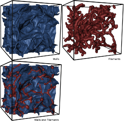
Figure 1: An example of how the SpineWeb procedure divides the cosmic web. Shown are surfaces enclosing voxels which are identified as belonging to walls (blue, top left frame) and filaments (red, top right frame) within a cubic region of 50$h^{-1}$Mpc. The bottom frame shows the same region with both components connected and intertwined.

The SpineWeb method provides a complete framework for the characterization of the cosmic web into its basic morphological constituents: voids, walls, filaments and clusters. It has no free parameters and being fundamentally a topological measure it is highly robust against noise in the density field. Fig. 1 shows an example of how the SpineWeb correctly identifies the different elements of the cosmic web. Shown is a full 3D network of filaments (red) and walls (blue). It is clearly visible the three-dimensional nature of the filament-wall network. Filaments define an interconnected web and walls fill the spaces in between the filaments forming a closed ”watertight” network of voids.

4 Hydrodynamical Shocks and Shock Finder

In the formation of structures in the Universe, the bulk velocity of the gas flow often exceeds the local sound speed. As a result, the shock surface separates two regions: the upstream regime or pre-shock regime, and the downstream regime or post-shock regime. The plasma in the upstream regime moves with a velocity $v_{\mathrm{u}}$ towards the shock front, while the downstream plasma departs with velocity $v_{\mathrm{d}}$. Most of the incident kinetic energy flux is converted into thermal energy. As the plasma passes through the shock front, mass, momentum and energy fluxes are conserved, which is expressed in the Rankine-Hugoniot relations:

$$\rho_{\mathrm{u}}v_{\mathrm{u}}\, = \,\rho_{\mathrm{d}}v_{\mathrm{d}}\,,$$

$$P_{\mathrm{u}}+\rho_{\mathrm{u}}v_{\mathrm{u}}^{2}\, = \,P_{\mathrm{d}}+\rho_{\mathrm{d}}v_{\mathrm{d}}^{2}\,,$$

$$\frac{v_{\mathrm{u}}^{2}}{2}+u_{\mathrm{u}}+\frac{P_{\mathrm{u}}}{\rho_{\mathrm{u}}}\, = \,\frac{v_{\mathrm{d}}^{2}}{2}+u_{\mathrm{d}}+\frac{P_{\mathrm{d}}}{\rho_{\mathrm{d}}}\,,$$ (2)

where $\rho$ denotes the mass density, $P$ is the pressure and $u$ is the specific internal energy, and the velocities are measured in the rest-frame of the shock surface. The strength of a shock is given by the Mach numbers $\mathcal{M}$,

$$\mathcal{M}\,=\,\frac{v_{\mathrm{u}}}{c_{\mathrm{u}}}\,,$$ (3)

where $c_{s}$ denotes the upstream sound speed which depends on the the specific internal energy by $c_{\mathrm{u}}=\sqrt{\gamma(\gamma-1)u_{\mathrm{u}}}$. Combining Eqns. 2 and 3, and assuming that the plasma obeys the polytropic relation, we can write for the Mach number

$$\mathcal{M}^{2}\,=\,\frac{r}{\gamma}\frac{qr^{\gamma}-1}{r-1}\,,$$ (4)

where $r$ and $q$ are the compression and entropy ratios. The difference between downstream and upstream velocity can be written as

$$v_{\mathrm{d}}-v_{\mathrm{u}}\,=\,\mathcal{M}\frac{r-1}{r}u_{\mathrm{u}}\,.$$ (5)

The Mach number estimator, which will be explained in the next section, computes the entropy ratio and the ratio $(v_{\mathrm{d}}-v_{\mathrm{u}})/u_{\mathrm{d}}$ for each SPH particle in the simulation. In order to obtain the Mach number, we tabulate the relations between $q$, $r$, $\mathcal{M}$ and $\mathcal{M}(r-1)/r$, allowing us to simple read the Mach number from a table.

4.1 Shock finder and Mach number estimate

In order to calculate the radio emission present in the MareNostrum simulation, the first step is to identify shock fronts, and from this, derive the Mach number, downstream (postshock) temperature and electron density. The method we employ is the one proposed and used by Hoeft et al. (2008). For a detailed description of the method, we refer to the mentioned paper. Here, we will give the basic details.

The first step consists of computing the entropy gradient, $\nabla S$, for each SPH particle. The entropy gradient gives the direction of the shock normal pointing into the downstream direction. We define an associated upstream and downstream position,

$$\mathbf{x_{li}}\,=\,\mathbf{x_{i}}+f_{h}h_{i}\mathbf{n}^{1}_{i}\,,$$ (6)

where $l=u,d$ denotes upstream or downstream, with the downstream position in the opposite direction, $\mathbf{x}_{i}$ is the position of the SPH particle $i$, $h_{i}$ is the smoothing length of particle $i$ and $\mathbf{n}^{1}_{i}$ denotes the shock normal, $\mathbf{n}^{1}_{i}=-\nabla S/|\nabla S|$.

The upstream and downstream velocity are computed, together with the internal energy and density, using the usual SPH scheme. The upstream velocity is given by $v_{ui}+v_{sh}=\mathbf{v}(\mathbf{x}_{ui})\cdot\mathbf{n}^{1}_{i}$, and the same for the downstream velocity, but using the downstream position. $v_{sh}$ is the velocity of the shock front in the rest-frame of the simulation. It is important to notice that the velocity field can also show perpendicular components. We compute these components in a similar way to the upstream and downstream velocities, $v_{i}^{k\pm}=\mathbf{v}(\mathbf{x}_{i}\pm f_{h}h_{i}\mathbf{n}^{k}_{i})\cdot\mathbf{n}^{k}_{i}$, where the three vectors $\mathbf{n}^{1}$, $\mathbf{n}^{2}$ and $\mathbf{n}^{3}$ form an orthonormal base.

Once this is done, for those particles that belong to a shock front we demand that the velocity has to be divergent in the direction of the shock normal, i.e., $(v_{\mathrm{d}}-v_{\mathrm{u}})>0$. Also, the velocity difference in the directions perpendicular to the shock normal have to be smaller than that parallel to the shock, i.e., $|v_{k}^{+}-v_{k}^{-}|<(v_{\mathrm{d}}-v_{\mathrm{u}})/2$.

Finally, to compute the Mach number, there are two options: it is possible to use the entropy ratio $q=S_{d}\S_{u}$ ($S$ is the entropy) or use the ratio $(v_{\mathrm{d}}-v_{\mathrm{u}})/c_{\mathrm{u}}$, where $c_{\mathrm{u}}$ is the sound speed in the upstream region (see Section 4). In order to have a conservative estimate for the Mach number, the smaller value of these two options is used.

5 Radio Emission Model

In this section, we will briefly describe the radio emission model. For a complete description, we refer to Hoeft & Brüggen (2007) and Hoeft et al. (2008).

The first assumption of the model is that radio emission is produced by electrons accelerated to ultra-relativistic speeds required for synchrotron and inverse Compton radiation. These electrons are accelerated to a power-law distribution that is related to the Mach number from diffusive shock acceleration theory. As for the magnetic field in the downstream region, it is assumed that, on average, simply obeys flux conservation to follow:

$$\frac{B_{\mathrm{d}}}{B_{\mathrm{ref}}}\,=\,\left(\frac{n_{\mathrm{d}}}{10^{-4}\textrm{cm}^{-3}}\right)^{2/3}\,,$$ (7)

where $B_{\mathrm{ref}}$ is $0.1\mu G$ and $n_{d}$ is the number density in the downstream region. This is a simple assumption since a detailed model for the generation and evolution of magnetic fields is complex and beyond the scope of this paper (see, e.g., Bonafede et al. 2010 for a recent study on magnetic fields in the Coma cluster).

There are several indications that the magnetic field intensity decreases going from the center to the periphery of a cluster. The exact power with which it varies with density is unclear, however. Some simulations suggest a higher power than that given by flux conservation which is attributed to the work of a fluctuation dynamo (see e.g. Dolag et al. (2008) and Brüggen et al. (2005)). Faraday rotation measurements in the Coma cluster Bonafede et al. (2010) give a best fit for $B\propto n^{0.5}$. Such a power would decrease the luminosity of cluster shocks by about 20%. Outside of clusters there are even fewer observational constraints. Recent constraints from TeV $\gamma$-ray sources have placed lower limits on extragalactic magnetic fields (EGMFs). The charged particles from pair cascades are deflected by EGMFs, thereby reducing the observed point-like flux. Dolag et al. (2011) have calculated the fluence of 1ES 0229+200 as seen by Fermi-LAT for different EGMF. The non-observation of 1ES 0229+200 by Fermi-LAT suggests that the EGMF fills at least 60% of space with fields stronger than $10^{-15}$ G assuming that the source is stable for at least $10^{4}$ yr. The fields outside clusters, however, will have a negligible effect on the radio luminosity function since the by far the largest part of the radio luminosity originates from shocks in or near clusters.

The radio emissivity, $P(e,\nu_{\mathrm{obs}})$, which depends on three quantities: i) the energy of the electron energy ($e$), ii) the observing frequency ($\nu_{\mathrm{obs}}$), and iii) the magnetic field strength ($B$), is then given by:

$$\frac{\mathrm{d}P(\nu_{\mathrm{obs}})}{\mathrm{d}\nu}\,=\,6.4\times 10^{34}\mathrm{erg}\,\textrm{s${}^{-1}$}\textrm{Hz${}^{-1}$}\,\frac{A}{\textrm{Mpc${}^{2}$}}\frac{n_{e}}{10^{-4}}\textrm{cm${}^{-3}$}$$

$$\times\frac{\xi_{\mathrm{e}}}{0.05}\left(\frac{\nu_{\mathrm{obs}}}{1.4\mathrm{GHz}}\right)^{-s/2}\times\left(\frac{T_{\mathrm{d}}}{7\mathrm{keV}}\right)^{3/2}$$

$$\times\frac{(B/\mu G)^{1+s/2}}{(B_{\mathrm{CMB}}/\mu G)^{2}+(B/\mu G)^{2}}\Psi(\mathcal{M},T_{\mathrm{d}})\,,$$ (8)

where $n_{e}$ is the electron density, $\xi_{\mathrm{e}}$ is the fraction of energy dissipated by the electron at the shock front and $s$ is the compression ratio at the shock front. The radiation spectral index is related to the electron spectral index by $\alpha=(s-1)/2$. $B_{\mathrm{CMB}}$ has a value of $3.24=\mu G(1+z)^{2}$. This magnetic field is defined as the magnetic field corresponding to the energy density of the CMB.

As stated before, in order to calculate the radio emission, we need the Mach number, $\mathcal{M}$, the downstream temperature, $T_{\mathrm{d}}$, the electron density, $n_{e}$, the magnetic field, $B$, and the shock surface area, $A$. The shock finder described in Sect. 4.1, besides locating shock discontinuities in a SPH simulation, also provides estimates for the Mach number and for the shock normal. This normal vector gives a position which is sufficiently downstream to determine $T_{\mathrm{d}}$ and $n_{e}$. As for the shock surface area $A$, each particle represents an area of the shock, since a shock front is comprised of particle in a SPH simulation. The shock discontinuity is smoothed by the size of the SPH kernel, $h_{\mathrm{SPH}}$, which contains $N_{\mathrm{SPH}}$ particles, with a corresponding volume of $h^{3}_{\mathrm{SPH}}$. Therefore, one particle belonging to the shock front represents a shock area of

$$A\,=\,f_{\mathrm{\small{A}}}\frac{h_{\mathrm{\small{SPH}}}^{2}}{N_{\mathrm{SPH}}}\,,$$ (9)

where $f_{\mathrm{A}}$ is a normalization constant which was set to be $6.5$ by Hoeft et al. (2008) using shock tube simulations. Here, we will correct this factor also using shock tubes, as it was found that $f_{\mathrm{A}}$ depends strongly on $\mathcal{M}$ for low Mach number shocks (see next section).

$\mathcal{M}$	$P_{\mathrm{1}}$	$\mathcal{M}_{fit}$	$\sigma(\log{\mathcal{M}})$
1.4	992285.25	1.38	0.003
1.5	789384.98	1.48	0.003
2	348961.73	1.97	0.003
3	133227.50	2.92	0.007
6	30602.35	5.25	0.020
10	10825.70	8.61	0.023
30	1192.46	25.41	0.031
60	297.87	50.47	0.034
100	107.22	84.14	0.035
300	11.91	246.04	0.042
500	4.29	407.38	0.045
700	2.19	566.24	0.046
1000	1.07	803.53	0.050
1300	0.63	1042.32	0.051
1500	0.48	1199.50	0.051
1800	0.33	1419.06	0.053

Table 1: Shock tube tests parameters. The columns indicate the strength of the shock, i.e., the Mach number $\mathcal{M}$, the pressure in the high density region, the fitted Mach number and the standard deviation, $\sigma$, of the fitted Gaussian.

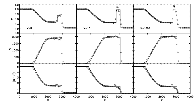
Figure 2: Simulations of the Sod shock tube problem with Mach numbers $\mathcal{M}=3$, $10$ and $1000$. The numerical result of the volume-averaged hydrodynamical quantities within bins with a spacing equal to the inter-particle separation of the high-density medium is shown in open circles while the analytical result is shown as continuous lines. The upper row shows the density $\rho$ of the gas, the middle row shows the velocity $v_{x}$, while the bottom row depicts the pressure of the gas.

6 Calibrating the Radio Emission

An important quantity in Eqn. 8 is the shock surface area, which depends on the normalization factor $f_{\mathrm{A}}$. Hoeft et al. (2008) determined this factor using shock tube tests, finding that it depends on the Mach number of the shock. The origin of this is the following: the Mach number estimator results in a distribution of Mach numbers for the particles in the SPH-broadened shock discontinuity, i.e., in the periphery of the shock front the Mach number is underestimated. For small Mach numbers, $\mathcal{M}\lesssim 5$ the radio emission depends strongly on $\mathcal{M}$, while for large Mach numbers it does not. Therefore, a constant $f_{\mathrm{A}}$ underestimates the radio emission of shocks with $\mathcal{M}\lesssim 5$. Next, we determine the function $f_{\mathrm{A}}(\mathcal{M})$ by calibrating it with shock tube tests.

We run several shock tube tests in order to model a large range of Mach numbers and, therefore, obtaining a proper area function. We construct 16 standard shock tube tests (Sod, 1978) using a 3D-version of the GADGET2 code (Springel, 2005). We consider an ideal gas with $\gamma=5/3$, initially at rest. The left-half space ($x<2000$) is filled with gas at unit density, $\rho_{2}=1$ and pressure $P_{2}=5\times 10^{6}$, while the right half, $x>2000$, is filled with low-density gas, $\rho_{1}=0.25$ and variable low-pressure. The value of this low-pressure gas has been chosen such that the resulting solutions yield the Mach numbers in the range of $\mathcal{M}=1.4-1800$. We set up the initial conditions in three dimensions using an irregular glass-like distribution. In order to test the differences in resolution, we ran the same tests in different resolutions: from $12500$ particles to $800000$ particles. We did not find any significant difference between these resolutions. Hence, the results presented here are done with shock tubes with $100000$ particles. The particles are contained in a periodic box which is longer in the $x$-direction than in the other two dimensions, $y$ and $z$. The parameters of the different shock tube tests are shown in Table 1.

Fig. 2 shows the profile of gas density, velocity and pressure in a shock tube calculation where the gas particles experience a shock of Mach number $\mathcal{M}=10$. The simulation results are presented by circles and the continuous lines give the analytic solution. The shock tube simulations were run with the same SPH parameters (e.g., artificial viscosity) as the MareNostrum Universe in order to compare results. Overall, there is a good agreement between the analytical and the numerical solution, with discontinuities resolved in about two to three SPH smoothing lengths. There is a characteristic pressure blip at the contact discontinuity. The irregularities observed in the density profile may be due to the small number of particles in the SPH kernel, namely $N_{\mathrm{SPH}}=40$.

We calculate the strength of the shock with the Mach number estimator. Although the shock tube was run with $N_{\mathrm{SPH}}=40$, the shock finder was set up with $N_{\mathrm{SPH}}=80$ in order to smooth the fields. To determine the function $f_{\mathrm{A}}(\mathcal{M})$, we calculate the differential shock surface area in logarithmic Mach number bins, $dS/d\log{\mathcal{M}}$, for each of the shock tubes. Fig. 3 shows such distribution for the shock tube calculation with $\mathcal{M}=10$. The surface area was calculate using Eqn. 9 setting $f_{\mathrm{a}}=1$ in order to obtain $f_{\mathrm{a}}(\mathcal{M})$. Visual inspection allow us to draw two observations. Firstly, there is a small shift in the value of the theoretical Mach number and the one estimated by the shock finder meaning the shock finder is underestimating the Mach number. Secondly, there is a “tail” of shock surface areas to the left of the Gaussian-like distribution. This has the following origin: the shock finder identifies low-Mach number shocks in the periphery of the transition region between the upstream and the downstream zone (see Fig. 2) given the nature of SPH, i.e., quantities are calculated over a region determined by $N_{\mathrm{SPH}}$. Hence, the tail has surface area contribution from the upstream and downstream region.

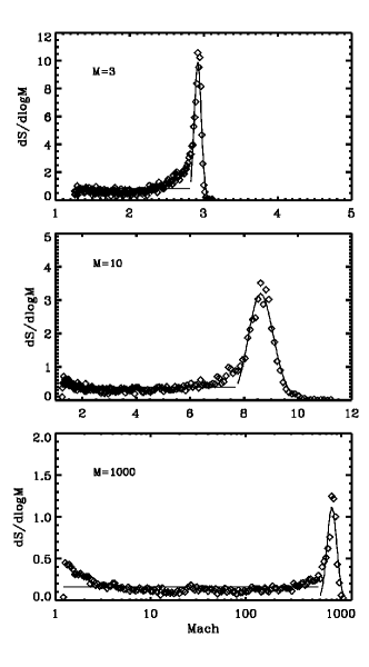
Figure 3: Differential shock surface area as a function of logarithmic Mach number bins for a shock tube calculation with $\mathcal{M}=10$. The differential shock surface area is normalized by the binsize and the cross section of the tube. Solid line represents the bestr fit of the Gaussian-like distribution and the constant surface area to the left of the Gaussian.

We calculate the shock surface area of all shock tube realizations. Every shock tube exhibits a similar $dS/d\log{\mathcal{M}}$ distribution as the one shown in Fig. 3. We fit the distribution with a Gaussian centered on the mean Mach number $\bar{\mathcal{M}}$ (which should be the theoretical Mach number) and a Heaviside function $\mathcal{H}$ multiplied by a constant factor $\mathcal{K}$ which is determined as the mean value of the surfaces areas located approximately $3\sigma$ to the left of the Gaussian mean value, i.e.,

$$f(\log{\mathcal{M}})\,=\,\left\{\begin{array}[]{rrl}\mathcal{K}\cdot\mathcal{H}(\mathcal{X})&\;\;\mathrm{for}&\log{\mathcal{M}}\leq\log{\bar{\mathcal{M}}}-3\sigma\\ e^{-\mathcal{X}^{2}/2\sigma^{2}}&\;\;\mathrm{for}&\log{\mathcal{M}}>\log{\bar{\mathcal{M}}}-3\sigma\end{array}\right.$$ (10)

where $\mathcal{X}=\log{\mathcal{M}}-\log{\bar{\mathcal{M}}}$.

Each shock tube gives us 3 different fitting values: the constant $\mathcal{K}$, the mean of the Gaussian function $\bar{\mathcal{M}}$ and the standard deviation of the Gaussian, $\sigma$. Fig. 4 shows the best fits to the mentioned variables. Although we were able to fit the constant $\mathcal{K}$ in two segments of Mach numbers, we find it is, on average, $\sim 10\%$ of the peak value of the Gaussians. For $\mathcal{M}$ and $\sigma$, we see there is a good correspondence with the theoretical Mach number. We can, therefore, do a linear fit, obtaining functions that will deliver a correct Mach number $\mathcal{M}$ that will be applied to the radio emission model.

6.1 Calculating the Shock Area

To correctly calculate the radio emission, we need to correct the normalization constant $f_{\mathrm{A}}(\mathcal{M})$ (see Eqn. 9).To this end, we find the area within 2$\sigma$ around the mean Mach number of each shock tube, $S_{\mathrm{exp}}$. This area should be similar to the cross section of the tube, $S_{\mathrm{theo}}$. We find a relation between the Mach number and the ratio $S_{\mathrm{theo}}/S_{\mathrm{exp}}$:

$$f_{\mathrm{A}}(\mathcal{M})\,=\,0.54\log{\mathcal{M}}\,+\,5.71\,.$$ (11)

The fitting obtained in the previous section together with Eqn. 11, allows us to correctly estimate the radio emission (Eqn. 8) in the simulation.

Another important quantity we want to determine from the MareNostrum simulation is the shock surface area in a given logarithmic Mach number interval. However, as seen in the previous section, our shock finder algorithm underestimates high Mach numbers and, due to the SPH nature, for high Mach numbers it identifies low shock Mach numbers to particles involved in the shock front. In order to correct this, we will use the results of the previous section and deconvolve them with the measured $dS/d\log{\mathcal{M}}$ distribution, i.e., we will deconvolve the shock surface area distribution calculated from the MareNostrum simulation with a deconvolution kernel obtained by constructing the function of Eqn. 10. We do this by using a deconvolution technique which is explained in Appendix A.

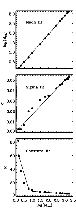
Figure 4: Best fits to the different variables of the Gaussians. Upper panel: linear fit of the measured Mach number. Central panel: linear fit of the $\sigma$ of the Gaussian distribution. Bottom panel: linear fit to the constant $\mathcal{K}$ left to the Gaussians fits.

Fig. 5 shows the measured $dS/\log{\mathcal{M}}$ distribution obtained from the MareNostrum simulation (solid line) and the “real” distribution obtained with the deconvolution technique (filled circles linked by a dotted line), where we have also used the Mach number shift obtained from fitting $\bar{\mathcal{M}}$ from the shock tubes. As expected from the shock tube data, the real distribution has lower Mach numbers, expressed in a smaller shock surface area, while it has more high Mach numbers for $\mathcal{M}\gtrsim 10$.

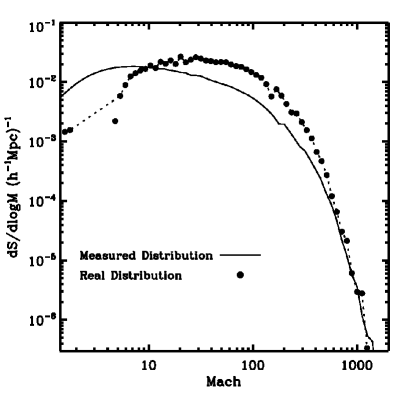
Figure 5: Shock surface area in logarithmic bins as a function of Mach number. Solid line depicts the measured distribution obtained from the MareNostrum simulation. Filled circles shows the “real” distribution, i.e., the distribution obtained by deconvolving the measured distribution with the data from the shock tubes.

The Mach number determination is constructed in a way that it results in a conservative estimate even in more complex situations. We would like to demonstrate this by a colliding shock tube simulation. We have set up a shock tube with three initial zones, with densities and internal energies so that two shocks with Mach number 10 forms later on, see Fig. 6. Our shock finder detects the shock fronts even when the actual shock is not spatially separated from the initial pressure jump. In the shock finder the Mach number is estimated via two methods: firstly it evaluates the velocity field and secondly it uses the entropy jump. In the initial set-up the entropy jump would lead to a Mach number of 10, corresponding to the actual Mach number. However, particles needs to be accelerated to form the corresponding velocity field. Therefore the shock finder underestimates the Mach number in the beginning of the simulation. Later on, when the two shock fronts get close to each other, the shock finder includes particles from the downstream region of the oncoming shock, hence, it does not measure the actual upstream properties anymore. A mach number estimate based on the velocity field would significantly overestimate the Mach number, since the detected velocity divergence would be spuriously high. However, the entropy now causes that the shock finder underestimates the Mach number. Therefore, our shock finder tends to provide only a lower estimate for the Mach number in complex situations, where e.g. several shock fronts overlap.

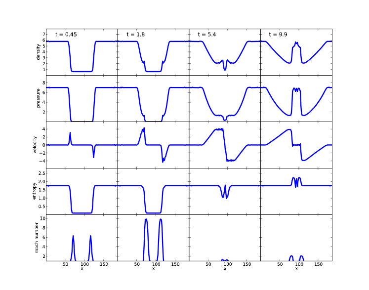
Figure 6: Simulation of two cooling shocks. The initial densities and pressures are chosen in way that two shock fronts each with Mach number 10 forms when the simulation starts.

6.2 Correcting the floor temperature

One last step is to correct for the floor temperature of the MareNostrum simulation. Mach numbers are sensitive to the temperatures of the different environments. Since the simulation was run with a low floor temperature (200 K) and without any UV background, expansion cooling leads to very low temperatures. This can result in unrealistically high Mach numbers. However, the UV background heating leads to a simple power law between the temperature and the density, so the temperature of cold regions (underdense regions) can be scaled by (Hui & Gnedin, 1997)

$$T\;=\;T_{0}(1+\delta)^{\gamma-1}\,,$$ (12)

for regions with $\delta\lesssim 5$, where $\delta$ is the density contrast, and temperature $T_{0}$. We apply this relation to low-density particles. Fig. 7 shows the Mach number distribution with the “old” floor temperature (solid lines) and with the corrected temperatures. Two effects can be seen: i) by correcting the temperature, more particles get assigned a Mach number, and ii) the values of the Mach numbers decreases, i.e., UV background heating plays an important role in cosmological shocks. Nonetheless, if we compare our results to those of Skillman et al. (2008), there still high Mach numbers. In their simulations, they did not find shocks above $\mathcal{M}\approx 200$. This may be due to the fact that the floor temperature was too low, so any scaling to those low temperatures, which, in general, are in underdense regions, will result in a low increment of the temperature. In the case of Skillman et al. (2008), their floor temperature was set at $T=10^{4}$ K, thus assuming the low-density gas to be ionized.

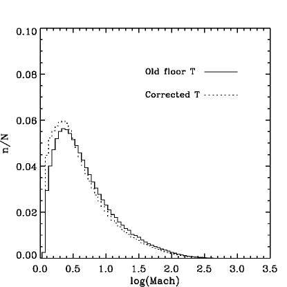
Figure 7: Histogram showing the Mach number distribution when the original MareNostrum floor temperature is used (solid line), and when applying Eqn.  (dotted lines).

The results in the following sections are done using the corrected temperature values.

7 Results

7.1 Shock Frequency in the Cosmic Web

We computed the surface area of identified shocks per logarithmic Mach number interval, $dS(\mathcal{M})/\log{\mathcal{M}}$ as described in Section 6.1. We divide the shock surface area by the volume of the simulation box, as done in Ryu et al. (2003). The inverse of the shock surface area, $1/S$, can be of thought as a mean separation of shocks because it is the simulation volume divided by the total shock surface area. The $dS(\mathcal{M})/\log{\mathcal{M}}$ distribution also indicates the frequency with which shocks happen in the Universe.

Instead of studying and classifying shocks as internal or external as done by Ryu et al. (2003), we use the SpineWeb technique (see Section 3) in order to characterize voids, walls, filaments and clusters by their morphology. Aragón-Calvo et al. (2010b) found that while all morphologies occupy a roughly well-defined range in density, this is not sufficient to differentiate between them given their overlap. Environment defined only in terms of density fails to incorporate the intrinsic dynamics of each morphology. Nevertheless, we also construct the differential shock surface area distribution by using density and temperature cuts in order to compare with Skillman et al. (2008).

Fig. 8 shows the differential shock surface area as a function of logarithmic Mach number bins. The top left panel shows the shock surface area of the different elements of the cosmic web as computed by the SpineWeb procedure. The top right panel shows the latter results after deconvolving them with the method outlined in Appendix A. The bottom left panels shows the distribution divided into several ranges of overdensity values, while the bottom right panel shows the distribution divided in temperature ranges.

We see that there is a large range of shocks of different strengths, with Mach numbers in the range $\mathcal{M}=1.5\sim 1700$. However, it is important to notice that the large Mach numbers may not occur in reality, and even the correction applied to the temperatures in the low-density regions (see Section 6.2 may not be enough to correctly correct the temperatures in the low density regions.

When looking at the top panels, we observe that each element of the cosmic web has a distinctive shock surface area distribution, which follows their characteristic density and temperature distribution and the dynamics between them. After deconvolving the shock surface area distribution obtained from the MareNostrum simulation using the method outlined in Appendix A, we see that there is a shift in the distribution. In order to quantify this, we will define the characteristic Mach as the median Mach number of the different distributions. For example, for clusters, after deconvolving the shock surface area distribution with the deconvolution kernel, the characteristic Mach number is $\mathcal{M}=1.8$, slightly different from the value of $\mathcal{M}=1.6$ obtained without deconvolution. The next analysis is done using the deconvolution results.

Shocks in voids have a low surface area for low Mach numbers in the range $\mathcal{M}\approx 1.5-10$. The distribution shows a peak at $\mathcal{M}\approx 100$, extending up to $\mathcal{M}\approx 1300$. The characteristic Mach number is $\mathcal{M}_{\mathrm{voids}}\approx 18$. It is expected that voids have strong shocks since void regions have low temperatures and they accrete onto walls and/or filaments, which are denser, hotter structures. Walls present a similar distribution than that of voids, but they have a higher shock surface area for $\mathcal{M}\lesssim 10$, and then decreases for larger Mach numbers. The characteristic Mach number of walls is $\mathcal{M}_{\mathrm{walls}}\approx 7.5$.

On the other hand, filaments present a characteristic Mach number $\mathcal{M}_{\mathrm{filaments}}\approx 6.2$, in which their surface area is higher than that of voids and walls. The surface area then decreases at $\mathcal{M}\approx 40$, becoming less than that of voids and walls.

Clusters have, in comparison with the rest of the cosmic web, weak shocks, with a maximum Mach number of $\mathcal{M}\approx 10$. The shocks that corresponds to the cluster environments are interior cluster shocks. In this region, temperatures are high and homogeneous, without large temperature jumps. The characteristic Mach number for interior cluster shocks is $\mathcal{M}\approx 1.8$.

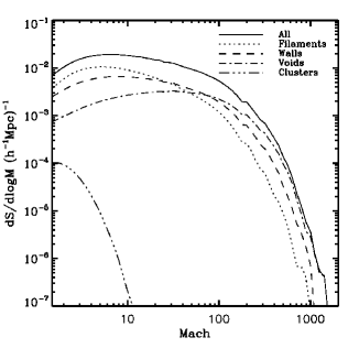
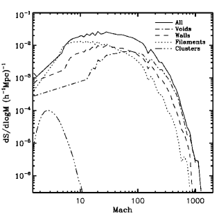
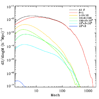
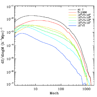
Figure 8: Differential shock surface area as a function of logarithmic Mach number bins. The top left panel shows the distribution for the different elements of the cosmic web: voids (dash-dotted line), walls (dashed line), filaments (dotted line) and clusters (dash-dot-dotted line). The solid line shows the combine distribution of all the elements of the cosmic web. By applying the deconvolution technique (Sect. 6) to these distributions, we obtained the results presented in the top right panel. The bottom left panel shows the shock surface distribution divided into several ranges of overdensity. The bottom right panel shows the distribution divided into several temperature ranges.

We also construct the differential shock surface area in terms of temperature and density, in order to compare with Skillman et al. (2008). This is shown in the lower panels of Fig. 8. The difference between these panels and the upper panels is that here we divide the shock surface area in temperature and density ranges. The temperature and density ranges are intended to denote the different temperature and density of the elements of the cosmic web. for simplicity, we do not deconvolve these distributions. When looking at density cuts (lower left panel of Fig. 8), it is interesting to notice that cluster cores ($\delta>10^{4}$) have low Mach numbers and low surface area. This is mainly due to the fact that this region has already been heated, and so its temperature is high. Low-density regions ($\delta<1$) may be associated with voids. These regions have high characteristic Mach numbers due to their low density and low temperature. We see that there is an increase of the characteristic Mach number as the density decreases.

Similar results are observed when looking at the temperature cuts. Each cut has a characteristic Mach number, which increases as temperature decreases. For high temperature ($T>10^{7}$ K), the characteristic Mach number is $\mathcal{M}_{\mathrm{char}}\approx 2$, while for $T<1000$ K, $\mathcal{M}_{\mathrm{char}}\approx 20$. Skillman et al. (2008) states that this characteristic Mach number is due to the maximum temperature jump possible for a given temperature.

In general, we find good agreement with the result of Skillman et al. (2008) for cuts with low density and temperature. For dense structures we find that our results differ significantly from Skillman et al. (2008). More precisely, we find that even in regions with $\delta>10^{3}$ shocks with $\mathcal{M}\gtrsim 100$ can be found, while Skillman et al. (2008) find that shocks have Mach numbers basically below 10 for regions with $\delta>10^{3}$. Comparing the density cuts (lower left panel of Fig. 8) with the upper panels we see that dense regions with high Mach number does not reside in clusters. Instead, these are dense structures in filaments, walls or voids. The particle based TreeSPH simulation technique, as used in Gadget, tends to from clumpy structures. Therefore, we find dense structures with $\delta>10^{3}$ even outside of clusters. If these structures reside close to an accretion shock, we find a high Mach number at a relatively high density. This effect is enhanced by smearing out shock fronts in SPH by approximately two times the smoothing length.

For region with $\delta>10^{4}$ we find significantly less shocks than Skillman et al. (2008). The difference is likely caused by a lower effective resolution in our SPH simulation. Skillman et al. (2008) used a simulation box with a side length of $512\,h^{-1}\,{\rm Mpc}$. They used a root grid resolution for both dark mater and gas of 512. For dark matter the MareNostrum simulation is significantly better resolved. In the AMR scheme with a density refinement criterium the resolution follows the mass roughly in a similar way as SPH. However, since the SPH kernel smoothes over $N$ particles (64 in our case), the effective resolution for gas is in the MareNostrum simulation by a factor of 2 lower than in the ’Santa Fe Light Cone’ used by Skillman et al. (2008). A higher resolution as used in the MareNostrum simulation is necessary to form shock fronts in regions with $\delta>10^{4}$.

7.2 Temperature Distribution and Physical Properties of the Cosmic Web

As mentioned earlier, one of the big advantages of the SpineWeb procedure is that we can precisely characterize the different elements of the cosmic web. We can, therefore, study the temperature and density distribution in the different elements of the cosmic web.

Table 2: Mean temperature and mean density contrast of the different elements of the cosmic web at $z=0$.

	$\langle\mathrm{T}\rangle$ (K)	$\sigma_{T}$	$\langle\delta\rangle$	$\sigma_{\delta}$
Clusters	7.90$\times 10^{7}$	8.13$\times 10^{7}$	885.73	1108.28
Filaments	7.30$\times 10^{6}$	1.44$\times 10^{7}$	71.87	180.27
Walls	2.21$\times 10^{6}$	6.84$\times 10^{6}$	18.71	71.24
Voids	6.96$\times 10^{5}$	4.30$\times 10^{6}$	2.89	25.17

Table 2 shows the mean values of the temperature and density contrast of the MareNostrum simulation. The shown temperature is the simulation temperature corrected using the relation in Eqn. 12. The mean values were obtained by averaging the temperature and density of the particles that belong to the different environments. As expected, clusters are the hottest structures in the Universe, with a mean temperature of $7.90\times 10^{7}$ K. This is because clusters have deep potential wells into which baryons accrete, thus heating the clusters.

The most salient features of the cosmic web are the large filamentary networks which are interconnected across vast distances. The filamentary network permeates all regions of space, even the underdense voids. We find that filaments have a mean temperature of $7.30\times 10^{6}$ K, which is well within the range estimated for the filamentary WHIM temperature ($10^{5}-10^{7}$ K).

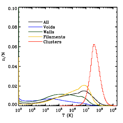
Figure 9: Temperature distribution of the different environments of the Cosmic Web.

Table 2 also shows the density contrast of the constituents of the cosmic web. Filaments are the second densest objects in the Universe, with $\langle\delta\rangle\sim 70$. Walls are less dense than filaments, with $\langle\delta\rangle~{}\sim 19$. Finally, voids have a mean density contrast of $\langle\delta\rangle~{}\sim 3$.

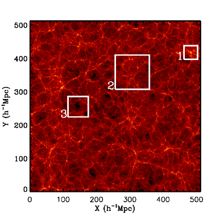
Figure 10: Density field of the MareNostrum Universe. The figures represents a slice of 20$h^{-1}$Mpc thick through the z-axis. Three elements are distinguished: the most massive cluster in the simulation (box number 1), a region of rich filaments (box number 2) and a void region (box number 3). The different environments were find using the SpineWeb technique.

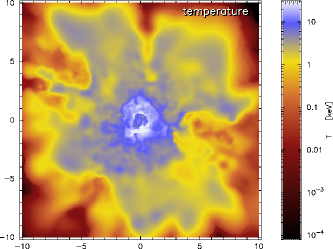
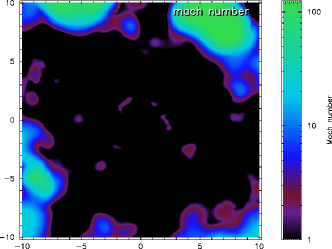
Figure 11: Temperature and Mach number in an infinitesimally slice for the most massive cluster in the MareNostrum simulation (box 1 in Fig. 10).

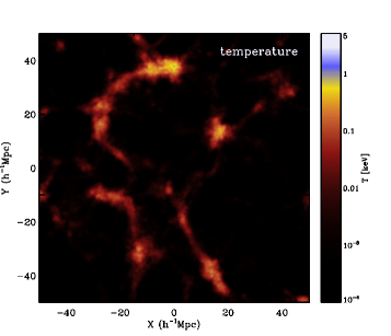
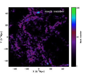
Figure 12: Temperature and Mach number in a thin slice of a rich region of filaments in the MareNostrum simulation (box 2 in Fig. 10)

.

Fig. 13 depicts a zoom-in of box number 3 of Fig. 10. As in the previous figure, we only consider void particles as defined by the SpineWeb procedure. Interesting is to notice that voids are not empty. As mentioned before, Gottlöber et al. (2003) stated that voids are like miniature universes. Voids have what may be called sub-walls and sub-filaments (a sub-network), with void galaxies the nodes of the sub-filaments. These sub-walls and sub-filaments do not have a high enough density to be considered walls or filaments on their own. In the region chosen, of 60$h^{-1}$Mpc on a side, we see what it could be void galaxies and some tenuous filamentary structure. The temperature of this region is $T\approx\times 10^{3}-10^{6}$. We see that a void region has high Mach numbers mainly due to the low temperature of the accreting gas. We find that void regions in the MareNostrum simulation have shocks with Mach numbers $\mathcal{M}\gtrsim 1000$. However, these high Mach numbers may not be real, and they may be due to the low temperature floor set in the simulation (see Section 7.1).

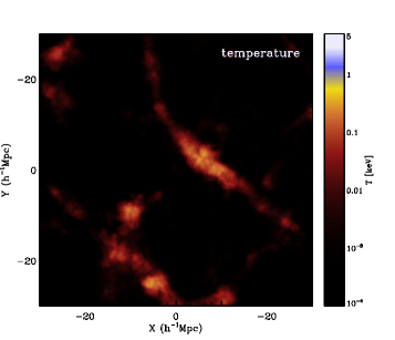
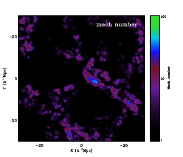
Figure 13: Temperature and Mach number in a 10$h^{-1}$Mpc thick slice for a void region (box 3 in Fig. 10).

7.3 Radio Emission in the Cosmic Web

Each SPH particle has been assigned a radio luminosity via Eqn. 8 and with the correct setting of $f_{\mathrm{A}}(\mathcal{M})$ (Eqn. 11). With this in hand it is possible to construct artificial radio maps. To this end, we project the emission of each particle long the line of sight and smooth it with the SPH kernel size. The radio emission is computed for an observing frequency of 1.4 GHz and a hypothetical beam of 10$\times$10 arcsec². For comparison, we also compute contours of the bolometric X-ray flux. Each SPH particle is assigned a luminosity (Navarro et al., 1995)

$$L_{X}\,=\,1.2\times 10^{-24}\mathrm{ergs^{-1}}\frac{m_{\mathrm{gas}}}{\mu m_{\mathrm{p}}}\frac{n_{e}}{\mathrm{cm^{-3}}}\left(\frac{T}{keV}\right)^{1/2}\,.$$ (13)

We will study the radio emission in each component of the cosmic web. The results in these section are obtained using an electron efficiency of $\xi_{\mathrm{e}}=0.005$. In Section 7.4 we calibrate our simulated data against observations, yielding a different electron efficiency and, therefore, different number of radio objects.

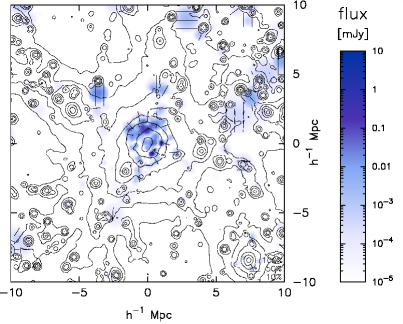
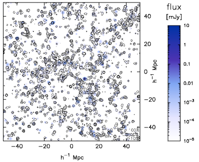
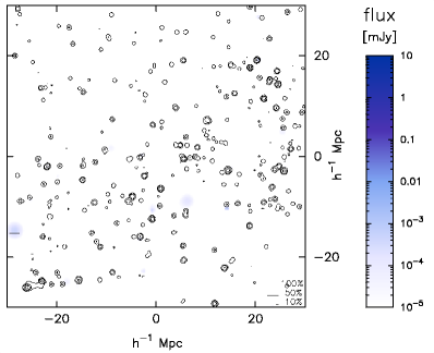
Figure 14: Synthetic observations of X-ray and radio emission. The radio flux at 1.4 Ghz is computed for a hypothetical beam size of $10\times 10$ arcsec². Upper panel: the galaxy cluster depicted in Fig. 11. Middle panel: the filamentary region shown in Fig. 12. Bottom panel: the void region shown in Fig. 13. The thin straight lines indicate the direction of polarization. The length of the line indicates the degree of polarization.

7.3.1 Clusters

Of the total sample of galaxy clusters present in the MareNostrum Universe ($\sim 3800$) we find that only $565$ cluster of galaxies have radio objects ($693$) with $P_{1.4}>10^{30}$ ergs s^-1 Hz^-1 (see Sec.  for a correction on this number based on a correction of $\xi_{\mathrm{e}}$). This represents only $\sim 15\%$ of the total galaxy cluster sample. In total, we find that $\sim 41\%$ of the total sample of galaxy clusters host diffuse radio emission. These clusters are not necessarily the most massive ones, but they are within the entire mass range.

Fig. 14 shows the synthetic observation of X-ray and radio emission of the most massive cluster in the simulation. The thin straight lines in the maps indicate the direction of polarization. The length of the line indicates the degree of polarization. For comparison the length corresponding to 10%, 50% and 100% is shown. The polarization is computed according to the formalism described in (Burn, 1966) and (Enßlin et al., 1998). The radio emission is caused by internal shock fronts in the clusters. We could, therefore, exclude external shocks as sources for producing radio emission in cluster (see also Hoeft et al. 2008). We find that clusters host the majority of radio objects, with $\sim 20-30$ objects with $P_{1.4}>10^{32}$ ergs s^-1 Hz^-1 (see Section 7.4). Of a total of $\sim 1500$ radio objects with $L_{R}>P_{1.4}>10^{30}$ ergs s^-1 Hz^-1 found in the simulation, $\sim 500$ are located in galaxy clusters, i.e., 33% of the total radio objects.

We also estimate the relation between the radio luminosity, $P_{1.4}$, of the radio objects and the emission weighted temperature of its galaxy clusters hosts. This result should be similar to the one obtained by Hoeft et al. (2008), only that our sample of galaxy clusters is 10 times larger than theirs.

Fig. 15 shows that those clusters that host the very luminous radio objects, i.e., $P_{1.4}>10^{32}$ ergs s^-1 Hz^-1, are very hot ($T_{X}>8$ keV)., i.e., very massive. As was also pointed out by Feretti et al. (2004), there is a correlation between the radio luminosity of the radio objects and the temperature of its host cluster, i.e., the hottest clusters hosts the most luminous radio objects.

Our results are quite similar to those presented in Hoeft et al. (2008). This is expected since their sample is a fraction of the sample of clusters presented here. The results presented here reinforce that our simple emission model recreate diffuse radio emission not only in galaxy clusters, but also in the cosmic web, and picks up the trend in the radio luminosity - X-ray relation.

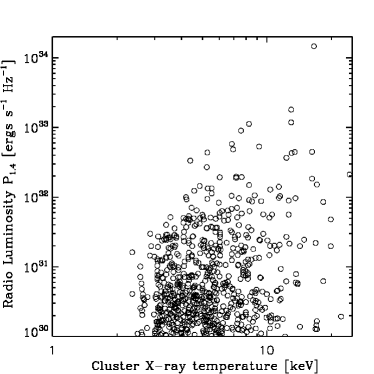
Figure 15: Radio luminosity of radio objects versus the emission weighted temperature of galaxy clusters.

7.3.2 Filaments

Bagchi et al. (2002) reported the existence of a large-scale diffuse radio emission from a large-scale filamentary network. Kim et al. (1989) also suggested the presence of diffuse radio emission in the Coma Supercluster. Temperatures of filaments are in the range $T\approx 10^{5}-10^{7}$, and magnetohydrodynamic simulations (MHD) estimate a magnetic field that varies from $10^{-1}$ nG to $10$ nG (Sigl et al., 2003; Brüggen et al., 2005). This is in line with Ryu et al. (2008), who suggest an average magnetic strength to be of the order of $10$ nG. However, Bagchi et al. (2002) estimated that the strength of the magnetic field in the filamentary network is $B\approx 0.3-0.5$ $\mu$G. In the same line, Dolag et al. (2005) suggests the strength of the magnetic field of filaments that connect galaxy clusters to be as large as $0.1$ $\mu$G. The middle panel of Fig. 14 shows the synthetic observations of the X-ray and the radio emission for the filamentary region shown in Fig. 12. We found that filaments show diffuse radio emission, especially in areas near to cluster of galaxies. However, although filaments have strong Mach numbers (see Fig. 12), the flux in ”pure” filamentary regions, i.e., regions far from the outskirts of clusters is low, as seen in Fig. 14, and may not be detectable with the upcoming radio telescopes.

As for the number of radio objects, we find that filaments host fewer radio objects than clusters, with $\sim 2-3$ radio objects with $P_{1.4}>10^{32}$ ergs s^-1 Hz^-1 (see Section 7.4).

7.3.3 Voids

As discussed in Sect. 5, esitmation of magnetic field outside galaxy clusters is difficult. Moreoever, MHD simulations have not been conclusive as well, assigning a magnetic field that varies from $10^{-3}$ nG to $10^{-1}$ nG (Sigl et al., 2003). Further studies on the magnetic field on voids are necessary to precisely determine the strength of these magnetic fields.

As can be seen in the bottom panel of Fig. 14, there are some areas in the void region that shows a very tenuous radio emission, with fluxes $\lesssim 10^{-4}$ mJy. This is basically due to two facts: temperatures in voids, as we have seen, is very low compared to the other components of the cosmic web. It has also been suggested that the magnetic field in voids is quite low. Although observationally it has been possibly to estimate the magnetic field in clusters of galaxies (e.g., Bonafede et al., 2010), this has not been possible for voids.

7.4 Radio objects luminosity function

As we have shown, there exists the possibility of finding radio emission in other environments of the cosmic web, such as filaments. We now turn our attention to the possibility of finding individual radio objects in the cosmic web. We do this in a similar way to that of Hoeft et al. (2008), with a slight difference. We select all particles whose radio emission lies above a very low threshold. This threshold corresponds roughly to particles with $\mathcal{M}\gtrsim 2$. Instead of finding their nearest neighbor and link them according to their smoothing length, as done by Hoeft et al. (2008), we use HOP to link the particles and find individual groups. This is a somewhat simpler approach, but given that HOP works on a density basis, it assures us that the particles will form a compact group. Having found the groups, we compute the cumulative number of radio objects above a given luminosity, that is, the luminosity function of diffuse radio objects.

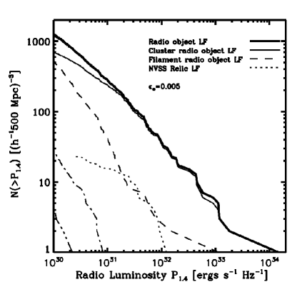
Figure 16: Cumulative number density of radio objects. The thick solid line indicates the total number of radio objects in the simulation box. The thin solid line shows the number of radio objects within clusters. The dashed line indicates the radio objects present in filaments. The dashed-dotted line depicts the radio objects in walls, while the dashed-dotted-dashed line represent the radio objects present in voids. For comparison, the NVSS relic luminosity function (dotted line).

Fig. 16 shows the radio luminosity function for radio objects in the simulation box. For comparison, we also show a radio relic luminosity function constructed with relic data observations (Giovannini et al., 1999; Govoni et al., 2001; Bonafede et al., 2009; Clarke & Ensslin, 2006; Feretti et al., 2006; Bagchi et al., 2006; Röttgering et al., 1997; van Weeren et al., 2009; Feretti et al., 2001; Giacintucci et al., 2008; Venturi et al., 2007). Most of these data were obtained from the NRAO VLA Sky Survey (NVSS) (Condon et al., 1998).

We see that with our simple assumptions, we find a much larger number of radio objects in the entire simulation box. Also, if we compare with our cluster radio object luminosity function (thin solid line), we still find more radio objects. Galaxy clusters host the majority and the most luminous objects, with $\sim 34$ objects with $P_{1.4}>10^{32}$ ergs s^-1 Hz^-1. Filaments also host some radio objects, but most of them are less luminous, with only a couple with $P_{1.4}>10^{32}$ ergs s^-1 Hz^-1. Finally, walls and voids also host a few radio objects, but they are rather weak. Table 3 shows the fraction of radio objects by environment for different total radio luminosity ranges. It can be seen that clusters host the majority of more luminous radio objects ($P_{1.4}>10^{32}$ ergs s^-1 Hz^-1), but when considering the complete sample of radio objects, these are located within filaments. This is to expect, since a great part of the mass of the Universe resides in filaments (Aragón-Calvo et al., 2010b). This is also an indication that the detection of diffuse radio emission in filaments could shed light on the missing-baryon problem. Walls also host a great number of low-luminous radio objects, while in voids the presence of radio objects is negligible.

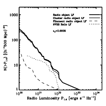
Figure 17: Same as Fig. 16, but the total radio power has been rescaled by using a electron efficiency parameter of $\epsilon_{e}=0.0005$. By doing this, radio objects are less luminous, and we are able to match our simulated relics with observational NVSS relics.

As pointed out by Hoeft et al. (2008), the overestimation of radio objects may be due to an overestimation of the electron efficiency ($\xi_{\mathrm{e}}$), as well as the magnetic fields. The value of the the electron efficiency parameter is quite uncertain from current observational and theoretical constrains (Skillman et al., 2010). From Eqn. 8, we see that the relationship between the total radio power and $\xi_{\mathrm{e}}$ is linear, so in order to obtain less luminous objects, we just have to rescaled the total radio power, e.g., an electron efficiency of $\xi_{\mathrm{e}}=0.0005$ will lead to a total radio power that is low by a factor of 10. In order to match our results to observations, i.e., the NVSS radio relic luminosity function, we rescale the luminosity function using $\epsilon_{e}=0.0005$, shown in Fig. 17. As expected, radio objects are less luminous, and therefore, less radio objects are found. In the plotted range, there are no radio objects in voids and filaments, only 1 in filaments, and some group of ten in clusters. With this electron efficiency, the cluster radio objects matches the observational NVSS radio relic luminosity function (see Fig. 17). However, we predict more relics at the high and low power compared with the observed function. This can be to due to the fact that the observed relics, to date, is still small, compared to the large number of relics found in the simulation with our method. Upcoming radio observations will increase the number of observed relics, making the statistics stronger. Table 3 shows the fraction of radio objects by environment for different total radio luminosity ranges with the adjusted electron efficiency parameter. A study of the effects of the magnetic fields is beyond the scope of this paper, so we do not investigate this.

The luminosity function (Eqn. 16) suggest what can be expected with the use of the upcoming radio telescopes. An increase of the surface brightness sensitivity by a factor of 10 will result in an increase of the number of radio objects by a factor of 10-100 (see also Skillman et al. (2010). We can also estimate the number of radio objects to be found in a given survey area and redshift depth by solving the equation:

$$\frac{dV}{dzd\Omega}(z)\,=\,D_{H}\frac{(1+z)^{2}D^{2}_{A}}{E(z)}\,,$$ (14)

where $D_{H}\equiv c/H_{0}$ is the Hubble distance, $D_{a}$ is the angular diameter distance and $E(z)=\sqrt{\Omega_{m}(1+z)^{3}+\Omega_{k}(1+z)^{2}+\Omega_{\Lambda}}$. For a flat, $\Lambda$-dominated Universe like the MareNostrum simulation, $\Omega_{k}=0$ and Eqn. 14 can be rewritten as (Carroll et al., 1992)

$$V_{C}\,=\,\frac{4\pi}{3}D_{M}^{3}\,,$$ (15)

where $D_{M}$ is the comoving distance, which, for a flat Universe, coincides with the line-of-sight comoving distance. Eqn. 15 corresponds to the total comoving volume in an all-sky survey out to redshift $z$. For the MareNostrum Universe, the result of Eqn. 14 corresponds to an all-sky survey out to $z\sim 0.18$. If we assume an electron efficiency of $\xi_{\mathrm{e}}=0.005$ ($\xi_{\mathrm{e}}=0.0005$), we expect to find 34 (4) radio objects in 30 (3) galaxy clusters, 2 (1) radio objects in filaments and none in walls and voids, all with a total radio luminosity of $P_{1.4}>10^{32}$ ergs s^-1 Hz^-1 within this cosmological volume. Assuming that the number density of radio objects is nearly constant through cosmic time (Skillman et al., 2010), we could estimate that in an all-sky survey out to $z=0.5$ (which corresponds to a volume of $\sim 15$ times the previous one), we could find 510 (60) radio objects in 450 (45) clusters, 30 (15) radio objects in filaments and a few in walls and voids.

Table 3: Fraction of total radio objects ($\sim 14600$) with a given radio luminosity $P_{1.4}$ in terms of their environment assuming an electron efficiency of $\xi_{\mathrm{e}}=0.005$ ($\xi_{\mathrm{e}}=0.0005$) Units of radio luminosity given in ergs s^-1 Hz^-1.

	$P_{1.4}>10^{32}$	$10^{30}<P_{1.4}\leq 10^{32}$	$P_{1.4}<10^{30}$
Clusters	0.23% (0.03%)	4.51% (1.6%)	10.33% (13.46%)
Filaments	0.01% (0%)	3.65% (0.3%)	74.24% (77.58%)
Walls	0% (0%)	0.18% (0%)	6.40% (6.58%)
Voids	0% (0%)	0.03% (0%)	0.42% (0.45%)

The use of the SpineWeb enable us to make predictions of the radio flux in filaments. Assuming an spectral index of $\alpha=1$, filaments at a redshift $z\sim 0.15$, in a frequency of 150 MHz, a radio flux of $S_{150MHz}\sim 0.12$ $\mu$Jy.

8 Conclusions

We have analyzed one of the largest hydrodynamical simulations of cosmic structure formation, namely the MareNostrum simulation, with the purpose of studying the possibility of detecting radio emission in the cosmic web. To that purpose, we use: i) a novel method for estimating the radio emission of strong shocks that occur during the process of structure formation in the Universe developed by Hoeft & Brüggen (2007) and ii) the SpineWeb technique The SpineWeb procedure deals with the topology of the underlying density field, correctly identifying voids, walls and filaments. While previous studies focused on the study of cosmological shocks in selected catalogs of galaxy clusters or by defining the different environments of the cosmic web by density and/or temperature cuts, we are able to correctly disentangle the complex filamentary network of the cosmic web. The computation of the radio emission is based on an estimate for the shock surface area. The radio emission is computed per surface area element using the Mach number of the shock and the downstream plasma properties.

In order to properly calculate the radio emission, two corrections were made. The first correction deals with the shock surface area. The constant area factor ($f_{a}$) of Eqn. 8 was corrected using shock tube tests and a convolution method described in Appendix A. One deals with the temperature of the simulation. Given that the simulation was run with a low floor temperature and without UV background, expansion cooling leads to very low temperature, which leads to very high Mach numbers. We corrected this by scaling the temperature of cold, low density regions using $T=T_{0}(1+\delta)^{\gamma-1}$ (Hui & Gnedin, 1997), where $\delta$ is the overdensity. The first step was to calculate the strength of cosmological shocks, characterized by their Mach number using the method described in Hoeft et al. (2008). We find that each environment of the cosmic web has a distinct Mach distribution: voids have a characteristic Mach number of $\mathcal{M}_{\mathrm{voids}}\approx 18$; walls, $\mathcal{M}_{\mathrm{walls}}\approx 7.5$; filaments, $\mathcal{M}_{\mathrm{filaments}}\approx 6.2$; and clusters, $\mathcal{M}_{\mathrm{clusters}}\approx 1.8$. The strength of the shock, i.e., the characteristic Mach number, is closely related to the temperature and density of the medium. Voids are the coldest and less dense region in the Universe, with a mean temperature $\langle\mathrm{T}\rangle_{\mathrm{voids}}\approx 7\times 10^{5}$ K and $\langle\delta\rangle_{\mathrm{voids}}\approx 2.9$, and they interact with walls and filaments, which are denser and hotter structures, with filaments reaching a mean temperature of $\langle\mathrm{T}\rangle_{\mathrm{voids}}\approx 7.3\times 10^{6}$ K and $\langle\delta\rangle_{\mathrm{voids}}\approx 72$.

Applying a radio emission model based on DSA to the simulation we are able to reproduce the diffuse radio emission in galaxy clusters using a lower electron efficiency to that used by Hoeft et al. (2008). This diffuse radio emission is also present in filaments. In walls and voids the emission is very weak, resulting in almost no presence of radio objects. By identifying radio objects based on their density, we find that clusters hosts the majority of such objects. Assuming an electron efficiency of $\xi_{\mathrm{e}}=0.005$, we find that 30 galaxy clusters (out of 3865) host 34 radio objects with $P_{1.4}>10^{32}$ ergs s^-1 Hz^-1. If we consider a radio luminosity of $10^{30}<P_{1.4}\leq 10^{32}$ ergs s^-1 Hz^-1, then 659 radio objects are found in 547 galaxy clusters, only $\sim 15\%$ of the total sample. These radio objects are present in the entire mass range of the galaxy clusters, i.e., both low mass and high mass clusters present radio objects. Filaments also host radio objects, although only 2 of them are very luminous ($P_{1.4}>10^{32}$ ergs s^-1 Hz^-1). However, the majority of low luminous radio objects ($P_{1.4}<10^{30}$) are present in filaments. The presence of radio objects in walls and voids is rather negligible.

We calibrated our simulated data against the observational NVSS radio relic luminosity function, yielding an electron efficiency of $\xi_{\mathrm{e}}=0.0005$. This is a factor of 10 less than the one estimated by Hoeft et al. (2008). When using this efficiency, the number of very luminous radio objects drop dramatically. We only find 4 radio object with $P_{1.4}>10^{32}$ ergs s^-1 Hz^-1 and 1 in filaments. In the range $10^{30}<P_{1.4}\leq 10^{32}$ ergs s^-1 Hz^-1, we find 235 radio objects in 198 galaxy clusters (5% of the total sample) and 43 in filaments.

An all-sky survey up to $z=0.5$ and assuming an efficiency of $\xi_{\mathrm{e}}=0.005$ ( $\xi_{\mathrm{e}}=0.0005$) should result in the discovery of 510 (60) radio objects in 450 (45) clusters, and 30 (15) radio objects in filaments. With the increase of surface brightness sensitivity of the upcoming radio telescopes, the detection of radio objects should increase by a factor of 10, which opens in the possibility of finding a considerable number of radio objects in filaments. Furthermore, we predict that the radio flux of filaments at redshift $z\sim 0.15$, and at a frequency of 150 MHz, should be $S_{\small{150MHz}}\sim 0.12$ $\mu$Jy.

Appendix A Correcting the shock surface area distribution

Convolution is a mathematical operation on two functions, $f$ and $g$, which produces a third function that is a modified version of the one of the original functions. Usually, one of the two functions is taken to be a kernel function which acts on the other function, modifying it. The standard convolution states that

$$h(t)\,=\,f(t)\ast g(t)\,\equiv\,\int_{-\infty}^{\infty}f(\tau)g(t-\tau)d\tau\,,$$ (16)

where $\ast$ is the convolution operand. The inverse of this operation is called deconvolution. In our case, we have a measured distribution, namely $dS/d\log{\mathcal{M}}$, obtained from the simulation and we wish to obtain the real distribution, i.e., the shock surface area distribution taking into account the particles that were assign a low Mach number in strong shocks and the underestimation of the different Mach numbers. Therefore, we need to find the shock tube distribution kernel taken from the shock tubes data in order to deconvolve it with our measure function. However, instead of finding the inverse of the kernel function, we will iterate the convolution procedure, which will yield the real distribution. The convolution we want to solve is

$$q^{m}(\log{\mathcal{M}})\,=\,\int_{0}^{\infty}d\log{\mathcal{M}}^{\prime}f(\log{\mathcal{M}},\log{\mathcal{M}}^{\prime})q^{r}(\log{\mathcal{M}}^{\prime})\,,$$ (17)

where $q^{m}(\log{\mathcal{M}})$ is the measured shock surface distribution, $f(\log{\mathcal{M}},\log{\mathcal{M}}^{\prime})$ is the kernel function and $q^{r}(\log{\mathcal{M}})$ is the real distribution we want to find. In Eqn. 17 we have taken two things into account: i) there are not negative Mach numbers, and ii) the kernel function depends on the Mach number.

In Section 6 we saw that a simple representation to the shock surface area of the shock tubes are a Heaviside function and a Gaussian. Therefore, our kernel has the form

$$\mathbf{F}(\log{\mathcal{M}})_{ij}\,=\,\mathcal{K}\cdot\mathcal{H}(\log{\mathcal{M}}_{i})+\mathcal{G}_{ij}(\log{\mathcal{M}}_{i},\log{\mathcal{M}}_{j})\,,$$ (18)

where $\mathcal{G}_{ij}$ is a Gaussian with form

$$\mathcal{G}_{ij}\,=\,e^{-(\log{\mathcal{M}}-\log{\mathcal{M}^{\prime}})^{2}/2\sigma(\log{\mathcal{M}^{\prime}})^{2}}\,,$$ (19)

where the standard deviation also depends on the measured Mach numbers, i.e., $\sigma=\sigma(\log{\mathcal{M}})$ as seen in the previous section.

After constructing the kernel with the fitting parameters of the various shock tubes, we give a guess function in order to start the iteration procedure. As a first guess, we choose $q^{r}_{1}=q^{m}$, and convolve that with the kernel, giving as a result $q^{m}_{1}$. The new guess is then calculated by subtracting the previous guess with the difference between the result of the convolution of the first guess with the measured function, i.e., $q^{r}_{2}=q^{r}_{1}-(q^{m}_{1}-q^{m})$. We found that after iterating 5 times we are able to recover $q^{m}$.

References

- Aragón-Calvo et al. (2010a) Aragón-Calvo, M. A., Platen, E., van de Weygaert, R., & Szalay, A. S. 2010a, ApJ, 723, 364
- Aragón-Calvo et al. (2010b) Aragón-Calvo, M. A., van de Weygaert, R., & Jones, B. J. T. 2010b, MNRAS, 408, 2163
- Aragón-Calvo et al. (2010c) Aragón-Calvo, M. A., van de Weygaert, R., Araya-Melo, P. A., Platen, E., & Szalay, A. S. 2010c, MNRAS, 404, L89
- Bagchi et al. (2002) Bagchi, J., Enßlin, T. A., Miniati, F., Stalin, C. S., Singh, M., Raychaudhury, S., & Humeshkar, N. B., 2002, New Astronomy, 7, 249
- Bagchi et al. (2006) Bagchi, J., Durret, F., Neto, G. B. L., & Paul, S., 2006, Science, 314, 791
- Battaglia et al. (2009) Battaglia, N., Pfrommer, C., Sievers, J. L., Bond, J. R., & Enßlin, T. A., 2009, MNRAS, 393, 1073
- Berrington & Dermer (2003) Berrington, R. C., & Dermer, C. D., 2003, ApJ, 594, 709
- Beucher & Lantuejoul (1979) Beucher S., Lantuejoul C., 1979, in Proceedings International Workshop on Image Processing, CCETT/IRISA, Rennes, France
- Bonafede et al. (2009) Bonafede, A., Giovannini, G., Feretti, L., Govoni, F., & Murgia, M., 2009, A&A, 494, 429
- Bonafede et al. (2010) Bonafede, A., Feretti, L., Murgia, M., Govoni, F., Giovannini, G., Dallacasa, D., Dolag, K., & Taylor, G. B. 2010, A&A, 513, A30
- Bond et al. (1996) Bond, J. R., Kofman, L., & Pogosyan, D., 1996, Nature, 380, 603
- Brüggen et al. (2005) Brüggen, M., Ruszkowski, M., Simionescu, A., Hoeft, M., & Dalla Vecchia, C. 2005, ApJL, 631, L21
- Burn (1966) Burn, B. J. 1966, MNRAS, 133, 67
- Carroll et al. (1992) Carroll, S. M., Press, W. H., & Turner, E. L. 1992, ARA&A, 30, 499
- Cassano et al. (2010) Cassano, R., Ettori, S., Giacintucci, S., Brunetti, G., Markevitch, M., Venturi, T., & Gitti, M. 2010, ApJL, 721, L82
- Cen & Ostriker (2006) Cen, R., & Ostriker, J. P., 2006, ApJ, 650, 560
- Clarke & Ensslin (2006) Clarke, T. E., & Ensslin, T. A. 2006, ApJ, 131, 2900
- Colless et al. (2003) Colless, M., et al., 2003, arXiv:astro-ph/0306581
- Condon et al. (1998) Condon, J. J., Cotton, W. D., Greisen, E. W., Yin, Q. F., Perley, R. A., Taylor, G. B., & Broderick, J. J. 1998, ApJ, 115, 1693
- Davé et al. (2001) Davé, R., et al., 2001, ApJ, 552, 473
- Dolag et al. (2008) Dolag, K., Bykov, A. M., & Diaferio, A. 2008, SSRv, 134, 311
- Dolag et al. (2005) Dolag, K., Grasso, D., Springel, V., & Tkachev, I. 2005, J. Cosmology Astropart.Phys., 1, 9
- Eisenstein & Hut (1998) Eisenstein D. J., Hut P., 1998, ApJ, 498, 137
- Enßlin et al. (2007) Enßlin, T. A., Pfrommer, C., Springel, V., & Jubelgas, M., 2007, A&A, 473, 41
- Enßlin et al. (1998) Ensslin, T. A., Biermann, P. L., Klein, U., & Kohle, S. 1998, A&A, 332, 395
- Feretti et al. (2001) Feretti, L., Fusco-Femiano, R., Giovannini, G., & Govoni, F. 2001, A&A, 373, 106
- Feretti et al. (2004) Feretti, L., Burigana, C., & Enßlin, T. A. 2004, New A. Rev., 48, 1137
- Feretti et al. (2006) Feretti, L., Bacchi, M., Slee, O. B., Giovannini, G., Govoni, F., Andernach, H., & Tsarevsky, G. 2006, MNRAS, 368, 544
- Feretti & Giovannini (2008) Feretti, L., & Giovannini, G., 2008, in A Pan-Chromatic View of Clusters of Galaxies and the Large-Scale Structure, ed. M. Plionis, O. Lopez-Cruz, D. Hughes, Lect. Notes Phys., 740, 143 (Springer)
- Gabici & Blasi (2003) Gabici, S., & Blasi, P., 2003, ApJ, 583, 695
- Giacintucci et al. (2008) Giacintucci, S., et al., 2008, A&A, 486, 347
- Giovannini et al. (1999) Giovannini, G., Tordi, M., & Feretti, L. 1999, New A., 4, 141
- Giovannini et al. (2006) Giovannini, G., Feretti, L., Govoni, F., Murgia, M., & Pizzo, R., 2006, Astronomische Nachrichten, 327, 563
- Gottlöber et al. (2003) Gottlöber, S., Łokas, E. L., Klypin, A., & Hoffman, Y. 2003, MNRAS, 344, 715
- Gottlöber & Yepes (2007) Gottlöber, S., & Yepes, G., 2007, ApJ, 664, 117
- Govoni et al. (2001) Govoni, F., Feretti, L., Giovannini, G., Böhringer, H., Reiprich, T. H., & Murgia, M. 2001, A&A, 376, 803
- Hoeft & Brüggen (2007) Hoeft, M., & Brüggen, M. 2007, MNRAS, 375, 77
- Hoeft et al. (2008) Hoeft, M., Brüggen, M., Yepes, G., Gottlöber, S., & Schwope, A. 2008, MNRAS, 391, 1511
- Hui & Gnedin (1997) Hui, L., & Gnedin, N. Y. 1997, MNRAS, 292, 27
- Jubelgas et al. (2008) Jubelgas, M., Springel, V., Enßlin, T., & Pfrommer, C., 2008, A&A, 481, 33
- Kang et al. (2005) Kang, H., Ryu, D., Cen, R., & Song, D., 2005, ApJ, 620, 21
- Kardashev (1962) Kardashev, N. S. 1962, Soviet Astronomy, 6, 317
- Keshet et al. (2003) Keshet, U., Waxman, E., Loeb, A., Springel, V., & Hernquist, L., 2003, ApJ, 585, 128
- Kim et al. (1989) Kim, K.-T., Kronberg, P. P., Giovannini, G., & Venturi, T. 1989, Nature, 341, 720
- Klypin et al. (2001) Klypin A., Kravtsov A. V., Bullock J. S., Primack J. R., 2001, ApJ, 554, 903
- Markevitch et al. (2005) Markevitch, M., Govoni, F., Brunetti, G., & Jerius, D., 2005, ApJ, 627, 733
- Markevitch (2006) Markevitch, M., 2006, The X-ray Universe 2005, 604, 723
- Meli & Biermann (2006) Meli, A., & Biermann, L. P., 2006, Nuclear Physics B Proceedings Supplements, 151, 501
- Miniati et al. (2000) Miniati, F., Ryu, D., Kang, H., Jones, T. W., Cen, R., & Ostriker, J. P., 2000, ApJ, 542, 608
- Miniati et al. (2001) Miniati, F., Jones, T. W., Kang, H., & Ryu, D., 2001, ApJ, 562, 233
- Miniati (2002) Miniati, F., 2002,
- Navarro et al. (1995) Navarro, J. F., Frenk, C. S., & White, S. D. M. 1995, MNRAS, 275, 720
- Platen et al. (2007) Platen, E., van de Weygaert, R., & Jones, B. J. T. 2007, MNRAS, 380, 551
- Pfrommer et al. (2006) Pfrommer, C., Springel, V., Enßlin, T. A., & Jubelgas, M., 2006, MNRAS, 367, 113
- Pfrommer et al. (2007) Pfrommer, C., Enßlin, T. A., Springel, V., Jubelgas, M., & Dolag, K., 2007, MNRAS, 378, 385
- Pfrommer et al. (2008) Pfrommer, C., Enßlin, T. A., & Springel, V., 2008, MNRAS, 385, 1211
- Roettiger et al. (1999) Roettiger, K., Burns, J. O., & Stone, J. M. 1999, ApJ, 518, 603
- Röttgering et al. (1997) Röttgering, H. J. A., Wieringa, M. H., Hunstead, R. W., & Ekers, R. D., 1997, MNRAS, 290, 577
- Ryu et al. (2003) Ryu, D., Kang, H., Hallman, E., & Jones, T. W., 2003, ApJ, 593, 599
- Ryu et al. (2008) Ryu, D., Kang, H., Cho, J., & Das, S. 2008, Science, 320, 909
- Sarazin (1999) Sarazin, C. L., 1999, ApJ, 520, 529
- Schaap & van de Weygaert (2000) Schaap, W. E., & van de Weygaert, R., 2000, A&A, 363, L29
- Schaap (2007) Schaap, W. E., 2007, The Delaunay Tessellation Field Estimator, Ph.D. Thesis, University of Groningen
- Sheth & van de Weygaert (2004) Sheth, R. K., & van de Weygaert, R. 2004, MNRAS, 350, 517
- Sigl et al. (2003) Sigl, G., Miniati, F., & Ensslin, T. A. 2003, Phys. Rev. D, 68, 043002
- Skillman et al. (2008) Skillman, S. W., O’Shea, B. W., Hallman, E. J., Burns, J. O., & Norman, M. L., 2008, ApJ, 689, 1063
- Skillman et al. (2010) Skillman, S. W., Hallman, E. J., O’Shea, B. W., Burns, J. O., Smith, B. D., & Turk, M. J., 2010, arXiv:1006.3559
- Sod (1978) Sod, G. A. 1978, Journal of Computational Physics, 27, 1
- Solovyeva et al. (2008) Solovyeva, L., Anokhin, S., Feretti, L., Sauvageot, J. L., Teyssier, R., Giovannini, G., Govoni, F., & Neumann, D., 2008, A&A, 484, 621
- Springel (2005) Springel V., 2005, MNRAS, 364, 1105
- Tegmark et al. (2004) Tegmark, M., et al., 2004, ApJ, 606, 702
- van de Weygaert & van Kampen (1993) van de Weygaert, R., & van Kampen, E. 1993, MNRAS, 263, 481
- van de Weygaert & Platen (2009) van de Weygaert, R., & Platen, E. 2009, arXiv:0912.2997
- van de Weygaert & Schaap (2009) van de Weygaert, R., & Schaap, W. 2009, Data Analysis in Cosmology, 665, 291
- van Weeren et al. (2009) van Weeren, R. J., Röttgering, H. J. A., Brüggen, M., & Cohen, A., 2009, A&A, 505, 991
- Vazza et al. (2009) Vazza, F., Brunetti, G., & Gheller, C., 2009, MNRAS, 395, 1333
- Venturi et al. (2007) Venturi, T., Giacintucci, S., Brunetti, G., Cassano, R., Bardelli, S., Dallacasa, D., & Setti, G. 2007, A&A, 463, 937
- Zel’Dovich (1970) Zel’Dovich, Y. B. 1970, A&A, 5, 84