Benchmarks of the full configuration interaction, Monte Carlo shell model, and no-core full configuration methods

Abstract

We report no-core solutions for properties of light nuclei with three different approaches in order to assess the accuracy and convergence rates of each method. Full configuration interaction (FCI), Monte Carlo shell model (MCSM), and no core full configuration (NCFC) approaches are solved separately for the ground state energy and other properties of seven light nuclei using the realistic JISP16 nucleon-nucleon interaction. The results are consistent among the different approaches. The methods differ significantly in how the required computational resources scale with increasing particle number for a given accuracy.

I Introduction and Motivation

Ab initio approaches to nuclear structure and reactions for $p$-shell nuclei have advanced significantly in the last few years GFMC ; NCSM12 ; CC . At the same time, fundamental approaches to the nucleon-nucleon ($NN$) and three-nucleon ($NNN$) interactions, such as meson-exchange theory and chiral effective field theory, have yielded major advances Wiringa:1994wb ; Pieper_3NF ; Illinois ; Epelbaum ; N3LO . Successful realistic $NN$ interactions from inverse scattering have also emerged Shirokov07 . These advances in microscopic nuclear theory combine to place serious demands on available computational resources for achieving converged properties of $p$-shell nuclei. In order to access a wider range of nuclei and experimental observables, while retaining predictive power, we require additional major advances in many-body methods.

These considerations motivate us to investigate the no-core Monte Carlo shell model (MCSM) which has advantageous scaling properties for accessing larger basis spaces and heavier nuclei. The MCSM was first introduced in Ref. Otuska_MCSM and we extend it here to treat systems without a core. In the present work we evaluate properties of a set of $p$-shell nuclei using the no-core MCSM and compare with exact results in the same single-particle basis from the full configuration interaction (FCI) method when feasible. We also compare with representative results from the full space ab initio no core full configuration (NCFC) Maris09_NCFC method. We adopt the JISP16 $NN$ interaction Shirokov07 without renormalization and without any $NNN$ interactions.

For each of the three many-body methods, all $A$ nucleons in the nucleus are treated on the same footing. Experimental observables are obtained from $A$-nucleon wave functions resulting from Hamiltonian diagonalization in the chosen many-body basis space. To perform the comparisons among the methods, we focus on ground state properties of seven nuclei as well as the properties of two low-lying narrow excited states.

For each method, we adopt the harmonic oscillator (HO) single-particle basis. We obtain eigensolutions of the nuclear intrinsic Hamiltonian expressed as a superposition of Slater determinants in the HO basis (FCI and NCFC) or the total angular momentum projected and parity projected deformed Slater determinants (MCSM). Neutron and proton orbitals are treated independently. The resulting calculated ground state energy is a rigorous upper bound on the exact result at any truncation. This upper bound character applies to the lowest calculated state of each total angular momentum and parity.

A major distinction among the methods is the definition of the cutoff that defines the finite many-body basis space in which the calculations are performed. All three methods should approach the exact solutions as the cutoffs are removed. Both the MCSM and the FCI methods employ a cutoff in the single-particle basis $N_{\mathrm{shell}}$ which is the highest shell of the symmetric three-dimensional HO that is included. All many-body basis states consistent with that cutoff are retained (FCI) or stochastically sampled (MCSM). On the other hand, the NCFC approach represents an extrapolation to the infinite matrix limit of a sequence of calculations in many-body basis spaces defined by a many-body basis cutoff $N_{\mathrm{max}}$, the maximum number of HO quanta included in a many-body basis state above the minimum for that nucleus.

A further distinction among the methods emerges from these different truncations — the NCFC approach may, in principle (though this is not used in the present benchmark), guarantee the factorization of the total wave function into an intrinsic (translationally invariant) part times a pure $0s$ HO for the center-of-mass (c.m.) motion whereas the MCSM and FCI approaches do not guarantee this factorization. The method of analysis introduced for the coupled cluster method CC_CM implies that MCSM and FCI may factorize reasonably well at an optimally chosen oscillator parameter so that observables may be evaluated with minimal influence from spurious c.m. motion effects. All other known symmetries of the intrinsic Hamiltonian are retained in the many-body basis by each method.

The main motivation for the no-core MCSM approach is its superior scaling properties with increasing nucleon number. We estimate that, for a fixed $N_{\mathrm{shell}}$ value and a fixed level of accuracy the MCSM scales as $N_{b}^{2}\times N_{\mathrm{sp}}^{3\sim 4}$ where $N_{b}$ is the number of Monte Carlo basis states generated in the sampling and $N_{\mathrm{sp}}$ is the number of HO single-particle states included by $N_{\mathrm{shell}}$. To obtain a fixed accuracy with increasing nucleon number $A$, $N_{b}$ will have to increase as some low power of $A$, estimated at $1.5\sim 2.5$ from the results we present below. Assuming $N_{b}$ dominates the $A$ dependence for fixed accuracy, which seems reasonable, we estimate that MCSM scales as $A^{3\sim 5}$. On the other hand, the NCFC scales as $A^{12\sim 14}$ for a fixed $N_{\mathrm{max}}$ value and the maximum $N_{\mathrm{max}}$ value roughly fixes the accuracy of the final NCFC result. Since the MCSM scaling for fixed accuracy is far less dependent on the number of nucleons $A$, it will be the superior approach once $A$ increases to the point where the NCFC fails to generate a sufficiently converged result. Nevertheless, the truncated calculations within NCFC will continue to produce a valid upper bound to the exact answer.

Since the MCSM approximates the FCI calculation by stochastically sampling the FCI many-body basis space, we provide comparisons between these two methods in smaller basis spaces and for lighter systems where we can still perform the FCI calculations. For these test problems, we find that the MCSM provides an accurate approximation to the FCI results. The sequence of MCSM results with increasing $N_{\mathrm{shell}}$ and for heavier nuclei may also be compared with the sequence of results as a function of $N_{\mathrm{max}}$ that underlie the NCFC result in order to assess convergence rates and uncertainties in extrapolated results.

The outline of this paper is as follows. After the Introduction and Motivation of Sec. I, many-body basis space truncations and quantum many-body methods adopted for the benchmark in this paper are briefly described in Sec. II. The selections of the $NN$ interaction and nuclear states are summarized in Sec. III. The benchmark comparisons are presented and discussed in Sec. IV. The summary and outlook can be found in Sec. V. In the Appendix we present additional details for the energy variance and the extrapolation of the no-core MCSM results to the FCI basis.

II Quantum Many-Body Methods Adopted

A long-standing goal of nuclear physics is to obtain the exact solutions of a realistic Hamiltonian (i.e., one that describes well the few-body data) for finite nuclei and to compare those results with experiment where available. Once validated, the same methods with the same Hamiltonian will be very useful for predicting properties of nuclei that cannot be studied experimentally but may be of great importance in understanding astrophysical phenomena or for practical applications such as energy generation. This is the physics program we aim to empower by developing and testing new many-body methods.

We begin by introducing the elements that the three methods we study here have in common. The translationally invariant nonrelativistic nuclear plus Coulomb interaction Hamiltonian is taken to consist of

$$H=T_{\hbox{\scriptsize rel}}+V_{NN}+V_{NNN}+\ldots+V_{\hbox{\scriptsize Coulomb}},$$ (1)

where $T_{\hbox{\scriptsize rel}}$ is the internal (“relative”) kinetic energy of the nucleons and the $NN$ and $NNN$ interactions are included along with the Coulomb interaction between the protons. The Hamiltonian may include additional terms such as multinucleon interactions among more than three nucleons simultaneously and higher-order electromagnetic interactions such as magnetic dipole-dipole terms.

The JISP16 $NN$ interaction adopted here produces a high-quality description of the $NN$ scattering data and the deuteron Shirokov07 as well as a good description of a range of properties of light nuclei Maris09_NCFC . For the present effort we neglect all other interaction terms such as the $NNN$, higher-body strong interactions and the Coulomb interaction though the three methods are capable of including them. These additional terms will be required for precision descriptions of nuclear properties but are not expected to alter the conclusions from our benchmarks here.

All calculations are performed in an $M$-scheme basis where the many-body basis states are constructed with good total magnetic projection $M$. The MCSM projects out states of fixed total angular momentum and parity $J^{\pi}$. The basis states used in the FCI and NCFC calculations are constructed with a fixed parity (as well as fixed $M$). The eigensolutions of the FCI and NCFC methods will also possess good $J$ up to numerical errors. Evaluating the value of $J$ for any eigensolution serves as a crosscheck on the precision of the calculations.

In all applications here, we seek to obtain only the lowest few eigenvalues and eigenfunctions. For the NCFC and the FCI calculations we employ the code “Many-Fermion Dynamics - nuclear” or “MFDn” Vary92_MFDn which has been optimized for leadership-class parallel computers Maris-ICCS . For the MCSM calculations, we employ a new MCSM code that runs efficiently on parallel computers ref5 .

All solutions will have a dependence on the cutoff (either $N_{\mathrm{shell}}$ for FCI and MCSM or $N_{\mathrm{max}}$ for truncated NCFC) and dependence on the HO energy $\hbar\omega$. The MCSM results also depend, in principle, on the number of Monte Carlo basis states $N_{b}$ and we employ an extrapolation based on energy-variance to estimate the $N_{b}$-independent solution. The degree to which we obtain results independent of the cutoff and of the HO energy is a measure of the convergence of the results — fully converged results are independent of all basis space parameters.

II.1 Many-body basis space truncations

The methods we investigate employ one of two different truncation schemes as mentioned above. The MCSM and FCI employ an $N_{\mathrm{shell}}$ cutoff while the NCFC employs $N_{\mathrm{max}}$ to define the finite basis spaces in which the Hamiltonian is evaluated and diagonalized. We work in a neutron-proton scheme rather than a basis of good isospin. We now discuss some additional features of those truncation schemes.

II.1.1 $N_{\mathrm{shell}}$

For the MCSM and FCI methods, all single-particle states for neutrons and protons in HO shells up to and including $N_{\mathrm{shell}}$ are included ($N_{\mathrm{shell}}$ = 1 for the lowest shell). Then, all many-body states consistent with that cutoff and the selected symmetries are enumerated. Thus, for example, we include basis states where all nucleons occupy the highest HO shell if that shell can accommodate all of them. Table 1 presents many-body basis space dimensions in the $M$ scheme and $J$ scheme over a range of $N_{\mathrm{shell}}$ values for the nuclei we investigate. We also include ¹⁶O for illustrative purposes. An FCI calculation involves evaluating the Hamiltonian with that dimension and diagonalizing it — at least to obtain the low-lying solutions of interest.

$N_{\mathrm{shell}}$	$2$	$3$	$4$	$5$	$6$	$7$
	$M$ scheme
4He	98	3.06 $\times$ $10^{3}$	3.98 $\times$ $10^{4}$	3.14 $\times$ $10^{5}$	1.77 $\times$ $10^{6}$	7.84 $\times$ $10^{6}$
6He	216	6.51 $\times$ $10^{4}$	3.86 $\times$ $10^{6}$	9.80 $\times$ $10^{7}$	1.45 $\times$ $10^{9}$	1.47 $\times$ $10^{10}$
6Li	293	8.59 $\times$ $10^{4}$	5.08 $\times$ $10^{6}$	1.29 $\times$ $10^{8}$	1.91 $\times$ $10^{9}$	1.94 $\times$ $10^{10}$
7Li	400	3.60 $\times$ $10^{5}$	4.51 $\times$ $10^{7}$	2.05 $\times$ $10^{9}$	4.91 $\times$ $10^{10}$	7.50 $\times$ $10^{11}$
8Be	518	1.47 $\times$ $10^{6}$	3.96 $\times$ $10^{7}$	3.24 $\times$ $10^{10}$	1.26 $\times$ $10^{12}$	2.91 $\times$ $10^{13}$
10B	293	1.34 $\times$ $10^{7}$	1.82 $\times$ $10^{10}$	5.02 $\times$ $10^{11}$	5.22 $\times$ $10^{14}$	2.78 $\times$ $10^{16}$
12C	98	8.22 $\times$ $10^{7}$	5.87 $\times$ $10^{11}$	5.50 $\times$ $10^{14}$	1.54 $\times$ $10^{17}$	1.90 $\times$ $10^{19}$
16O	1	8.12 $\times$ $10^{8}$	2.10 $\times$ $10^{14}$	2.51 $\times$ $10^{18}$	5.32 $\times$ $10^{21}$	3.59 $\times$ $10^{24}$
	$J$ scheme
4He	20	2.72 $\times$ $10^{2}$	2.10 $\times$ $10^{3}$	1.12 $\times$ $10^{4}$	4.58 $\times$ $10^{4}$	1.54 $\times$ $10^{5}$
6He	35	3.93 $\times$ $10^{3}$	1.37 $\times$ $10^{5}$	2.35 $\times$ $10^{6}$	2.52 $\times$ $10^{7}$	1.93 $\times$ $10^{8}$
6Li	97	1.42 $\times$ $10^{4}$	5.19 $\times$ $10^{5}$	9.05 $\times$ $10^{6}$	9.79 $\times$ $10^{7}$	7.57 $\times$ $10^{8}$
7Li	89	3.63 $\times$ $10^{4}$	2.73 $\times$ $10^{6}$	8.40 $\times$ $10^{7}$	1.46 $\times$ $10^{9}$	1.69 $\times$ $10^{10}$
8Be	70	6.89 $\times$ $10^{4}$	1.08 $\times$ $10^{7}$	5.92 $\times$ $10^{8}$	1.66 $\times$ $10^{10}$	2.90 $\times$ $10^{11}$
10B	43	2.20 $\times$ $10^{6}$	1.21 $\times$ $10^{9}$	2.21 $\times$ $10^{11}$	1.65 $\times$ $10^{13}$	6.67 $\times$ $10^{14}$
12C	20	2.94 $\times$ $10^{6}$	1.14 $\times$ $10^{10}$	6.94 $\times$ $10^{12}$	1.38 $\times$ $10^{15}$	1.28 $\times$ $10^{17}$
16O	1	2.54 $\times$ $10^{7}$	3.26 $\times$ $10^{12}$	2.46 $\times$ $10^{16}$	3.66 $\times$ $10^{19}$	1.84 $\times$ $10^{22}$

Table 1: Dimensions of the $M$ scheme (top) and $J$ scheme (bottom) many-body basis spaces for selected nuclei with the $N_{\mathrm{shell}}$ truncation. The dimensions are for the natural parity states with $M$ and $J$ taken to be the lowest allowed value ($M=0$ for even nuclei except for ⁶Li and ¹⁰B where $M=1$; $M=1/2$ for odd nuclei, and similarly for $J$).

II.1.2 $N_{\mathrm{max}}$

For the NCFC method, we employ the many-body $N_{\mathrm{max}}$ truncation where we enumerate all many-body states, with the selected symmetries, possessing total HO quanta less than or equal $N_{\mathrm{max}}$ above the lowest allowed configuration for that nucleus. Each single-particle state in a basis state contributes $2n+l$ to the total HO quanta ($n$ is the radial quantum number and $l$ is the orbital angular momentum quantum number) for that basis state and then the minimum sum for that nucleus is subtracted to give the total quanta above the minimum for that basis state. The basis space for each nucleus begins with $N_{\mathrm{max}}=0$ and increases in units of $2$ for the natural parity states. Odd values of $N_{\mathrm{max}}$ cover the unnatural parity states. Thus, for example, we include basis states where one nucleon occupies the highest HO shell accessed. Table 2 presents many-body basis space dimensions in the $M$ scheme over a range of $N_{\mathrm{max}}$ values for the nuclei we investigate, again with ¹⁶O added for illustrative purposes. A no-core shell model (NCSM) calculation involves evaluating the Hamiltonian with that dimension and diagonalizing it - at least to obtain the low-lying solutions of interest. A sequence with increasing $N_{\mathrm{max}}$ of NCSM calculations using a Hamiltonian defined for the infinite basis will converge from above to the exact solution. The NCFC approach uses that sequence to extrapolate to the infinite basis limit.

$N_{\mathrm{max}}$	$0$	$2$	$4$	$6$	$8$	$10$	$12$	$14$
4He	1	5.9 $\times$ $10^{1}$	9.52 $\times$ $10^{2}$	7.92 $\times$ $10^{3}$	4.48 $\times$ $10^{4}$	1.96 $\times$ $10^{5}$	7.14 $\times$ $10^{5}$	2.25 $\times$ $10^{6}$
6He	5	5.11 $\times$ $10^{2}$	1.17 $\times$ $10^{4}$	1.40 $\times$ $10^{5}$	1.14 $\times$ $10^{6}$	7.06 $\times$ $10^{6}$	3.58 $\times$ $10^{7}$	1.56 $\times$ $10^{8}$
6Li	8	7.11 $\times$ $10^{2}$	1.58 $\times$ $10^{4}$	1.87 $\times$ $10^{5}$	1.51 $\times$ $10^{6}$	9.36 $\times$ $10^{6}$	4.75 $\times$ $10^{7}$	2.06 $\times$ $10^{8}$
7Li	21	1.96 $\times$ $10^{3}$	4.89 $\times$ $10^{4}$	6.64 $\times$ $10^{5}$	6.15 $\times$ $10^{6}$	4.36 $\times$ $10^{7}$	2.52 $\times$ $10^{8}$	1.24 $\times$ $10^{9}$
8Be	51	5.10 $\times$ $10^{3}$	1.44 $\times$ $10^{5}$	2.22 $\times$ $10^{6}$	2.33 $\times$ $10^{7}$	1.87 $\times$ $10^{8}$	1.22 $\times$ $10^{9}$	6.77 $\times$ $10^{9}$
10B	73	1.35 $\times$ $10^{4}$	5.51 $\times$ $10^{5}$	1.16 $\times$ $10^{7}$	1.60 $\times$ $10^{8}$	1.65 $\times$ $10^{9}$	1.40 $\times$ $10^{10}$	9.63 $\times$ $10^{10}$
12C	51	1.77 $\times$ $10^{4}$	1.12 $\times$ $10^{6}$	3.26 $\times$ $10^{7}$	5.94 $\times$ $10^{8}$	7.83 $\times$ $10^{9}$	8.08 $\times$ $10^{10}$	6.88 $\times$ $10^{11}$
16O	1	1.25 $\times$ $10^{3}$	3.45 $\times$ $10^{5}$	2.65 $\times$ $10^{7}$	9.97 $\times$ $10^{8}$	2.37 $\times$ $10^{10}$	4.06 $\times$ $10^{11}$	5.43 $\times$ $10^{12}$

Table 2: Dimensions of the $M$-scheme many-body basis spaces for selected nuclei with $N_{\mathrm{max}}$ truncation. The dimensions are for the natural parity states with $M$ taken to be the lowest allowed value ($M=0$ for even nuclei except for ⁶Li and ¹⁰B where $M=1$; $M=1/2$ for odd nuclei). The sequence of dimensions for unnatural parity states (odd values of $N_{\mathrm{max}}$) lie intermediate the neighboring natural parity dimensions.

II.2 FCI

An FCI calculation involves solving the Hamiltonian eigenvalue problem in a many-body basis space with the $N_{\mathrm{shell}}$ truncation described above. We have performed sets of these calculations in the present effort to provide the exact results for comparison with the MCSM approach and to compare with the $N_{\mathrm{max}}$-truncated results of the NCFC approach. For the FCI results reported here, we employ the $M$-scheme basis whose dimensions are indicated in Table 1 and use the Lanczos algorithm in a manner similar to a NCSM calculation. Unlike the NCFC approach, we do not perform an extrapolation to the infinite matrix limit of the FCI results as a function of $N_{\mathrm{shell}}$.

II.3 MCSM

The MCSM approach Otuska_MCSM ; ref5 proceeds through a sequence of diagonalization steps within the Hilbert subspace spanned by the selected importance-truncated bases, beginning with, in principle, any initial trial solution for the system. Until now, the deformed Hartree-Fock (Hartree-Fock-Bogoliubov) states in the HO single-particle basis defined by the $N_{\mathrm{shell}}$ cutoff have been adopted as an initial state for the shell-model calculations with a core in light (medium-heavy) nuclei. These deformed single-particle states in a canonical basis are constructed as a linear combination of spherical HO single-particle states up to and including those in the $N_{\mathrm{shell}}$ cutoff. One then stochastically samples all possible many-body basis states around the mean field solutions with the aid of the auxiliary fields and diagonalizes the Hamiltonian matrix within the subspace spanned by these bases. An accept/reject process of a stochastically sampled basis is performed by minimizing the energy variationally, not by the importance sampling in quantum Monte Carlo methods implemented by the Metropolis algorithm. The MCSM is thus not the usual “quantum” Monte Carlo, but can evade the so-called negative sign problem, which is the fundamental issue that cannot be avoided in quantum Monte Carlo methods.

In the MCSM, a many-body state $|\Psi^{J^{\pi}M}\rangle$ is constructed from the linear combination of non-orthogonal angular-momentum ($J$) and parity ($\pi$) projected deformed Slater determinants $|\Phi\rangle$ with good total angular momentum projection ($M$) as a stochastically selected basis,

$$|\Psi^{J^{\pi}M}\rangle=\sum_{n=1}^{N_{b}}f_{n}|\Phi_{n}^{J^{\pi}M}\rangle,$$ (2)

where the angular-momentum and parity projected basis,

$$|\Phi^{J^{\pi}M}\rangle=\sum_{K=-J}^{J}g_{K}P_{MK}^{J}P^{\pi}|\phi\rangle,$$ (3)

and the deformed Slater determinant,

$$|\phi\rangle=\prod_{i=1}^{A}a_{i}^{\dagger}|-\rangle,$$ (4)

with the vacuum $|-\rangle$ and the creation operator $a_{i}^{\dagger}=\sum_{\alpha=1}^{N_{\mathrm{sp}}}c_{\alpha}^{\dagger}D_{\alpha i}$. The coefficient $D_{\alpha i}$ is stochastically sampled by the auxiliary-field Monte Carlo technique around the Hartree-Fock solutions.

With increasing Monte Carlo basis dimension, the ground state energy of a MCSM calculation converges from above to the exact value — the value that would be obtained by diagonalization of the corresponding FCI basis space. The energy, therefore, always gives the variational upper bound in this framework.

An exploratory no-core MCSM investigation of the proof-of-the principle type has been done for the low-lying states of the Berylium isotopes by applying the existing MCSM algorithm with a core to a no-core problem Liu2011 . Recent improvements on the MCSM algorithm have enabled significantly larger calculations ref5 ; Utsuno:2012vm . In addition energy variance extrapolation methods have been introduced and tested in order to obtain precise results at each $N_{\mathrm{shell}}$ cutoff ref6 . We adopt these improvements in the present work, and extend our earlier investigations ref7 . A similar work by the hybrid multideterminant method is also proposed Puddu .

II.4 NCFC

The NCFC approach Maris09_NCFC aims to achieve the solution of the nuclear many-body problem by diagonalization in a sufficiently large basis space that converged energies are accessed — either directly or by simple extrapolation. Convergence is assessed in the two-dimensional parameter space of the basis space ($\hbar\omega$, $N_{\mathrm{max}}$) and is defined as independence of both parameters within estimated uncertainties. Each observable is studied independently to obtain its converged value and its assessed uncertainty.

The NCFC is both related to and distinct from the NCSM NCSM12 that features a finite matrix truncation and an effective Hamiltonian renormalized to that finite space. The $N_{\mathrm{max}}$ regulator appears in both the NCFC, where it is taken to infinity, and in the NCSM, where it also appears in the definition of the effective Hamiltonian. In both the NCFC and the NCSM, the $N_{\mathrm{max}}$ cutoff in the HO basis is needed to preserve Galilean invariance — to factorize all solutions into a product of internal motion and c.m. motion components. With $N_{\mathrm{max}}$ as the regulator, both the NCFC and the NCSM are distinguished from the FCI and the MCSM approaches where such factorization is not guaranteed but may be approximately valid CC_CM . In the NCFC approach the ground state energies at any finite truncation are strict upper bounds, and converge monotonically to the exact result. This facilitates a simple extrapolation. The approach to the exact result is in general not monotonic in the NCSM.

II.5 Snapshot comparison

For convenience, we present simple comparisons among the methods we employ in Fig. 1 and in Table 3.

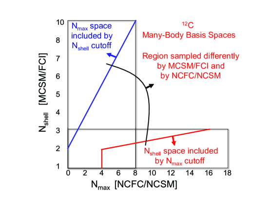
Figure 1: (Color online) Overview of the basis spaces covered with the many-body methods discussed here for the case of ¹²C. $N_{\mathrm{max}}$ is defined as the number of oscillator quanta above lowest possible number of quanta. $N_{\mathrm{shell}}$ is the number of oscillator shells counting the $0s$ shell as the first shell. The MCSM incorporates an FCI space. That is, all single-particle states in the included shells are available to all particles without additional restrictions except for symmetry constraints.

In Fig. 1 we show, for the specific example of ¹²C, how the many-body basis spaces both overlap and differ from each other as a function of increasing cutoff. To indicate an area of complete overlap, the red curve in Fig. 1 borders the $N_{\mathrm{shell}}$ space included as a function of increasing $N_{\mathrm{max}}$. On the other hand, the blue curve borders the region of $N_{\mathrm{max}}$ space included as a function of increasing $N_{\mathrm{shell}}$.

snapshot comparison	FCI	MCSM	NCFC
c.m. motion	approx.	approx.	exact
Spectra	OK	some	OK
wfns $\rightarrow$ observables	✓	✓	✓
Matrix dimension	$\lesssim 10^{10}$	$\lesssim 10^{20}$	$\lesssim 10^{10}$
Scaling with $A$	$A^{18\sim 20}$	$A^{3\sim 5}$	$A^{12\sim 14}$
No. parallel cores	$10^{5}$	$10^{5}$	$10^{5}$
Comp’l bottleneck	Memory	CPU time	Memory

Table 3: Overview of the current features of the three no-core many-body methods employed in this work. The estimates of the scaling with the number of nucleons $A$ are very crude and based on applications to light ($p$-shell) nuclei for a fixed accuracy. The last two lines in the table present overall characteristic features of the codes used for this work.

Table 3 presents a simple set of comparisons and contrasts between the methods. Since $N_{\mathrm{shell}}$ and $N_{\mathrm{max}}$ roughly signify respective accuracies of the methods we hold them fixed to facilitate these comparisons. We emphasize that these are the current features and limitations of these approaches. Additional developments underway are aimed at improving each method, especially the MCSM and NCFC approaches.

The main advantage of the MCSM approach is that, at fixed $N_{\mathrm{shell}}$, the increase in computational needs with increasing nucleon number (“scaling” in Table 3) of the MCSM approach is much slower than that of the FCI appoach. In addition, the increase in computational needs with $A$ of the MCSM approach at fixed $N_{\mathrm{shell}}$ is significantly slower than that of NCFC at fixed $N_{\mathrm{max}}$. Note that the MCSM algorithm is CPU bound, and may be suitable for implementation on general purpose graphical processing units (GPGPUs).

Before progressing to the detailed comparisons among the results from the methods we investigate here, it is worth noting that there are additional efforts aimed at accelerating the convergence of ab initio no-core many-body methods using basis function techniques. The “Importance-Truncated” no-core shell model (IT-NCSM) Roth attempts to estimate the contributions of the many-body configurations above the $N_{\mathrm{max}}$ cutoff using sequences of perturbative contributions to the energy of low-lying states. The symmetry-adapted no-core shell model (SA-NCSM) Dytrych aims to augment the basis space above the $N_{\mathrm{max}}$ cutoff by adding basis states of selected symmetry character that are preferred by low-lying nuclear collective motion. Both methods are producing impressive results. It remains to be seen which method, among the many under investigation, will be more efficient and for which systems and which observables. Outstanding challenges include the fully microscopic description of clustering phenomena and extensions to ab initio nuclear reaction theory.

III Selections of Ingredients

We have outlined above the many-body methods selected for these benchmark comparisons (FCI, MCSM, and NCFC). All results are obtained in a HO basis of single-particle states characterized by the oscillator energy $\hbar\omega$ in MeV and the cutoff of the basis space ($N_{\mathrm{shell}}$ or $N_{\mathrm{max}}$) defined above. We adopt the JISP16 $NN$ interaction Shirokov07 without renormalizing it to a lower momentum scale and we neglect Coulomb and all other interactions. The contributions of spurious c.m. excitation are not discussed here in any detail. Such contributions are absent in conventional NCFC results for ground state observables where we would include the standard Lagrange multiplier term that constrains the c.m. motion to the $0s$ HO state. However, for the present benchmark comparisons, we have dropped the Lagrange multiplier term in the Hamiltonian for simplicity. We do not expect that spurious c.m. effects play a significant role in our benchmark comparisons.

III.1 Interaction

The JISP16 $NN$ interaction is determined by inverse scattering techniques from the $np$ phase shifts and is taken to be charge independent. JISP16 is available in a relative HO basis Shirokov07 and can be written as a sum over partial waves

$$V_{NN}=\sum_{S,{\cal J},T}{\cal P}_{S,{\cal J},T}\sum_{n,\ell,n^{\prime},\ell^{\prime}}\;|n,\ell\rangle\ A^{S,{\cal J},T}_{n\ell,n^{\prime}\ell^{\prime}}\ \langle n^{\prime}\ell^{\prime}|,$$ (5)

where $\hbar\omega=40$ MeV and ${\vec{\cal J}}={\vec{\ell}}+{\vec{s}}$. The HO basis state of relative motion is signified by $|n\ell\rangle$ and the projector onto the specified channel is represented by ${\cal P}_{S,{\cal J},T}$. A small number of coefficients $\{A^{S,{\cal J},T}_{n\ell,n^{\prime}\ell^{\prime}}\}$ are sufficient to describe the phase shifts in each partial wave. Note that the JISP16 interaction is nonlocal and its off-shell properties have been tuned by phase-shift equivalent transformations to produce good properties of light nuclei. For example, JISP16 is tuned in the ${}^{3}S_{1}-^{3}D_{1}$ channel to give a high precision description of the deuteron’s properties. Other channels are tuned to provide good descriptions of ³H binding, the low-lying spectra of ⁶Li and the binding energy of ¹⁶O. With these off-shell tunings to nuclei with $A\geq 3$ one may view JISP16 as simulating, to some approximation, what would appear as $NNN$ interaction contributions (as well as higher-body interactions) in alternative formulations of the nuclear Hamiltonian.

III.2 Nuclear states evaluated

For this benchmark process, we select nine states of light nuclei that includes seven ground states and two excited states; ⁴He ($0^{+}$), ⁶He ($0^{+}$), ⁶Li ($1^{+}$), ⁷Li ($1/2^{-}$, $3/2^{-}$), ⁸Be ($0^{+}$), ¹⁰B ($1^{+}$, $3^{+}$), and ¹²C ($0^{+}$). We compare results for the energy, the point-particle root-mean-square (rms) matter radius, and the electric quadrupole and magnetic dipole moments.

Our goal here is to compare the methods at fixed finite cutoffs. To achieve convergence of the quantities we evaluate will require a much larger effort than the present undertaking. For the benchmark process, we simply proceed through a sequence of cutoffs for each state and each method and obtain results as a function of the oscillator energy, $\hbar\omega$. Then, since all our methods retain the variational principle, we select the optimal $\hbar\omega$ that minimizes the energy for that state and basis space cutoff. We compare the observables for that optimal $\hbar\omega$.

The MCSM results are compared with those of FCI which gives the exact results in the chosen single-particle model space. The FCI results are obtained by the MFDn code Vary92_MFDn ; Maris-ICCS and the MCSM results by the newly developed code ref5 ; Utsuno:2012vm . Note that the FCI results are not available for all the cases presented here due to computational limitations of the FCI approach as indicated by the “Matrix dimension” entry in Table 3.

IV Benchmark Comparisons

IV.1 Results for energies

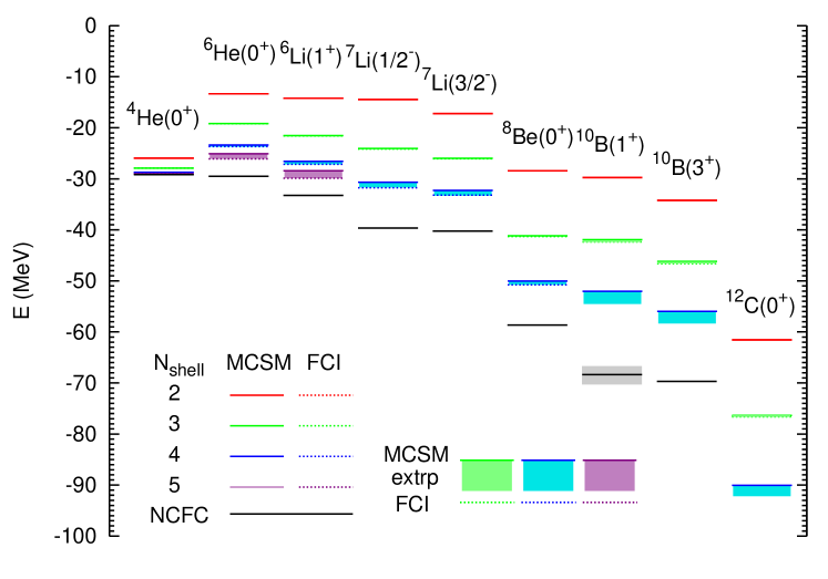
Figure 2: (Color online) Comparisons of the energies between the MCSM and FCI along with the fully converged NCFC results where available. The NCFC result for the ¹⁰B($1^{+}$) state has a large uncertainty indicated by the grey band. The MCSM (FCI) results are shown as the solid (dashed) lines that nearly coincide where both are available. The extrapolated MCSM results are illustrated by bands. From top to bottom, the truncation of the model space is $N_{\mathrm{shell}}=2$ (red), $3$ (green), $4$ (blue), and $5$ (purple). Note that the MCSM results are extrapolated by the energy variance with the second-order polynomials ref6 . Also note that all of the results of ¹⁰B and ¹²C at $N_{\mathrm{shell}}=4$ were obtained only with MCSM.

We present the energies obtained by MCSM and FCI in Fig. 2 through a sequence of $N_{\mathrm{shell}}$ truncations. For the $A=4$ and $6$ systems we obtain results with both MCSM and FCI through $N_{\mathrm{shell}}=5$. For the systems with $A=7$ and $A=8$ we obtain results with both MCSM and FCI through $N_{\mathrm{shell}}=4$. Finally, for ¹⁰B ($1^{+}$, $3^{+}$) and ¹²C ($0^{+}$) we are not able to obtain the FCI results beyond $N_{\mathrm{shell}}=3$ due to computational limitations so the MCSM results at $N_{\mathrm{shell}}=4$ represent predictions. That is, the FCI $M$-scheme matrix dimensions are 18.2 billion and 587 billion as shown in Table 1 for ¹⁰B and ¹²C, respectively, at $N_{\mathrm{shell}}=4$ and these dimensions exceed our current FCI capabilities.

The MCSM and FCI nearly coincide in all cases where both are available. In fact, for $N_{\mathrm{shell}}=2$ they are identical to within machine precision. This can easily be understood because the dimension of the complete FCI basis in the $J$ scheme is below 100 (except for the $J^{\pi}=\frac{3}{2}^{-}$ basis space of ⁷Li, see Table 1), the number of Monte Carlo states used in most of the calculations presented here. Indeed, the MCSM results tend to become independent of the number of Monte Carlo states $N_{b}$ once $N_{b}$ is of the order of 10% to 20% of the dimension $D$ of the underlying FCI basis in the $J$ scheme. Also for $N_{\mathrm{shell}}=3$ the MCSM and FCI results are virtually indistinguishable in Fig. 2. After the extrapolation of the MCSM results using the energy variance ref6 , as discussed below and indicated by shaded regions in Fig. 2, we obtain also very good agreement with the FCI results (where available) for $N_{\mathrm{shell}}\geq 4$.

In Fig. 2 we also present the NCFC results for the energies of the $A=4$ through $10$ nuclei (black solid lines) for comparison. The NCFC results are obtained from calculations up through $N_{\mathrm{max}}=14$ for $A=4$ and $6$, and up through $N_{\mathrm{max}}=12$ for $A=7$ and $8$, using an exponential extrapolation to the infinite basis space. In these cases, the extrapolation uncertainties in the fully converged NCFC results are less than the width of the black line. For $A=10$ we employ results up through $N_{\mathrm{max}}=10$ to obtain the NCFC results. The extrapolation of the $1^{+}$ state in ¹⁰B to obtain the quoted NCFC result has a significantly greater uncertainty due to the occurrence of two close-lying $1^{+}$ states in the calculated spectrum

		$E$ (MeV)
Nuclei	Method	$N_{\mathrm{shell}}=2$	$\hbar\omega$	$D$	$N_{\mathrm{shell}}=3$	$\hbar\omega$	$N_{b}$	$N_{\mathrm{shell}}=4$	$\hbar\omega$	$N_{b}$	$N_{\mathrm{shell}}=5$	$\hbar\omega$	$N_{b}$	NCFC
4He ($0^{+}$)	MCSM	-25.956	30	20	-27.914	30	100	-28.737	30	100	-29.011	25	50	-29.164(2)
	extrp							-28.738(1)			-29.037(1)
	FCI	-25.956			-27.914			-28.738			-29.036
6He ($0^{+}$)	MCSM	-13.343	20	35	-19.186	20	100	-23.480	25	100	-25.080	25	50	-29.51(5)
	extrp				-19.196(1)			-23.687(4)			-26.086(76)
	FCI	-13.343			-19.196			-23.684			-26.079
6Li ($1^{+}$)	MCSM	-14.218	20	97	-21.549	20	100	-26.757	25	100	-28.410	25	50	-33.22(4)
	extrp				-21.581(1)			-27.166(16)			-29.873(83)
	FCI	-14.218			-21.581			-27.168			-29.893
7Li ($1/2^{-}$)	MCSM	-14.459	20	89	-24.073	20	100	-30.904	25	100				-39.8(1)
	extrp				-24.167(2)			-31.780(51)
	FCI	-14.458			-24.165			-31.748
7Li ($3/2^{-}$)	MCSM	-17.232	20	130	-25.978	25	100	-32.494	25	100				-40.4(1)
	extrp				-26.061(4)			-33.272(89)
	FCI	-17.232			-26.063			-33.202
8Be ($0^{+}$)	MCSM	-28.435	20	70	-41.242	25	100	-50.222	25	100				-59.1(1)
	extrp				-41.293(1)			-50.753(32)
	FCI	-28.435			-41.291			-50.756
10B ($1^{+}$)	MCSM	-29.755	25	43	-41.965	25	100	-52.239	25	100				-68.5(1.5)
	extrp				-42.357(46)			-54.89(16)
	FCI	-29.755			-42.338
10B ($3^{+}$)	MCSM	-34.221	25	97	-46.263	25	100	-56.346	25	100				-69.8(2)
	extrp				-46.618(22)			-58.41(13)
	FCI	-34.221			-46.602
12C ($0^{+}$)	MCSM	-62.329	30	20	-76.413	30	100	-90.158	30	100
	extrp				-76.621(4)			-91.957(43)
	FCI	-62.329			-76.621

Table 4: Energies in MeV calculated for the seven ground states and two excited states within the MCSM and FCI methods using the JISP16 $NN$ interaction. The entries of the MCSM indicate the MCSM results before the energy variance extrapolation, while the those of the “extrp” line denote the MCSM results after the extrapolations. The number of Monte Carlo vectors evaluated in the MCSM approach is indicated by $N_{b}$. The value cited for $\hbar\omega$ (units are MeV) represents the value at which the energy for that state reaches its minimum value in that $N_{\mathrm{shell}}$ basis. Uncertainties in extrapolated results are quoted in parenthesis.

In order to stimulate future comparisons with other many body methods, we present detailed results in tables for selected values of $N_{\mathrm{shell}}$. For the energies we present results according to the method and the basis space cutoff in Table 4. All results are presented for the value of $\hbar\omega$ where that state is a minimum in that $N_{\mathrm{shell}}$ basis, except for the NCFC results, which are, within the estimated numerical uncertainty, independent of any basis parameters. Here, we observe that the differences between the MCSM and FCI results is at most a few hundred keV for $N_{\mathrm{shell}}=3$, which is why they are barely distinguishable at the energy scale of Fig. 2. For $N_{\mathrm{shell}}>3$, this difference can be of the order of an MeV or more. However, extrapolated MCSM results agree with the FCI results to within the estimated extrapolation error, with only one case in which the difference is larger than the estimated extrapolation error in Table 4. That case is ⁸Be at $N_{\mathrm{shell}}=4$ where the uncertainty is $1$ keV and the difference is $2$ keV.

The energies converge uniformly from above as expected with increasing $N_{\mathrm{shell}}$. We obtain significant increases in binding with each increment in $N_{\mathrm{shell}}$ and this encourages us to develop the MCSM further in order to access larger $N_{\mathrm{shell}}$ bases. At the present time, our limited results do not indicate a pattern that we can extrapolate to the infinite $N_{\mathrm{shell}}$ limit. However, the expected outcomes of such extrapolations should be the NCFC results shown in Fig. 2 and in the last column of Table 4. Larger $N_{\mathrm{shell}}$ results and extrapolations to the infinite $N_{\mathrm{shell}}$ limit constitute goals for future efforts since our main goal here is to benchmark the MCSM approach through the range of $N_{\mathrm{shell}}$ values accessible by FCI and to compare with the fully converged NCFC where available.

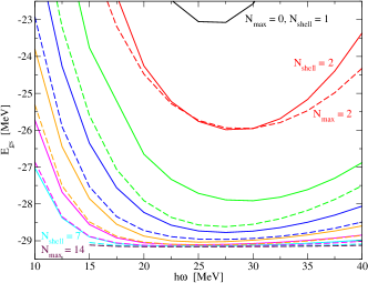
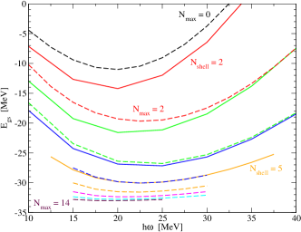
Figure 3: (Color online) Comparisons of the ground state energies of ⁴He (left) and ⁶Li (right) between the FCI with $N_{\mathrm{shell}}$ truncation and NCFC with $N_{\mathrm{max}}$ truncation as a function of the HO frequecy $\hbar\omega$. The FCI (NCFC with cutoff) results are shown as the solid (dashed) lines. From top to bottom, the truncation of the model space increments by unity for $N_{\mathrm{shell}}$ up to $N_{\mathrm{shell}}=7$ (cyan) for ⁴He up to $N_{\mathrm{shell}}=5$ (orange) for ⁶Li, and by two for $N_{\mathrm{max}}$ up to $N_{\mathrm{max}}=14$ (purple) for both ⁴He and ⁶Li.

The detailed convergence pattern for ground state energy for ⁴He is shown for the FCI and NCFC methods in the left panel of Fig. 3 as a function of $\hbar\omega$ and the basis space cutoff ($N_{\mathrm{shell}}$ for FCI; $N_{\mathrm{max}}$ for the approach to NCFC). We define convergence as independence of both $\hbar\omega$ and the basis space cutoff. We note that FCI at $N_{\mathrm{shell}}=8$ and the NCFC truncated at $N_{\mathrm{max}}=10$ both yield almost the same ground state energy of $-29.15$ MeV, even though the dimensions are quite different: the full $N_{\mathrm{shell}}=8$ basis space dimension of ⁴He is $29\ 031\ 044$, whereas the $N_{\mathrm{max}}=10$ basis space dimension is only $196\ 438$, more than two orders of magnitude smaller. The NCFC result for ⁴He is $-29.164(2)$ MeV. For comparison the MCSM results at $N_{\mathrm{shell}}=5$ (the largest MCSM space reported here) and $\hbar\omega=25$ MeV, once extrapolated with the energy-variance method, produces $-29.037(1)$ MeV which agrees to within 1 keV of the FCI result for that space

We also show the detailed convergence patterns for the ground state energy of ⁶Li in the right panel of Fig. 3 for FCI and NCFC at various truncations as a function of $\hbar\omega$ and the basis space cutoff. We note that the convergence trends of the $N_{\mathrm{shell}}=2\rightarrow 5$ results for ⁶Li shown in the right panel of Fig. 3 has both similarities and differences from the pattern for ⁴He seen in the left panel. Both exhibit the “U”-shaped patterns for each truncation with the bottom of the “U” becoming flatter as the cutoff increases. However, for ⁴He, the minimum with respect to $\hbar\omega$ for $N_{\mathrm{shell}}\geq 1$ remains at nearly a constant $\hbar\omega$ value as the cutoff is removed while for ⁶Li that minimum shifts to higher values of $\hbar\omega$.

For ⁶Li, the ground state energy increments by about the same amount from $N_{\mathrm{shell}}=3\rightarrow 4$ as for $N_{\mathrm{shell}}=2\rightarrow 3$. However, there is a significant decrease in the energy increment for the step $N_{\mathrm{shell}}=4\rightarrow 5$. Furthermore, we observe that the energy increment for $N_{\mathrm{shell}}=4\rightarrow 5$ is approximately the difference between the $N_{\mathrm{shell}}=5$ result and the fully converged result given by NCFC. It will be valuable to extend the $N_{\mathrm{shell}}$ cutoff further in a future effort in order to determine the full convergence pattern for ⁶Li. Note that the results obtained in the FCI $N_{\mathrm{shell}}=5$ basis space, with a dimension of 129 million, are very close to the $N_{\mathrm{max}}=6$ results, with a basis space dimension of less than 0.2 million. On the other hand, with only 50 Monte Carlo basis states, the MCSM produces a ground state energy that is within 0.5 MeV of the FCI result at $N_{\mathrm{shell}}=5$. With extrapolation, the ground state energy is within 20 keV of the FCI result with an extrapolation uncertainty of 83 keV.

IV.2 Convergence of MCSM calculations

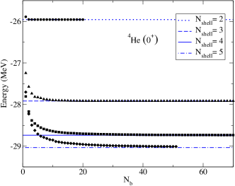
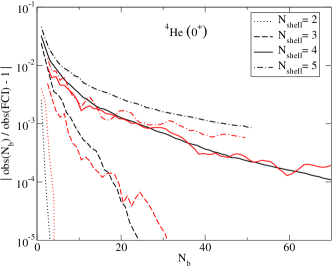
Figure 4: (Color online) The convergence of the MCSM ground state energy of ⁴He to the FCI result for several $N_{\mathrm{shell}}$ values as function of the number of Monte Carlo basis states, $N_{b}$. Top: ground state energy; Bottom: relative difference between MCSM and FCI calculations of the energy (black) and rms matter radius (red).

In top panel of Fig. 4 we show the convergence of the ground state energy of ⁴He as function of the number of the Monte Carlo basis states, $N_{b}$. At every value of $N_{b}$ the MCSM gives a variational upper bound for the energy, and as $N_{b}$ increases, the energy approaches the exact FCI result from above. In the bottom panel we show the relative difference between the MCSM and the FCI result, not only for the energy but also for the rms radius.

Both the ground state energy and the radius of ⁴He converge to within 1% of the exact FCI result with less than ten Monte Carlo basis states, at least up to $N_{\mathrm{shell}}=5$. However, in general, as the number of shells increases, so does the number of Monte Carlo basis states that is needed in order to achieve a fixed level of accuracy: at $N_{\mathrm{shell}}=4$ we need about 20 basis states in order to reach an agreement of 0.1%, but at $N_{\mathrm{shell}}=5$ we need about 50 basis states to reach the same level of accuracy, as can be seen from the bottom panel of Fig. 4.

The number of the Monte Carlo basis states needed for a given level of accuracy depends not only on $N_{\mathrm{shell}}$, but also on the number of nucleons $A$, the quantum numbers of the state under consideration, and the observable, as can be seen from Fig. 5.

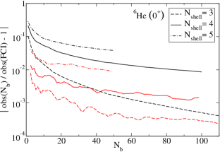
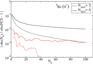
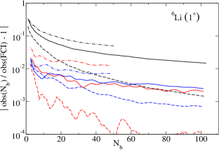
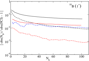
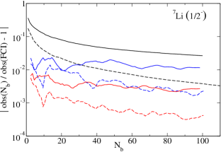
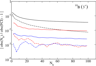
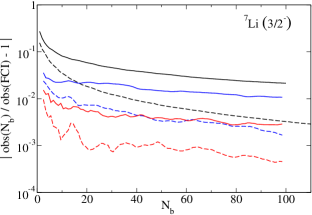
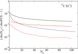
Figure 5: (Color online) The relative difference between MCSM and FCI calculations of the energy (black), rms matter radius (red), and magnetic moment (blue) for several $N_{\mathrm{shell}}$ values as function of the number of MC basis states, $N_{b}$. Top to bottom on the left: ⁶He($J^{\pi}=0^{+}$), ⁶Li($1^{+}$), ⁷Li($\frac{1}{2}^{-}$), and ⁷Li($\frac{3}{2}^{-}$); Top to bottom on the right: ⁸Be($0^{+}$), ¹⁰B($1^{+}$), ¹⁰B($3^{+}$), ¹²C($0^{+}$).

In general, the convergence with $N_{b}$ to the exact FCI result starts out very rapidly, but slows down as $N_{b}$ increases. The energy always converges monotonically (at least for the lowest states of a given spin and parity), because of the variational principle, but other observables such as the rms radii and the magnetic moments do not converge monotonically. On average, however, the difference between the MCSM results and the FCI results decreases with increasing $N_{b}$, as one would expect.

Furthermore, the average convergence rate with increasing $N_{b}$ for different observables of a particular state at fixed $N_{\mathrm{shell}}$ tends to be the same. That is, if the MCSM energy converges rapidly to the FCI energy, then so do the rms radius and magnetic moments of that state, but if the MCSM energy converges slowly, then the other observables converge slowly as well, as one can see from Figs. 4 and 5. This suggests that the wave function obtained with the MCSM converges to the FCI wave function in a systematic manner that can be measured by different observables.

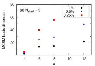
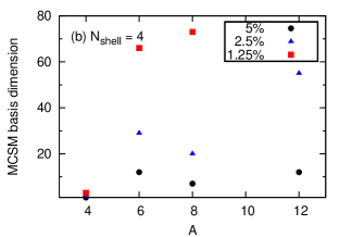
Figure 6: (Color online) Number of MC basis states, $N_{b}$, required for a given accuracy of the MCSM energy for (a) $N_{\mathrm{shell}}=3$ and (b) $N_{\mathrm{shell}}=4$ for ⁴He($J^{\pi}=0^{+}$), ⁶He($0^{+}$), ⁸Be($0^{+}$), and ¹²C($0^{+}$).

In Fig. 6 we show the number of Monte Carlo basis states $N_{b}$ that are needed in order to achieve a specified level of accuracy for the energy as function of $A$ for the four nuclei under consideration that have a $0^{+}$ ground state. Clearly, the convergence for ⁴He is much faster than for any of the other nuclei, and its convergence rate is (unfortunately) not a good indicator for the convergence rate that can be expected for heavier nuclei. For the other three nuclei we see that at $N_{\mathrm{shell}}=3$ a doubling of the MCSM basis dimension leads to a reduction of the difference with the FCI results by (approximately) a factor of two. However, at $N_{\mathrm{shell}}=4$ one needs to more than double the MCSM basis dimension in order to improve the accuracy by a factor of two.

Naively, one might expect that the number of Monte Carlo states needed for a given level of accuracy increases with $A$ (and with $N_{\mathrm{shell}}$) proportional to the dimension of the underlying FCI basis space. However, in practice it turns out that the number of required Monte Carlo states increases much slower with $A$ than the FCI dimension. Note that as $A$ increases, the number of pairwise correlations grows as $A^{2}$ and one might expect to require a similar increase in Monte Carlo basis states in order to achieve a given level of accuracy with strong $NN$ interactions. Hence one could expect a much more modest increase in the number of required Monte Carlo states for a given accuracy than the dramatic growth with $A$ of the dimension of the underlying FCI basis at fixed $N_{\mathrm{shell}}$, see Table 1. Indeed, for $N_{\mathrm{shell}}=3$ this dependence seems to be roughly between linear and quadratic in $A$, though for $N_{\mathrm{shell}}=4$ the trend is not very clear. Also, so far we have only looked at $p$-shell nuclei, and it is as of yet unclear how convergence behaves in the $sd$ shell.

IV.3 Extrapolation to FCI

To obtain the converged energy at fixed $N_{\mathrm{shell}}$ we extrapolate the MCSM results by using the energy variance, which is a new ingredient of the MCSM approach ref6 . The energy variance $\Delta E_{2}$ is defined as

$$\Delta E_{2}=\langle\Psi|H^{2}|\Psi\rangle-\left(\langle\Psi|H|\Psi\rangle\right)^{2}.$$ (6)

For an eigenstate of $H$, the energy variance is zero, but if $\Psi$ is not an exact eigenstate of $H$ the energy variance is larger than zero. As we increase $N_{b}$, the number of Monte Carlo states in the MCSM calculations, we get a better and better approximation of the (lowest) eigenstates of $H$. Therefore, $\Delta E_{2}$ approaches zero from above as $N_{b}$ increases. We use this to obtain an estimate of the exact FCI answer.

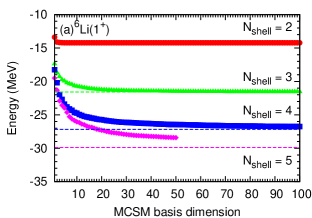
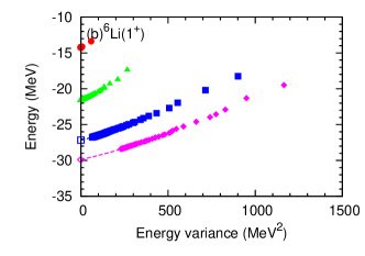
Figure 7: (Color online) The convergence of the MCSM ground state energy of ⁶Li to the FCI result; circles (red), triangles (green), squares (blue), and diamonds (purple) indicate the results at $N_{\mathrm{shell}}=$ $2$, $3$, $4$ and $5$, respectively. (a) Ground state energy as function of the number of Monte Carlo basis states, $N_{b}$; (b) Energy variance $\Delta E_{2}$ and extrapolation to zero energy variance.

We plot the MCSM results for the ground state energy of ⁶Li at different values of $N_{b}$ as a function of the evaluated energy variance $\Delta E_{2}$, see Fig. 7. For $N_{\mathrm{shell}}=2$ and $3$ (red and green symbols), the MCSM energy converges rapidly to the FCI result (top panel), and the energy variance goes to zero (bottom panel). For $N_{\mathrm{shell}}=4$ and $5$ (blue and purple symbols), the energy variance does decrease with increasing $N_{b}$, but does not reach zero in our calculations. For comparison, the open symbols at $\Delta E_{2}=0$ are the results of our (exact) FCI calculations.

The behavior of energy as function of the energy variance is monotonic and can be extrapolated to zero energy variance (which corresponds to the exact energy) by quadratic fitting functions as was done in Ref. ref6 ,

$$E(\Delta E_{2})=c_{0}+c_{1}\Delta E_{2}+c_{2}(\Delta E_{2})^{2}$$ (7)

with the fit parameters, $c_{0}$, $c_{1}$, and $c_{2}$. Here, $c_{0}$ gives the exact energy, $E(\Delta E_{2}=0)$. Indeed, the extrapolations for $N_{\mathrm{shell}}=4$ and $5$ reproduce the exact FCI results to within a few tens of keV, well within the numerical uncertainty in the extrapolation. The numerical uncertainty for the extrapolation is estimated based on the uncertainties $\delta c_{i}$ in each of the three fit parameters $c_{i}$ of the quadratic fit. We treat these three uncertainties as independent, and combine them at the MCSM result with minimum energy variance, $x=\min(\Delta E_{2})$, to produce an overall estimate of the extrapolation uncertainty

$$\delta E=\sqrt{\bigg{(}\frac{\delta E}{\delta c_{0}}\bigg{|}_{x}\,\delta c_{0}\bigg{)}^{2}+\bigg{(}\frac{\delta E}{\delta c_{1}}\bigg{|}_{x}\,\delta c_{1}\bigg{)}^{2}+\bigg{(}\frac{\delta E}{\delta c_{2}}\bigg{|}_{x}\,\delta c_{2}\bigg{)}^{2}}.$$ (8)

The FCI and the MCSM results for the energies with and without the energy variance extrapolation are all summarized in Table 4. Note that we also quote the estimated uncertainty from extrapolation in Table 4.

We use a similar extrapolation for the rms matter radii and, if possible, also for the magnetic dipole and electric quadrupole moments. However, the approach of these observables to the exact FCI result is generally not monotonic, and therefore not as easy to extrapolate. In practice we use a linear extrapolation for these observables, and apply the extrapolation only if the energy variance plot appears to be linear. The detailed dependence of both the energy and the other observables on the energy variance is presented in the Appendix A.

IV.4 Point-particle rms radii

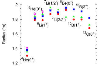
Figure 8: (Color online) Comparisons of the point-particle rms matter radii between the MCSM and FCI. Circles (red), triangles (green), squares (blue) and diamonds (purple) indicate the results at $N_{\mathrm{shell}}=$ $2$, $3$, $4$ and $5$, respectively; solid (open) symbols stand for the MCSM (FCI) results. The MCSM results are those after extrapolation as described in the text. Note that the ¹⁰B and ¹²C results at $N_{\mathrm{shell}}=4$ were obtained only within the MCSM.

		$\sqrt{\langle r^{2}\rangle}$ (fm)
Nuclei	Method	$N_{\mathrm{shell}}=3$	$N_{\mathrm{shell}}=4$	$N_{\mathrm{shell}}=5$
4He ($0^{+}$)	MCSM	1.355	1.379	1.409
	extrp			1.410(1)
	FCI	1.355	1.379	1.410
6He ($0^{+}$)	MCSM	1.843	1.811	1.864
	extrp	1.843(1)	1.813(1)
	FCI	1.843	1.813	1.881
6Li ($1^{+}$)	MCSM	1.871	1.842	1.889
	extrp	1.871(1)	1.846(1)
	FCI	1.871	1.846	1.913
7Li ($1/2^{-}$)	MCSM	1.958	1.921
	extrp	1.959(1)	1.925(1)
	FCI	1.959	1.926
7Li ($3/2^{-}$)	MCSM	1.931	1.895
	extrp	1.932(1)	1.900(1)
	FCI	1.932	1.901
8Be ($0^{+}$)	MCSM	1.831	1.958
	extrp	1.831(1)	1.960(1)
	FCI	1.831	1.960
10B ($1^{+}$)	MCSM	1.834	1.936
	extrp	1.836(1)	1.967(2)
	FCI	1.836
10B ($3^{+}$)	MCSM	1.829	1.909
	extrp	1.830(1)	1.926(1)
	FCI	1.830
12C ($0^{+}$)	MCSM	1.722	1.820
	extrp	1.723(1)	1.833(1)
	FCI	1.723

Table 5: Point-particle rms matter radii (in fm) evaluated relative to the nuclear c.m. The entries labeled “MCSM” indicate the MCSM results before the energy variance extrapolation, while the those of the “extrp” line denote the MCSM results after the extrapolations. See Table 4 for $N_{b}$ and $\hbar\omega$ values.

We present the point-nucleon rms matter radii in Fig. 8 and Table 5 calculated with the wave functions of the MCSM and FCI methods. For this comparison, we evaluate the rms radius of the internal degrees of freedom — that is we use the radius operator that depends only on the coordinates with respect to the c.m. of the system. Thus, although the nuclear wave functions contain mixtures of various components of c.m. motion, the use of the internal coordinates for the radial operator will provide a more accurate rms radius for eventual comparison with experiment. In addition, at the present level of benchmark effort this is sufficient to compare results between these approaches. As mentioned above, the exact separation of the c.m. motion from the internal motion is a nontrivial challenge for the MCSM and FCI approaches while that separation may be assured in the NCFC approach by use of a constraint on the c.m. motion.

The MCSM results in Fig. 8 and those in Table 5 labelled “extrp” are obtained by extrapolation with first-order polynomials using their dependence on the energy variance (see the Appendix for more details). We find the differences between the extrapolated MCSM and FCI rms matter radii to be less than 0.1%, and within the estimate of the extrapolation uncertainty. As a consequence, the open symbols for FCI lie nearly on top of the solid symbols for the extrapolated MCSM so that they are not separately visible in Fig. 8. However, the MCSM results for ⁶He and ⁶Li in $N_{\mathrm{shell}}=5$ with only 50 Monte Carlo basis states are not sufficient for an extrapolation to the exact FCI result; more Monte Carlo states are needed for a reliable extrapolation for these cases. Note that the rms results for ¹⁰B and ¹²C at $N_{\mathrm{shell}}=4$ were obtained only within the MCSM approach.

IV.5 Dipole and quadrupole moments

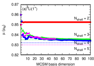
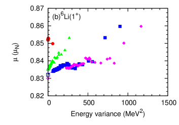
Figure 9: (Color online) The convergence of the MCSM magnetic moment of ⁶Li to the FCI result; circles (red), triangles (green), squares (blue) and diamonds (purple) indicate the results at $N_{\mathrm{shell}}=$ $2$, $3$, $4$ and $5$, respectively. (a) Magnetic moment as function of the number of Monte Carlo basis states, $N_{b}$; (b) Energy variance and extrapolation to zero energy variance. For comparison, the dashed lines (top) and open symbols at $\Delta E_{2}=0$ (bottom) are the results of our (exact) FCI calculations.

In Fig. 9 we plot the MCSM results for the magnetic moment of ⁶Li as function of $N_{b}$ (top) and as function of the evaluated energy variance $\Delta E_{2}$. For $N_{\mathrm{shell}}=2$ and $3$ (red and green symbols), the MCSM results converge rapidly to the FCI result (top panel), and the energy variance goes to zero (bottom panel). For $N_{\mathrm{shell}}=4$ (blue symbols), the MCSM results do seem to converge to the FCI results, and with a linear extrapolation on the energy variance we get good agreement with the FCI results. However, just as for the rms radius, the MCSM results for $\mu$ at $N_{\mathrm{shell}}=5$ with only 50 Monte Carlo basis states are not sufficient for an extrapolation to the exact FCI result; more Monte Carlo states are needed for a reliable extrapolation for this case.

		$\mu$ ($\mu_{N}$)
Nuclei	Method	$N_{\mathrm{shell}}=3$	$N_{\mathrm{shell}}=4$	$N_{\mathrm{shell}}=5$
6Li ($1^{+}$)	MCSM	0.836	0.834	0.836
	extrp	0.835(1)	0.833(1)
	FCI	0.835	0.832	0.830
7Li ($1/2^{-}$)	MCSM	-0.842	-0.816
	extrp	-0.840(1)	-0.806(2)
	FCI	-0.840	-0.807
7Li ($3/2^{-}$)	MCSM	3.061	3.025
	extrp	3.057(1)	2.995(2)
	FCI	3.056	2.993
10B ($1^{+}$)	MCSM	0.503	0.533
	extrp	0.508(1)
	FCI	0.509
10B ($3^{+}$)	MCSM	1.820	1.814
	extrp	1.818(1)	1.819(1)
	FCI	1.818
		$Q$ ($e$fm2)
6Li ($1^{+}$)	MCSM	-0.259	-0.282	-0.276
	extrp	-0.259(1)	-0.285(1)
	FCI	-0.259	-0.285	-0.302
7Li ($3/2^{-}$)	MCSM	-1.766	-2.006
	extrp	-1.750(1)	-1.958(3)
	FCI	-1.750	-1.940
10B ($1^{+}$)	MCSM	-1.712	-2.417
	extrp	-1.703(2)	-2.436(8)
	FCI	-1.698
10B ($3^{+}$)	MCSM	3.532	5.222
	extrp	3.503(1)	5.250(11)
	FCI	3.503

Table 6: Dipole (top) and quadrupole moments (bottom) calculated using the wave functions obtained within the MCSM and FCI methods. The entries of the MCSM indicate the MCSM results before the energy variance extrapolation, while the those of the “extrp” line denote the MCSM results after the extrapolations. See Table 4 for $N_{b}$ and $\hbar\omega$ values.

We summarize our comparison of MCSM and FCI results for the magnetic dipole moments and electric quadrupole moments in Table 6, both with and without the extrapolations of the MCSM results. We use a linear extrapolation using the energy variance, see the Appendix for more details. As mentioned above, we cannot perform a reliable extrapolation from the MCSM results to the exact FCI result for the dipole and quadrupole moments of ⁶Li at $N_{\mathrm{shell}}=5$ with only 50 Monte Carlo states. The only other case for which we could not perform a reliable extrapolation is the magnetic moment of the (lowest) $1^{+}$ state of ¹⁰B. This is likely to be related to the fact that there are two $1^{+}$ states relatively close to each other (experimentally their energies differ by about 1.5 MeV).

We again find the differences between the MCSM and the exact FCI results to be small, typically 1% or less with 100 Monte Carlo states, both for the magnetic dipole moments and for the electric quadrupole moments. The exception is the quadrupole moment of the ground state of ⁶Li: at $N_{\mathrm{shell}}=5$, the difference between the MCSM and FCI calculations is almost 10% with 50 Monte Carlo basis states. Note however that this quadrupole moment is exceptionally small in magnitude: although the relative difference between the NCSM and the FCI result is significantly larger than for most other observables we have looked at, the absolute difference is rather small.

A linear extrapolation using the energy variance brings the MCSM results even closer to the FCI results, see the Appendix for more details. However, the results after 50 Monte Carlo states for ⁶Li at $N_{\mathrm{shell}}=5$ are not sufficiently close to the FCI result to do such an extrapolation.

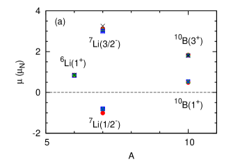
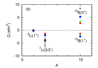
Figure 10: (Color online) Comparisons between the extrapolated MCSM and FCI results for (a) the magnetic dipole moments, and (b) electric quadrupole moments. The conventions for the symbols are same as in Fig. 8; crosses indicate the experimental values for the ground states from Ref. exp_moments .

The magnetic dipole moments, top panel of Fig. 10, depend only very weakly on the basis space truncation parameters $N_{\mathrm{shell}}$ and $\hbar\omega$ — much weaker than the quadrupole moments, bottom panel of Fig. 10, and than the rms radii, Fig. 8. The differences are less than $2\%$ and are not visible on this scale. Furthermore, the dipole moments are in very good agreement with the NCFC results, which means that they are converged to within a few percent with respect to the basis space truncation. Our results with JISP16 are also in good agreement with the available data for the ground states.

On the other hand the quadrupole moments do depend significantly on the basis space truncation parameters $N_{\mathrm{shell}}$ and $\hbar\omega$, as can be seen from the bottom panel of Fig. 10 and from Table 6. This is not surprising, given the dependence of the rms radius on the truncation parameters, and given the fact that the quadrupole moment receives significant contributions from the asymptotic tail of the wave function, which is not very well represented in a HO basis. One needs to include (much) higher HO shells in order to build up a realistic tail for the wave functions. Nevertheless, our results are in qualitative agreement with the available data: small and negative for the ground state of ⁶Li, large and negative for the ground state of ⁷Li, large and positive for the ground state of ¹⁰B.

V Summary and Outlook

We have performed benchmark calculations of the energies, point-particle rms matter radii, and electromagnetic moments for nine states in light nuclei ranging from ⁴He to ¹²C. Where possible, we have solved for these properties using the FCI, MCSM and NCFC approaches. The energies and the point-particle rms matter radii calculated by MCSM were extrapolated as a function of energy variance. All results are found to be consistent with each other to within quoted uncertainties when they could be quantified. Where we could not obtain quantified uncertainties, the results were found to differ typically by a few percent among the available methods with very few exceptions. The MCSM and FCI results are very close to each other with small differences (of a few percent in most cases) arising mainly from the limited number of MCSM basis sampled stochastically for diagonalization and from MCSM energy variance extrapolation uncertainties. We include selected NCFC results in order to gauge the increases in basis spaces needed to better approach the fully converged results (basis space cutoff independence) in future efforts.

Since the MCSM computational effort scales more favorably with increasing basis space and increasing nucleon number, we expect that the MCSM will further develop into a powerful tool for ab initio nuclear theory. To reach this goal, we will need to expand the basis space, treat the role of c.m. motion and include the Coulomb interaction as well as $NNN$ interactions. These challenges will be addressed in future efforts.

*

Appendix A Extrapolation of MCSM results

With increasing Monte Carlo basis dimension $N_{b}$, the MCSM results converge to the FCI results. In order to obtain an estimate of that exact FCI answer, we extrapolate the energy and other observables evaluated by MCSM using the energy variance. That is, the MCSM results are plotted as a function of the evaluated energy variance

$$\Delta E_{2}=\langle\Psi|H^{2}|\Psi\rangle-\left(\langle\Psi|H|\Psi\rangle\right)^{2}$$ (9)

and then extrapolated to zero variance as we show below. We also investigate the uncertainties of this extrapolation and report those uncertainties in Tables 4–6.

Figure 11 shows the energies as function of the energy variance for ⁶He, ⁶Li, ⁷Li, ⁸Be, ¹⁰B, and ¹²C. For $N_{\mathrm{shell}}=2$ and $3$ there is no need for any extrapolation: with 100 Monte Carlo states, there is very good agreement between the MCSM results and the FCI results. For $N_{\mathrm{shell}}=4$ and $5$ we use a quadratic polynomial fit to extrapolate $\Delta E_{2}$ to zero. We also make an estimate of the numerical uncertainty in this extrapolation. These extrapolated MCSM results are in good agreement with the available FCI results (indicated by the open symbols at $\Delta E_{2}=0$). In Table 4 we give both the MCSM results, and the extrapolated results with extrapolation uncertainty.

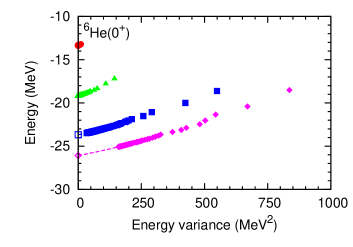
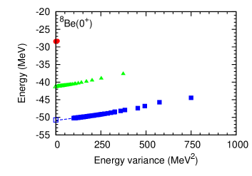
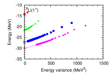
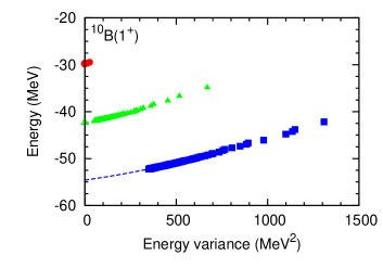
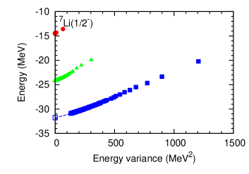
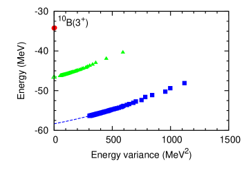
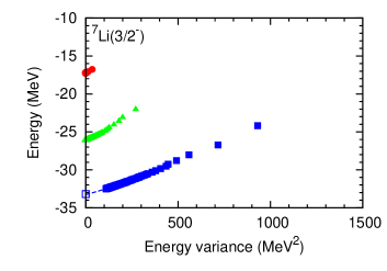
Figure 11: (Color online) The energy variance and extrapolation to the FCI result for the energies. Circles (red), triangles (green), squares (blue) and diamonds (purple) indicate the results at $N_{\mathrm{shell}}=2$, $3$, $4$ and $5$, respectively; the open symbols at $\Delta E_{2}=0$ are the exact FCI energies. Top to bottom on the left: ⁶He($J^{\pi}=0^{+}$), ⁶Li($1^{+}$), ⁷Li($\frac{1}{2}^{-}$), and ⁷Li($\frac{3}{2}^{-}$); Top to bottom on the right: ⁸Be($0^{+}$), ¹⁰B($1^{+}$), ¹⁰B($3^{+}$), and ¹²C($0^{+}$).

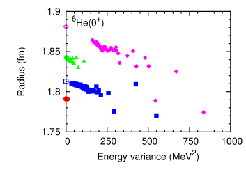
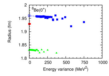
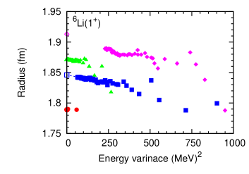
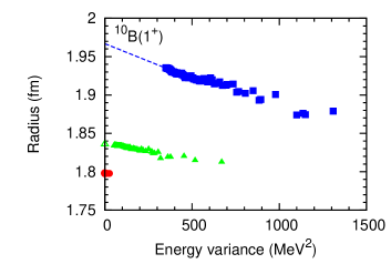
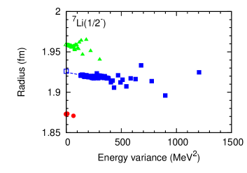
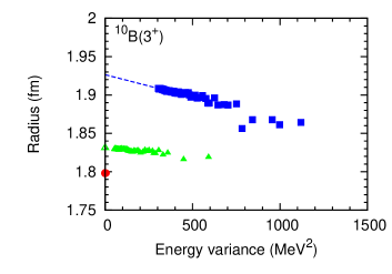
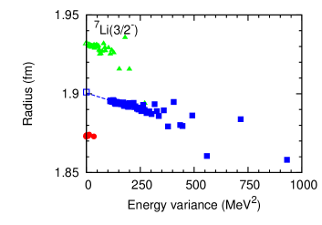
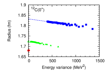
Figure 12: (Color online) The energy variance and extrapolation to the FCI result for the rms radii. Symbols are the same as in Fig. 11. Top to bottom on the left: ⁶He($J^{\pi}=0^{+}$), ⁶Li($1^{+}$), ⁷Li($\frac{1}{2}^{-}$), and ⁷Li($\frac{3}{2}^{-}$); Top to bottom on the right: ⁸Be($0^{+}$), ¹⁰B($1^{+}$), ¹⁰B($3^{+}$), and ¹²C($0^{+}$).

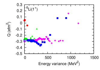
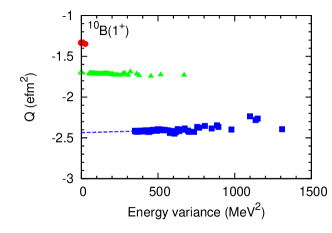
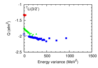
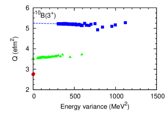
Figure 13: (Color online) The energy variance and extrapolation to the FCI result for the quadrupole moments. Symbols are the same as in Fig. 11. Top and bottom on the left: ⁶Li($1^{+}$) and ⁷Li($\frac{3}{2}^{-}$); Top and bottom on the right: ¹⁰B($1^{+}$) and ¹⁰B($3^{+}$).

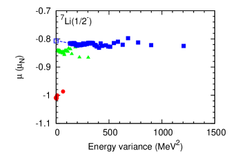
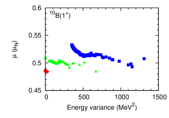
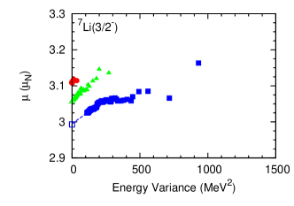
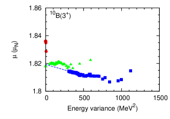
Figure 14: (Color online) The energy variance and extrapolation to the FCI result for the dipole moments. Symbols are the same as in Fig. 11. Top and bottom on the left: ⁷Li($\frac{1}{2}^{-}$) and ⁷Li($\frac{3}{2}^{-}$); Top and bottom on the right: ¹⁰B($1^{+}$) and ¹⁰B($3^{+}$).

Figure 12 shows the rms matter radii as function of the energy variance for ⁶He, ⁶Li, ⁷Li, ⁸Be, ¹⁰B, and ¹²C. For $N_{\mathrm{shell}}=2$ and $3$ there is no need for any extrapolation: with 100 Monte Carlo states, there is very good agreement between the MCSM results and the FCI results. For $N_{\mathrm{shell}}=4$ we use a linear fit to extrapolate $\Delta E_{2}$ to zero. We also make an estimate of the numerical uncertainty in this extrapolation. These extrapolated MCSM results are in good agreement with the available FCI results (indicated by the open symbols at $\Delta E_{2}=0$). In Table 5 we give both the MCSM results, and the extrapolated results with extrapolation uncertainty.

Unfortunately, 50 Monte Carlo states is not sufficient to extrapolate the radii of ⁶Li and ⁶He at $N_{\mathrm{shell}}=5$: the purple diamonds in the upper left figures cannot be extrapolated reliably to $\Delta E_{2}=0$. This is also the case for the magnetic dipole moment, see Fig. 10, and the electric quadrupole moment, see Fig. 13 below.

Figure 13 shows the electric quadrupole moments as function of the energy variance for the states that have $J\geq 1$. For $N_{\mathrm{shell}}=2$ there is no need for any extrapolation. However, both the $N_{\mathrm{shell}}=3$ and the $N_{\mathrm{shell}}=4$ MCSM results with 100 Monte Carlo states can be improved by a linear extrapolation. As already mentioned, 50 Monte Carlo states is not sufficient to extrapolate the quadrupole moment of ⁶Li at $N_{\mathrm{shell}}=5$.

Finally, in Fig. 14 we show the magnetic dipole moments as function of the energy variance for the ⁷Li and ¹⁰B states that have $J\geq 1$. Again, for $N_{\mathrm{shell}}=2$ there is no need for any extrapolation. Both the $N_{\mathrm{shell}}=3$ and the $N_{\mathrm{shell}}=4$ MCSM results with 100 Monte Carlo states can be improved by a linear extrapolation. However, the dependence of the magnetic moment of the (lowest) $1^{+}$ state of ¹⁰B does not seem to converge as the energy variance decreases. This is possibly caused by the proximity of a second $1^{+}$.

The extrapolated MCSM results for both the magnetic moments and the quadrupole moments are in good agreement with the available FCI results (indicated by the open symbols at $\Delta E_{2}=0$). In Table 6 we give both the MCSM results, and the extrapolated results with extrapolation uncertainty.

References

- (1) S. C. Pieper, R. B. Wiringa, and J. Carlson, Phys. Rev. C 70, 054325 (2004); K. M. Nollett, S. C. Pieper, R. B. Wiringa, J. Carlson, and G. M. Hale Phys. Rev. Lett. 99, 022502 (2007); S. C. Pieper, in Proceedings of the International School of Physics “Enrico Fermi”, Course CLXIX, edited by A. Covello, F. Iachello and R. A. Ricci (Societ Italiana di Fisica, Bologna, 2008), p. 111, arXiv:0711.1500 [nucl-th]; reprinted in La Rivista del Nuovo Cimento, 31, 709, (2008), and references therein.
- (2) P. Navrátil, J. P. Vary, and B. R. Barrett, Phys. Rev. Lett. 84, 5728 (2000); Phys. Rev. C 62, 054311 (2000); S. Quaglioni and P. Navrátil, Phys. Rev. Lett. 101, 092501 (2008); Phys. Rev. C 79, 044606 (2009).
- (3) G. Hagen, T. Papenbrock and M. Hjorth-Jensen, Phys. Rev. Lett. 104 182501(2010), and references therein.
- (4) E. Epelbaum, W. Glöckle, and Ulf-G. Meissner, Nucl. Phys. A 637, 107 (1998); 671, 295 (2000).
- (5) D. R. Entem and R. Machleidt, Phys. Rev. C 68, 041001(R) (2003).
- (6) R. B. Wiringa, V. G. J. Stoks and R. Schiavilla, Phys. Rev. C 51, 38 (1995).
- (7) S. C. Pieper, V. R. Pandharipande, R. B. Wiringa, and J. Carlson, Phys. Rev. C 64, 014001 (2001)
- (8) S. C. Pieper, AIP Conf. Proc. No. 1011, 143(2008).
- (9) A. M. Shirokov, J. P. Vary, A. I. Mazur and T. A. Weber, Phys. Letts. B 644, 33 (2007); A. M. Shirokov, J. P. Vary, A. I. Mazur, S. A. Zaytsev and T. A. Weber, ibid. 621, 96 (2005); subroutines to generate this interaction in the relative-center-of-mass HO basis are available at nuclear.physics.iastate.edu.
- (10) M. Honma, T. Mizusaki and T. Otsuka, Phys. Rev. Lett. 75, 1284 (1995); 77, 3315 (1996); T. Otsuka, M. Honma and T. Mizusaki, ibid. 81, 1588 (1998); for review and further references, see T. Otsuka, M. Honma, T. Mizusaki, N. Shimizu, and Y. Utsuno, Prog. Part. Nucl. Phys. 47, 319 (2001).
- (11) P. Maris, J. P. Vary, A. M. Shirokov, Phys. Rev. C 79, 014308 (2009); P. Maris, A. M. Shirokov and J. P. Vary, ibid. 81, 021301(R) (2010); C. Cockrell, J. P. Vary and P. Maris, ibid. 86, 034325 (2012).
- (12) G. Hagen, T. Papenbrock and D. J. Dean, Phys. Rev. Lett. 103, 062503 (2009).
- (13) J. P. Vary, The Many Fermion Dynamics Shell Model Code, Iowa State University, 1992 (unpublished); J. P. Vary and D. C. Zheng, ibid., 1994 (unpublished); P. Sternberg, E. G. Ng, C. Yang, P. Maris, J. P. Vary, M. Sosonkina, and H. V. Le, in Proceedings of the 2008 ACM/IEEE conference on Supercomputing (IEEE Press, Piscataway, NJ, 2008), pp. 15:1–15:12.
- (14) P. Maris, M. Sosonkina, J. P. Vary, E. G. Ng and C. Yang, International Conference on Computer Science, ICCS 2010, Procedia Computer Science 1, 97 (2010).
- (15) N. Shimizu, Y. Utsuno, T. Abe, and T. Otsuka, RIKEN Accel. Prog. Rep. 43, 46 (2010).
- (16) Y. Utsuno, N. Shimizu, T. Otsuka and T. Abe, Comput. Phys. Comm. 184, 102 (2013).
- (17) N. Shimizu, Y. Utsuno, T. Mizusaki, T. Otsuka, T. Abe, and M. Honma, Phys. Rev. C82, 061305(R) (2010); AIP Conf. Proc. No. 1355, 138 (2011).
- (18) T. Abe, P. Maris, T. Otsuka, N. Shimizu, Y. Utsuno, and J. P. Vary, AIP Conf. Proc. 1355, 173 (2011).
- (19) G. Puddu, arXiv:1201.0600 [nucl-th].
- (20) R. Roth, Phys. Rev. C 79, 064324 (2009).
- (21) T. Dytrych, K. D. Sviratcheva, C. Bahri, J. P. Draayer and J. P. Vary, Phys. Rev. Lett. 98, 162503 (2007); T. Dytrych, K. D. Sviratcheva, C. Bahri, J. P. Draayer and J. P. Vary, J. Phys. G. 35, 095101 (2008); ibid. 35, 123101 (2008).
- (22) L. Liu, T. Otsuka, N. Shimizu, Y. Utsuno and R. Roth, Phys. Rev. C 86, 014302 (2012).
- (23) N. J. Stone, Atomic Data and Nuclear Data Tables 90, 75 (2005).