Automated Feedback Generation for Introductory Programming Assignments

Abstract

We present a new method for automatically providing feedback for introductory programming problems. In order to use this method, we need a reference implementation of the assignment, and an error model consisting of potential corrections to errors that students might make. Using this information, the system automatically derives minimal corrections to student’s incorrect solutions, providing them with a quantifiable measure of exactly how incorrect a given solution was, as well as feedback about what they did wrong.

We introduce a simple language for describing error models in terms of correction rules, and formally define a rule-directed translation strategy that reduces the problem of finding minimal corrections in an incorrect program to the problem of synthesizing a correct program from a sketch. We have evaluated our system on thousands of real student attempts obtained from 6.00 and 6.00x. Our results show that relatively simple error models can correct on average $65\%$ of all incorrect submissions.

1 Introduction

There has been a lot of interest recently in making quality education more accessible to students worldwide using information technology. Several education initiatives such as EdX, Coursera, and Udacity are teaming up with experts to provide online courses on various college-level subjects ranging from computer science to physics and psychology. These courses, also called massive open online courses (MOOC), are typically taken by several thousands of students worldwide, and presents many interesting challenges that are not present in a traditional classroom setting consisting of only a few hundred students. One such challenge in these courses is to provide personalized feedback on practice exercises and assignments to a large number of students. We consider the problem of providing automated feedback for online introductory programming courses in this paper. We envision this technology to be useful in a traditional classroom setting as well.

The two most commonly used methods today for providing feedback on programming problems are: (i) test-cases based feedback and (ii) peer-feedback Ertmer et al. [2007]. In automated test-cases based feedback, the student program is run on a set of test cases and the failing test cases are reported back as feedback to the student. This is also how the 6.00x course (Introduction to Computer Science and Programming) offered by MITx currently provides feedback for the python programming exercises. The provided feedback of failing test cases is however not ideal, especially for beginner programmers, as they find it difficult to map the failing test cases to errors in their code. We found a lot of students posting their submissions on the discussion board seeking help from instructors and other students after struggling for several hours to correct the mistakes themselves. In fact, for the classroom version of the Introduction to Programming course (6.00) taught at MIT, the teaching assistants are required to manually go through each student submission and provide qualitative feedback describing exactly what is wrong with the submission and how to correct it. This manual feedback by teaching assistants is simply prohibitive for the number of students in the online class setting.

The second approach of peer-feedback is being suggested as a potential solution to this problem. In this approach, the peer students who are also taking the same course answer the posts on the discussion boards – this way the problem of providing feedback is distributed across several peer students. Unfortunately, providing quality feedback is a big challenge for experienced teaching assistants, and therefore it presents an even bigger challenge for the peer students who are also beginning to learn programming themselves. From the 6.00x discussion boards, we observed that in many instances students had to wait several hours (or days) to get any feedback, and in many cases the feedback provided was either too general, incomplete or even wrong in a few cases.

In this paper, we present an automated technique to provide feedback for introductory programming assignments. The approach leverages program synthesis technology to automatically determine minimal fixes to the student’s solution that will make it match the behavior of a reference solution written by the instructor. This technology makes it possible to provide students with precise feedback about what they did wrong and how to correct them. The problem of providing automatic feedback appears to be related to the problem of automated bug fixing, but it differs from it in following two significant respects:

• The complete specification is known. An important challenge in automatic debugging is that there is no way to know whether a fix is addressing the root cause of a problem, or simply masking it and potentially introducing new errors. Usually the best one can do is check a candidate fix against a test suite or a partial specification Forrest et al. [2009]. While providing feedback on the other hand, the solution to the problem is known, and it is safe to assume that the instructor already wrote a correct reference implementation for the problem.

• Errors are predictable. In a homework assignment, everyone is solving the same problem after having attended the same lectures, so errors tend to follow predictable patterns. This makes it possible to use a model-based feedback approach, where the potential fixes are guided by a model of the kinds of errors students typically make for a given problem.

These simplifying assumptions, however, introduce their own set of challenges. For example, since the complete specification is known, the tool now needs to reason about the equivalence of the student solution with the reference implementation. Also, in order to take advantage of the predictability of errors, the tool needs to be parameterized with models that describe the classes of errors. And finally, these programs can be expected to have higher density of errors than production code, so techniques like the one suggested by Jose and Majumdar [2011], which attempts to correct bugs one path at a time will not work for many of these problems that require coordinated fixes in multiple places.

Our automated feedback generation technique handles all of these challenges. The tool can reason about the semantic equivalence of student programs and reference implementations written in a fairly large subset of python, so the instructor does not have to learn a new formalism to write specifications. The tool also provides an error model language that can be used to write an error model: a very high level description of potential corrections to errors that students might make in the solution. When the system encounters an incorrect solution by a student, it symbolically explores the space of all possible combinations of corrections allowed by the error model and finds a correct solution requiring a minimal set of corrections.

We have evaluated our approach on thousands of student solutions on programming problems obtained from the 6.00x submissions and discussion boards, and from the 6.00 class submissions. These problems constitute a major portion of first month of assignment problems. Our tool can successfully provide feedback on over $65\%$ of the incorrect solutions.

This paper makes the following key contributions:

• We show that the problem of providing automated feedback for introductory programming assignments can be framed as a synthesis problem. Our reduction uses a constraint-based mechanism to model python’s dynamic typing and supports complex python constructs such as closures, higher-order functions and list comprehensions.

• We define a high-level language Eml that can be used to provide correction rules to be used for providing feedback. We also show that a small set of such rules is sufficient to correct thousands of incorrect solutions written by students.

• We report the successful evaluation of our technique on thousands of real student attempts obtained from 6.00 and 6.00x classes, as well as from Pex4Fun website. Our tool can provide feedback on 65% of all submitted solutions that are incorrect in about $10$ seconds on average.

2 Overview of the approach

In order to illustrate the key ideas behind our approach, consider the problem of computing the derivative of a polynomial whose coefficients are represented as a list of integers. This problem is taken from week 3 problem set of 6.00x (PS3: Derivatives). Given the input list poly, the problem asks students to write the function computeDeriv that computes a list poly’ such that

$$\texttt{poly'}=\left\{\begin{array}[]{cl}\{\texttt{i}\times\texttt{poly[i]}\;|\;0<\texttt{i}<\texttt{len(poly)}\}&\mbox{if {len(poly)} > 1}\\ [0.0]&\mbox{if {len(poly)} = 1}\end{array}\right.$$

For example, if the input list poly is $[2,-3,1,4]$ (denoting $f(x)=4x^{3}+x^{2}-3x+2$), the computeDeriv function should return $[-3,2,12]$ (denoting the derivative $f^{\prime}(x)=12x^{2}+2x-3$). The reference implementation for the computeDeriv function is shown in Figure 1. This problem teaches concepts of conditionals and iteration over lists. For this problem, students struggled with many low-level python semantics issues such as the list indexing and iteration bounds. In addition, they also struggled with conceptual issues such as missing the corner case of handling lists consisting of single element (denoting constant function).

⬇

1def computeDeriv_list_int(poly_list_int):

2 result = []

3 for i in range(len(poly_list_int)):

4 result += [i * poly_list_int[i]]

5 if len(poly_list_int) == 1:

6 return result # return [0]

7 else:

8 return result[1:] # remove the leading 0

Figure 1: The reference implementation for computeDeriv function.

⬇ 1def computeDeriv(poly): 2 deriv = [] 3 zero = 0 4 if (len(poly) == 1): 5 return deriv 6 for expo in range (0, len(poly)): 7 if (poly[expo] == 0): 8 zero += 1 9 else: 10 deriv.append(poly[expo]*expo) 11 return deriv	The program requires 3 changes: • In the return statement return deriv in line 5, replace deriv by [0]. • In the comparison expression (poly[expo] == 0) in line 7, change (poly[expo] == 0) to False. • In the expression range(0, len(poly)) in line 6, increment 0 by 1.
(a) Student’s solution	(b) Generated Feedback

Figure 2: (a) A student’s computeDeriv solution from the 6.00x discussion board and (b) the feedback generated by our tool on this solution.

A student solution for the computeDeriv problem taken from the 6.00x discussion forum is shown in Figure 2(a). The student posted the code in the forum seeking help and received two responses. The first response asked the student to look for the first if-block return value, and the second response said that the code should return $[0]$ instead of empty list for the first if statement. There are many different ways to modify the code to return $[0]$ for the case len(poly)=1. The student chose to change the initialization of the deriv variable from $[~{}]$ to the list $[0]$. The problem with this modification is that the result will now have an additional $0$ in front of the output list for all input lists (which is undesirable for lists of length greater than $1$). The student then posted the query again on the forum on how to remove the leading $0$ from result, but unfortunately this time did not get any more response.

Our tool generates the feedback shown in Figure 2(b) for the student program in about $40$ seconds. During these $40$ seconds, the tool searches over more than $10^{7}$ candidate fixes and finds the fix that requires minimum number of corrections. There are three problems with the student code: first it should return $[0]$ in line $5$ as was suggested in the forum but wasn’t specified how to make the change, second the if block should be removed in line $7$, and third that the loop iteration should start from index $1$ instead of $0$ in line $6$. The generated feedback consists of four pieces of information (shown in bold in the figure for emphasis):

• the location of the error denoted by the line number.

• the problematic expression in the line.

• the sub-expression which needs to be modified.

• the new modified value of the sub-expression.

The feedback generator is parameterized with a feedback-level parameter to generate feedback consisting of different combinations of the four information depending on how much information the instructor is willing to provide to the student.

2.1 Workflow

In order to provide the level of feedback described above, the tool needs some information from the instructor. First, the tool needs to know what the problem is that the students are supposed to solve. The instructor provides this information by writing a reference implementation such as the one in Figure 1. Since python is dynamically typed, the instructor also provides the types of function arguments and return value. In Figure 1, the instructor specifies the type of input argument to be list of integers (poly_list_int) by appending the type to the name.

In addition to the reference implementation, the tool needs a description of the kinds of errors students might make. We have designed an error model language Eml, which can describe a set of correction rules that denote the potential corrections to errors that students might make. For example, in the student attempt in Figure 2(a), we observe that corrections often involve modifying the return value and the range iteration values. We can specify this information with the following three correction rules:

$$\texttt{return}~{}a \rightarrow \texttt{return}~{}[0]$$

$$\texttt{range}(a_{1},a_{2}) \rightarrow \texttt{range}(a_{1}+1,a_{2})$$

$$a_{0}==a_{1} \rightarrow$$ False

The correction rule $\texttt{return}~{}a\rightarrow\texttt{return}~{}[0]$ states that the expression of a return statement can be optionally replaced by $[0]$. The error model for this problem that we use for our experiments is shown in Figure 8, but we will use this simple error model for simplifying the presentation in this section. In later experiments, we also show how only a few tens of incorrect solutions can provide enough information to create an error model that can automatically provide feedback for thousands of incorrect solutions.

The tool now needs to explore the space of all candidate programs based on applying these correction rules to the student program, and compute the candidate program that is equivalent to the reference implementation and that requires minimum number of corrections. We use constraint-based synthesis technology Solar-Lezama [2008]; Gulwani et al. [2008]; Srivastava et al. [2010] to efficiently search over this large space of programs. Specifically, we use the Sketch synthesizer that uses a sat-based algorithm to complete program sketches (programs with holes) so that they meet a given specification. We extend the Sketch synthesizer with support for minimize hole expressions whose values are computed efficiently by using incremental constraint solving. To simplify the presentation, we use a simpler language mPy (miniPython) in place of python to explain the details of our algorithm. In practice, our tool supports a fairly large subset of python including closures, higher order functions and list comprehensions.

2.2 Solution Strategy

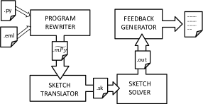
Figure 3: The architecture of our automated feedback generation tool.

The architecture of our tool is shown in Figure 3. The solution strategy to find minimal corrections to a student’s solution is based on a two-phase translation to the Sketch synthesis language. In the first phase, the Program Rewriter uses the correction rules to translate the solution into a language we call $\widetilde{\textsc{mPy}}$; this language provides us with a concise notation to describe sets of mPy candidate programs, together with a cost model to reflect the number of corrections associated with each program in this set. In the second phase, this $\widetilde{\textsc{mPy}}$ program is translated into a sketch program by the Sketch Translator.

In the case of example in Figure 2(a), the Program Rewriter produces the $\widetilde{\textsc{mPy}}$ program shown in Figure 4 using the correction rules from Section 2.1. This program includes all the possible corrections induced by the correction rules in the model. The $\widetilde{\textsc{mPy}}$ language extends the imperative language mPy with expression choices, where the choices are denoted with squiggly brackets. Whenever there are multiple choices for an expression or a statement, the zero-cost choice, the one that will leave the expression unchanged, is boxed. For example, the expression choice $\{\framebox{$a_{0}$},a_{1},\cdots,a_{n}\}$ denotes a choice between expressions $a_{0}$, $\cdots$, $a_{n}$ where $a_{0}$ denotes the zero-cost default choice.

⬇

1def computeDeriv(poly):

2 deriv = []

3 zero = 0

4 if ({len(poly) == 1, False}):

5 return {deriv,[0]}

6 for expo in range ({0,1}, len(poly)):

7 if ({poly[expo] == 0,False}):

8 zero += 1

9 else:

10 deriv.append(poly[expo]*expo)

11 return {deriv,[0]}

Figure 4: The resulting $\widetilde{\textsc{mPy}}$ program after applying correction rules to program in Figure 2(a).

For this simple program, the three correction rules induce a space of $32$ different candidate programs. This candidate space is fairly small, but the number of candidate programs grow exponentially with the number of correction places in the program and with the number of correction choices in the rules. The error model that we use in our experiments induces a space of more than $10^{12}$ candidate programs for some of the benchmark problems. In order to search this large space efficiently, the program is translated to a sketch by the Sketch Translator.

2.3 Synthesizing Corrections with Sketch

The Sketch Solar-Lezama [2008] synthesis system allows programmers to write programs while leaving fragments of it unspecified as holes; the contents of these holes are filled up automatically by the synthesizer such that the program conforms to a specification provided in terms of a reference implementation. The synthesizer uses the CEGIS algorithm Solar-Lezama et al. [2005] to efficiently compute the values for holes and uses bounded symbolic verification techniques for performing equivalence check of the two implementations.

There are two key aspects in the translation of an $\widetilde{\textsc{mPy}}$ program to a Sketch program. The first aspect is specific to the python language. Sketch supports high-level features such as closures and higher-order functions which simplifies the translation, but it is statically typed whereas mPy programs (like python) are dynamically typed. The translation models the dynamically typed variables and operations over them using struct types in Sketch in a way similar to the union types. The second aspect of the translation is the modeling of set-expressions in $\widetilde{\textsc{mPy}}$ using ?? (holes) in Sketch, which is language independent.

⬇ struct MultiType{ int val, type; MTList lst; }

⬇ struct MTList{ int len; MultiType[len] lVals; }

Figure 5: The definition of MultiType struct for encoding dynamic types in python.

The dynamic variable types in mPy language are modeled using the MultiType struct defined in Figure 5. The MultiType struct consists of a type field that denotes the dynamic type of variables and currently supports the following set of types {INTEGER, BOOL, TYPE, LIST, TUPLE}. The val field stores the integer value or the Boolean value of the variables, whereas the lst field of type MTList stores the value of list and tuple variables. The MTList struct consists of a field len that denotes the length of the list and a field lVals of type array of MultiType that stores the list elements. For example, the integer value 5 is represented as the value MultiType(val=5, flag=INTEGER) and the list [1,2] is represented as the value MultiType(lst=new MTList(len=2,lVals={new MultiType(val=1,flag=INTEGER), new MultiType(val=2,flag=INTEGER)}), flag=LIST).

The second key aspect of this translation is the translation of expression choices in $\widetilde{\textsc{mPy}}$. The Sketch construct ?? denotes an unknown integer hole that can be assigned any constant integer value by the synthesizer. The expression choices in $\widetilde{\textsc{mPy}}$ are translated to functions in Sketch that based on the unknown hole values return either the default expression or one of the other expression choices. Each such function is associated with a unique Boolean choice variable, which is set by the function whenever it returns a non-default expression choice. For example, the set-statement return {deriv,[0]}; (line $5$ in Figure 4) is translated to return modRetVal0(deriv), where the modRetVal0 function is defined as:

⬇

MultiType modRetVal0(MultiType a){

if(??) return a; // default choice

choiceRetVal0 = True; // non-default choice

MTList list = new MTList(lVals={new MultiType(val=0, flag=INTEGER)}, len=1);

return new MultiType(lst=list, type = LIST);

}

The translation phase also generate a Sketch harness that calls and compares the outputs of the translated student and reference implementations on all inputs of a bounded size. For example in case of the computeDeriv function that takes a list as input, with bounds of $n=4$ for both the number of integer bits and the maximum length of the input list, the harness makes sure that the output of the two implementations match for more than $2^{16}$ different inputs as opposed to $10$ test-cases used in 6.00x. The harness also defines a totalCost variable as a function of all choice variables that computes the total number of modifications performed in the original program, and asserts that the value of totalCost should be minimized. The synthesizer then solves this minimization problem efficiently using an incremental solving algorithm CEGISMIN described in Section 4.2.

After the synthesizer finds a solution, the Feedback Generator uses the solution to the unknown integer holes in the sketch to compute the choices made by the synthesizer and generates the corresponding feedback. For this example, the tool generates the feedback shown in Figure 2(b) in less than $40$ seconds.

3 Eml: Error Model Language

In this section, we describe the syntax and semantics of the error model language Eml. An Eml error model consists of a set of rewrite rules that captures the potential corrections for mistakes that students might make in their solutions. We define the rewrite rules over a simple python-like imperative language mPy. A rewrite rule transforms a program element in mPy to a set of weighted mPy program elements. This weighted set of mPy program elements is represented succinctly as an $\widetilde{\textsc{mPy}}$ program element, where $\widetilde{\textsc{mPy}}$ extends the mPy language with set-exprs (set of expressions) and set-stmts (set of statements). The weight associated with a program element in this set denotes the cost of performing the corresponding correction. An error model transforms an mPy program to an $\widetilde{\textsc{mPy}}$ program (representing a set of mPy programs) by recursively applying the rewrite rules. We show that this transformation is deterministic and is guaranteed to terminate on well-formed error models.

3.1 mPy and $\widetilde{\textsc{mPy}}$ languages

$\displaystyle\mbox{Arith Expr }a$ $\displaystyle\;:=\;$ $\displaystyle n~{}\;|\;[~{}]~{}\;|\;~{}v~{}\;|\;~{}a[a]~{}\;|\;~{}a_{0}~{}op_{a}~{}a_{1}$ $\displaystyle\;|\;$ $\displaystyle[a_{1},\cdots,a_{n}]~{}\;|\;~{}f(a_{0},\cdots,a_{n})$ $\displaystyle\;|\;$ $\displaystyle a_{0}~{}\texttt{if}~{}b~{}\texttt{else}~{}a_{1}$ $\displaystyle\mbox{Arith Op }op_{a}$ $\displaystyle\;:=\;$ $\displaystyle+~{}\;|\;~{}-~{}\;|\;~{}\times~{}\;|\;~{}/~{}\;|\;**$ $\displaystyle\mbox{Bool Expr }b$ $\displaystyle\;:=\;$ $\displaystyle\texttt{not}~{}b~{}\;|\;~{}a_{0}~{}op_{c}~{}a_{1}~{}\;|\;~{}b_{0}~{}op_{b}~{}b_{1}$ $\displaystyle\mbox{Comp Op }op_{c}$ $\displaystyle\;:=\;$ $\displaystyle==~{}\;|\;~{}<~{}\;|\;~{}>~{}\;|\;~{}\leq~{}\;|\;\geq$ $\displaystyle\mbox{Bool Op }op_{b}$ $\displaystyle\;:=\;$ $\displaystyle\texttt{and}~{}\;|\;~{}\texttt{or}$ $\displaystyle\mbox{Stmt Expr }s$ $\displaystyle\;:=\;$ $\displaystyle v=a~{}\;|\;~{}s_{0};s_{1}~{}\;|\;~{}\texttt{while}~{}b:~{}s$ $\displaystyle\;|\;$ $\displaystyle\texttt{if}~{}b:~{}s_{0}~{}\texttt{else:}~{}s_{1}$ $\displaystyle\;|\;$ $\displaystyle\texttt{for}~{}a_{0}~{}\texttt{in}~{}a_{1}:~{}s~{}\;|\;~{}\texttt{return}~{}a$ $\displaystyle\mbox{Func Def. }p$ $\displaystyle\;:=\;$ $\displaystyle\texttt{def}~{}f(a_{1},\cdots,a_{n}):~{}s$

$\displaystyle\mbox{Arith set-expr }\tilde{a}$ $\displaystyle\;:=\;$ $\displaystyle a~{}\;|\;~{}\{\framebox{$\tilde{a}_{0}$},\cdots,\tilde{a}_{n}\}~{}\;|\;~{}\tilde{a}[\tilde{a}]~{}\;|\;~{}\tilde{a}_{0}~{}\widetilde{op}_{a}~{}\tilde{a}_{1}$ $\displaystyle\;|\;$ $\displaystyle[\tilde{a}_{0},\cdots,\tilde{a}_{n}]~{}\;|\;~{}\tilde{f}(\tilde{a}_{0},\cdots,\tilde{a}_{n})$ $\displaystyle\mbox{set-op }\widetilde{op}_{x}$ $\displaystyle\;:=\;$ $\displaystyle op_{a}~{}\;|\;\{\framebox{$\widetilde{op}_{x_{0}}$},\cdots,\widetilde{op}_{x_{n}}\}$ $\displaystyle\mbox{Bool set-expr }\tilde{b}$ $\displaystyle\;:=\;$ $\displaystyle b~{}\;|\;~{}\{\framebox{$\tilde{b}_{0}$},\cdots,\tilde{b}_{n}\}~{}\;|\;~{}\texttt{not}~{}\tilde{b}~{}\;|\;~{}\tilde{a}_{0}~{}\widetilde{op}_{c}~{}\tilde{a}_{1}~{}\;|\;~{}\tilde{b}_{0}~{}\widetilde{op}_{b}~{}\tilde{b}_{1}$ $\displaystyle\mbox{Stmt set-expr }\tilde{s}$ $\displaystyle\;:=\;$ $\displaystyle s~{}\;|\;~{}\{\framebox{$\tilde{s}_{0}$},\cdots,\tilde{s}_{n}\}~{}\;|\;~{}\tilde{v}:=\tilde{a}~{}\;|\;~{}\tilde{s}_{0};\tilde{s}_{1}$ $\displaystyle\;|\;$ $\displaystyle\texttt{while}~{}\tilde{b}:~{}\tilde{s}~{}\;|\;~{}\texttt{for}~{}\tilde{a}_{0}~{}\texttt{in}~{}\tilde{a}_{1}:~{}\tilde{s}$ $\displaystyle\;|\;$ $\displaystyle\texttt{if}~{}\tilde{b}:~{}\tilde{s}_{0}~{}\texttt{else}:~{}\tilde{s}_{1}~{}\;|\;~{}\texttt{return}~{}\tilde{a}$ $\displaystyle\mbox{Func Def }\tilde{p}$ $\displaystyle\;:=\;$ $\displaystyle\texttt{def}~{}f(a_{1},\cdots,a_{n})~{}\tilde{s}$

(a) mPy

(b) $\widetilde{\textsc{mPy}}$

Figure 6: The syntax for (a) mPy and (b) $\widetilde{\textsc{mPy}}$ languages.

The syntax for the simple imperative language mPy is shown in Figure 6(a) and the syntax of $\widetilde{\textsc{mPy}}$ language is shown in Figure 6(b). The purpose of $\widetilde{\textsc{mPy}}$ language is to represent a large collection of mPy programs succinctly. The $\widetilde{\textsc{mPy}}$ language consists of set-expressions ($\tilde{a}$ and $\tilde{b}$) and set-statements ($\tilde{s}$) that represent a weighted set of corresponding mPy expressions and statements respectively. For example, the set expression $\{\framebox{$n_{0}$},\cdots,n_{k}\}$ represents a weighted set of constant integers where $n_{0}$ denotes the default integer value associated with cost $0$ and all other integer constants ($n_{1},\cdots,n_{k}$) are associated with cost $1$. The sets of composite expressions are represented succinctly in terms of sets of their constituent sub-expressions. For example, the composite expression $\{\framebox{$a_{0}$},a_{0}+1\}\{\framebox{$<$},\leq,>,\geq,==,\neq\}\{\framebox{$a_{1}$},a_{1}+1,a_{1}-1\}$ represents $36$ mPy expressions.

Each mPy program in the set of programs represented by an $\widetilde{\textsc{mPy}}$ program is associated with a cost (weight) that encodes the number of modifications performed in the original program to obtain the transformed program. This cost allows the tool to search for corrections that require minimum number of modifications. The weighted set of mPy programs is defined using the $[\![~{}]\!]$ function shown partially in Figure 7, the complete function definition can be found in tec . The $[\![~{}]\!]$ function on mPy expressions such as $a$ returns a singleton set $\{(a,0)\}$ consisting of the corresponding expression that is associated with cost 0. On set-expressions of the form $\{\framebox{$\tilde{a}_{0}$},\cdots,\tilde{a}_{n}\}$, the function returns the union of the weighted set of mPy expressions corresponding to the default set-expression ($[\![\tilde{a}_{0}]\!]$) and the weighted set of expressions corresponding to other set-expressions ($\tilde{a}_{1},\cdots,\tilde{a}_{n}$), where each expression in $[\![\tilde{a}_{i})]\!]$ is associated with an additional cost of $1$. On composite expressions, the function computes the weighted set recursively by taking the cross-product of weighted sets of its constituent sub-expressions and adding their corresponding costs. For example, the weighted set for composite expression $\tilde{x}[\tilde{y}]$ consists of an expression $x_{i}[y_{j}]$ associated with cost $c_{x_{i}}+c_{y_{j}}$ for each $(x_{i},c_{x_{i}})\in[\![\tilde{x}]\!]$ and $(y_{j},c_{y_{j}})\in[\![\tilde{y}]\!]$.

$$[\![a]\!] = \{(a,0)\}$$

$$[\![\{\framebox{$\tilde{a}_{0}$},\cdots,\tilde{a}_{n}\}]\!] = [\![\tilde{a}_{0}]\!]\cup\{(a,~{}c+1)\;|\;(a,c)\in[\![\tilde{a}_{i}]\!]_{0<i\leq n}\}$$

$$[\![\tilde{a}_{0}[\tilde{a}_{1}]]\!] = \{(a_{0}[a_{1}],~{}c_{0}+c_{1})\;|\;(a_{i},c_{i})\in[\![\tilde{a}_{i}]\!]_{i\in\{0,1\}}\}$$

$$[\![\texttt{while}~{}\tilde{b}:\tilde{s}]\!] = \{(\texttt{while}~{}b:~{}s,~{}c_{b}+c_{s})\;|\;$$

$$\hskip 42.67912pt(b,c_{b})\in[\![\tilde{b}]\!],(s,c_{s})\in[\![\tilde{s}]\!]\}$$

Figure 7: The $[\![~{}]\!]$ function (shown partially) that translates an $\widetilde{\textsc{mPy}}$ program to a weighted set of mPy programs.

3.2 Syntax of Eml

An Eml error model consists of a set of correction rules that are used to transform an mPy program to an $\widetilde{\textsc{mPy}}$ program. A correction rule $\mathcal{C}$ is written as a rewrite rule $L\rightarrow R$, where $L$ and $R$ denote a program element in mPy and $\widetilde{\textsc{mPy}}$ respectively. A program element can either be a term, an expression, a statement, a method or the program itself. The left hand side ($L$) denotes an mPy program element that is pattern matched to be transformed to an $\widetilde{\textsc{mPy}}$ program element denoted by the right hand side ($R$). The left hand side of the rule can use free variables whereas the right hand side can only refer to the variables present in the left hand side. The language also supports a special $\prime$ (prime) operator that can be used to tag sub-expressions in $R$ that are further transformed recursively using the error model. The rules use a shorthand notation $?a$ (in the right hand side) to denote the set of all variables that are of the same type as the type of expression $a$ and are in scope at the corresponding program location. We assume each correction rule is associated with cost $1$, but it can be easily extended to different costs to account for different levels of mistakes.

$$\mbox{{IndR}:}~{}~{}v[a] \rightarrow v[\{a+1,a-1,?a\}]$$

$$\mbox{{InitR}:}~{}~{}v=n \rightarrow v=\{n+1,n-1,0\}$$

$$\mbox{{RanR}:}~{}~{}\texttt{range}(a_{0},a_{1}) \rightarrow \texttt{range}(\{0,1,a_{0}-1,a_{0}+1\},$$

$$\hskip 28.45274pt\{a_{1}+1,a_{1}-1\})$$

$$\mbox{{CompR}:}~{}~{}a_{0}~{}op_{c}~{}a_{1}~{} \rightarrow \{\{a_{0}^{\prime}-1,?a_{0}\}~{}\widetilde{op}_{c}~{}\{a_{1}^{\prime}-1,0,1,?a_{1}\},$$

$$\hskip 5.69054pt\texttt{True},\texttt{False}\}$$

$$\mbox{where }\widetilde{op}_{c}=\{<,>,\leq,\geq,==,\neq\}$$

$$\mbox{{RetR}:}~{}~{}\texttt{return}~{}a \rightarrow \texttt{return}\{[0]~{}\texttt{if}~{}\texttt{len}(a)==1~{}\texttt{else}~{}a,$$

$$\hskip 17.07164pta[1:]~{}\texttt{if}~{}(\texttt{len}(a)>1)~{}\texttt{else}~{}a\}$$

Figure 8: The error model $\mathcal{E}$ for the computeDeriv problem.

Example 1.

The error model for the computeDeriv problem is shown in Figure 8. The IndR rewrite rule transforms the list access indices. The InitR rule transforms the right hand size of constant initializations. The RanR rule transforms the arguments for the range function; similar rules are defined in the model for other range functions that take one and three arguments. The CompR rule transforms the operands and operator of the comparisons. The RetR rule adds the two common corner cases of returning $[0]$ when the length of input list is $1$, and the case of deleting the first list element before returning the list. Note that these rewrite rules define the corrections that can be performed optionally; the zero cost (default) case of not correcting a program element is added automatically as described in Section 3.3.

Definition 1.

Well-formed Rewrite Rule : A rewrite rule $\mathcal{C}:L\rightarrow R$ is defined to be well-formed if all tagged sub-terms $t^{\prime}$ in $R$ have a smaller size syntax tree than that of $L$.

The rewrite rule $\mathcal{C}_{1}:v[a]\rightarrow\{(v[a])^{\prime}+1\}$ is not a well-formed rewrite rule as the size of the tagged sub-term ($v[a]$) of $R$ is the same as that of the left hand side $L$. On the other hand, the rewrite rule $\mathcal{C}_{2}:v[a]\rightarrow\{v^{\prime}[a^{\prime}]+1\}$ is well-formed.

Definition 2.

Well-formed Error Model : An error model $\mathcal{E}$ is defined to be well-formed if all of its constituent rewrite rules $\mathcal{C}_{i}\in\mathcal{E}$ are well-formed.

3.3 Transformation with Eml

An error model $\mathcal{E}$ is syntactically translated to a function $\mathcal{T}_{\mathcal{E}}$ that transforms an mPy program to an $\widetilde{\textsc{mPy}}$ program. The $\mathcal{T}_{\mathcal{E}}$ function first traverses the program element $w$ in the default way, i.e. no transformation happens at this level of the syntax tree, and the method is called recursively on all of its top-level sub-terms $t$ to obtain the transformed element $w_{0}\in\widetilde{\textsc{mPy}}$. For each correction rule $\mathcal{C}_{i}:L_{i}\rightarrow R_{i}$ in the error model $\mathcal{E}$, the method contains a Match expression that matches the term $w$ with the left hand side of the rule $L_{i}$ (with appropriate unification of the free variables in $L_{i}$). If the match succeeds, it is transformed to a term $w_{i}\in\widetilde{\textsc{mPy}}$ as defined by the right hand side $R_{i}$ of the rule after applying the $\mathcal{T}_{\mathcal{E}}$ method recursively on each one of its tagged sub-terms $t^{\prime}$. Finally, the method returns the set of all transformed terms $\{\framebox{$w_{0}$},\cdots,w_{n}\}$.

Example 2.

Consider an error model $\mathcal{E}_{1}$ consisting of the following three correction rules:

$$\mbox{$\mathcal{C}_{1}:$}~{}~{}v[a] \rightarrow v[\{a-1,a+1\}]$$

$$\mbox{$\mathcal{C}_{2}:$}~{}~{}a_{0}~{}op_{c}~{}a_{1}~{} \rightarrow \{a_{0}^{\prime}-1,0\}~{}op_{c}~{}\{a_{1}^{\prime}-1,0\}$$

$$\mbox{$\mathcal{C}_{3}:$}~{}~{}v[a] \rightarrow ?v[a]$$

The transformation function $\mathcal{T}_{\mathcal{E}_{1}}$ for the error model $\mathcal{E}_{1}$ is shown in Figure 9.

$$\mathcal{T}_{\mathcal{E}_{1}}(w:\textsc{mPy}):\widetilde{\textsc{mPy}} =\hskip 56.9055pt$$

$$\texttt{\bf let}~{}w_{0}=w[t\rightarrow\mathcal{T}_{\mathcal{E}_{1}}(t)]~{}\texttt{\bf in}~{}~{}(*~{}~{}\mbox{$t$ : a sub-term of $w$}~{}~{}*)$$

$$\texttt{\bf let}~{}w_{1}=\texttt{\bf Match}~{}w~{}\texttt{\bf with}$$

$$v[a]\rightarrow v[\{a+1,a-1\}]~{}\texttt{\bf in}$$

$$\texttt{\bf let}~{}w_{2}=\texttt{\bf Match}~{}w~{}\texttt{\bf with}$$

$$a_{0}~{}op_{c}~{}a_{1}\rightarrow\{\mathcal{T}_{\mathcal{E}_{1}}(a_{0})-1,0\}~{}op_{c}$$

$$\{\mathcal{T}_{\mathcal{E}_{1}}(a_{1})-1,0\}~{}\texttt{\bf in}$$

$$\{\framebox{$w_{0}$},w_{1},w_{2}\}$$

Figure 9: The $\mathcal{T}_{\mathcal{E}_{1}}$ method for error model $\mathcal{E}_{1}$.

$\begin{array}[]{c}\mathcal{T}(x[i]<y[j])\equiv\{\framebox{$\mathcal{T}(x[i])<\mathcal{T}(y[j])$},\{\mathcal{T}(x[i])-1,0\}<\{\mathcal{T}(y[j])-1,0\}\}\\ \\ \mathcal{T}(x[i])\equiv\{\framebox{$\mathcal{T}(x)[\mathcal{T}(i)]$},x[\{i+1,i-1\}],y[i]\}\\ \\ \mathcal{T}(y[j])\equiv\{\framebox{$\mathcal{T}(y)[\mathcal{T}(j)]$},y[\{j+1,j-1\}],x[j]\}\\ \\ \mathcal{T}(x)\equiv\{\framebox{$x$}\}\hskip 28.45274pt\mathcal{T}(i)\equiv\{\framebox{$i$}\}\hskip 28.45274pt\mathcal{T}(y)\equiv\{\framebox{$y$}\}\hskip 28.45274pt\mathcal{T}(j)\equiv\{\framebox{$j$}\}\\ \\ \mbox{{Therefore, after substitution the result is:}}\\ \\ \mathcal{T}(x[i]<y[j])\equiv\{\framebox{$\{\framebox{$\framebox{$x$}\hskip 1.42262pt[\hskip 1.42262pt\framebox{$i$}\hskip 1.42262pt]$},x[\{i+1,i-1\}],y[i]\}<\{\framebox{$\framebox{$y$}\hskip 1.42262pt[\hskip 1.42262pt\framebox{$j$}\hskip 1.42262pt]$},y[\{j+1,j-1\}],x[j]\}$}\hskip 1.42262pt,\vspace*{2mm}\\ \hskip 156.49014pt\{\{\framebox{$\framebox{$x$}\hskip 1.42262pt[\hskip 1.42262pt\framebox{$i$}\hskip 1.42262pt]$},x[\{i+1,i-1\}],y[i]\}-1,0\}<\{\{\framebox{$\framebox{$y$}\hskip 1.42262pt[\hskip 1.42262pt\framebox{$j$}\hskip 1.42262pt]$},y[\{j+1,j-1\}],x[j]\}-1,0\}\}\\ \end{array}$

Figure 10: Application of $\mathcal{T}_{\mathcal{E}_{1}}$ (abbreviated $\mathcal{T}$ ) on expression $(x[i]<y[j])$.

The recursive steps of application of $\mathcal{T}_{\mathcal{E}_{1}}$ function on expression $(x[i]<y[j])$ are shown in Figure 10. This example illustrates two interesting features of the transformation function:

• Nested Transformations : Once a rewrite rule $L\rightarrow R$ is applied to transform a program element matching $L$ to $R$, the instructor may want to apply another rewrite rule on only a few sub-terms of $R$. For example, she may want to avoid transforming the sub-terms which have already been transformed by some other correction rule. The Eml language facilitates making such distinction between the sub-terms for performing nested corrections using the $\prime$ (prime) operator. Only the sub-terms in $R$ that are tagged with the prime operator are visited for applying further transformations (using the $\mathcal{T}_{\mathcal{E}}$ method recursively on its tagged sub-terms $t^{\prime}$), whereas the remaining non-tagged sub-terms are not transformed any further. After applying the rewrite rule $\mathcal{C}_{2}$ in the example, the sub-terms $x[i]$ and $y[j]$ are further transformed by applying rewrite rules $\mathcal{C}_{1}$ and $\mathcal{C}_{3}$.

• Ambiguous Transformations : While transforming a program using an error model, it may happen that there are multiple rewrite rules that pattern match the program element $w$. After applying rewrite rule $\mathcal{C}_{2}$ in the example, there are two rewrite rules $\mathcal{C}_{1}$ and $\mathcal{C}_{3}$ that pattern match the terms $x[i]$ and $y[j]$. After applying one of these rules ($\mathcal{C}_{1}$ or $\mathcal{C}_{3}$) to an expression $v[a]$, we cannot apply the other rule to the transformed expression. In such ambiguous cases, the $\mathcal{T}_{\mathcal{E}}$ function creates a separate copy of the transformed program element ($w_{i}$) for each ambiguous choice and then performs the set union of all such elements to obtain the transformed program element. This semantics of handling ambiguity of rewrite rules also matches naturally with the intent of the instructor. If the instructor wanted to perform both transformations together on array accesses, she could have provided a combined rewrite rule such as $v[a]\rightarrow?v[\{a+1,a-1\}]$.

Theorem 1.

Given a well-formed error model $\mathcal{E}$, the transformation function $\mathcal{T}_{\mathcal{E}}$ always terminates.

Proof.

From the definition of well-formed error model, each of its constituent rewrite rule is also well-formed. Hence, each application of a rewrite rule reduces the size of the syntax tree of terms that are required to be visited further for transformation by $\mathcal{T}_{\mathcal{E}}$. Therefore, the $\mathcal{T}_{\mathcal{E}}$ function terminates in a finite number of steps. ∎

4 Constraint-based Solving of $\widetilde{\textsc{mPy}}$ programs

In the previous section, we saw the transformation of an mPy program to an $\widetilde{\textsc{mPy}}$ program based on an error model. We now present the translation of $\widetilde{\textsc{mPy}}$ programs into Sketch programs Solar-Lezama [2008].

4.1 Translation of $\widetilde{\textsc{mPy}}$ programs to Sketch

The $\widetilde{\textsc{mPy}}$ programs are translated to Sketch programs to perform constraint-based analysis. The main aspects of the translation include the translation of : (i) python-like constructs in $\widetilde{\textsc{mPy}}$ to Sketch, and (ii) set-expr choices in $\widetilde{\textsc{mPy}}$ to Sketch functions.

Handling dynamic typing of $\widetilde{\textsc{mPy}}$ variables

The dynamic typing of $\widetilde{\textsc{mPy}}$ is handled using MultiType variable as described in Section 2.3. The $\widetilde{\textsc{mPy}}$ expressions and statements are transformed to Sketch functions that perform the corresponding transformations over MultiType. For example, the python statement (a = b) is translated to assignMT(a, b), where the assignMT function assigns MultiType b to a. Similarly, the binary add expression (a + b) is translated to binOpMT(a, b, ADD_OP) that in turn calls the function addMT(a,b) to add a and b as shown in Figure 11.

⬇

1MultiType addMT(MultiType a, MultiType b){

2 assert a.flag == b.flag; // same types can be added

3 if(a.flag == INTEGER) // add for integers

4 return new MultiType(val=a.val+b.val, flag = INTEGER);

5 if(a.flag == LIST){ // add for lists

6 int newLen = a.lst.len + b.lst.len;

7 MultiType[newLen] newLVals = a.lst.lVals;

8 for(int i=0; i<b.lst.len; i++)

9 newLVals[i+a.lst.len] = b.lst.lVals[i];

10 return new MultiType(lst = new MTList(lVals=newLVals, len=newLen), flag=LIST);}

11 $\cdots$ $\cdots$

12}

Figure 11: The addMT function for adding two MultiType a and b.

Translation of $\widetilde{\textsc{mPy}}$ set-expressions

The set-expressions in $\widetilde{\textsc{mPy}}$ are translated to Sketch functions. The function bodies obtained from translation ($\Phi$) of some of the interesting $\widetilde{\textsc{mPy}}$ constructs are shown in Figure 12. The Sketch construct ?? (called hole) is a placeholder for a constant value, which is filled up by the Sketch synthesizer while solving the constraints to satisfy the given specification.

The singleton sets consisting of an mPy expression such as $\{a\}$ are translated simply to the corresponding expression itself. A set-expression of the form $\{\framebox{$\tilde{a}_{0}$},\cdots,\tilde{a}_{n}\}$ is translated recursively to the if expression :$\texttt{if}~{}(??)~{}\Phi(\tilde{a}_{0})~{}\texttt{else}~{}~{}\Phi(\{\tilde{a}_{1},\cdots,\tilde{a}_{n}\})$, which means that the synthesizer can optionally select the default set-expression $\Phi(\tilde{a}_{0})$ (by choosing ?? to be true) or select one of the other choices ($\tilde{a}_{1},\cdots,\tilde{a}_{n}$). The set-expressions of the form $\{\tilde{a}_{0},\cdots,\tilde{a}_{n}\}$ are similarly translated but with an additional statement for setting a fresh variable $\texttt{choice}_{\texttt{k}}$ if the synthesizer selects the non-default choice $\tilde{a}_{0}$.

The translation rules for the assignment statements ($\tilde{a}_{0}:=\tilde{a}_{1}$) results in if  expressions on both left and right sides of the assignment. The if  expression choices occurring on the left hand side are desugared to individual assignments. For example, the left hand side expression $\texttt{if}~{}(??)~{}x~{}\texttt{else}~{}~{}y:=10$ is desugared to $\texttt{if}~{}(??)~{}x:=10~{}\texttt{else}~{}~{}y:=10$. The infix operators in $\widetilde{\textsc{mPy}}$ are first translated to function calls and are then translated to sketch using the translation for set-function expressions. The remaining $\widetilde{\textsc{mPy}}$ expressions are similarly translated recursively as shown in the figure.

$\displaystyle\Phi(\{a\})$ $\displaystyle=$ $\displaystyle a$ $\displaystyle\Phi(\{\framebox{$\tilde{a}_{0}$},\cdots,\tilde{a}_{n}\})$ $\displaystyle=$ $\displaystyle\texttt{if}~{}(??)~{}\Phi(\tilde{a}_{0})~{}\texttt{else}~{}~{}\Phi(\{\tilde{a}_{1},\cdots,\tilde{a}_{n}\})$ $\displaystyle\Phi(\{\tilde{a}_{0},\cdots,\tilde{a}_{n}\})$ $\displaystyle=$ $\displaystyle\texttt{if}~{}(??)~{}\{\texttt{choice}_{\texttt{k}}=1;\Phi(\tilde{a}_{0})\}$ $\displaystyle\texttt{else}~{}~{}\Phi(\{\tilde{a}_{1},\cdots,\tilde{a}_{n}\})$ $\displaystyle\Phi(\tilde{a}_{0}[\tilde{a}_{1}])$ $\displaystyle=$ $\displaystyle\Phi(\tilde{a}_{0})[\Phi(\tilde{a}_{1})]$ $\displaystyle\Phi(\tilde{a}_{0}=\tilde{a}_{1})$ $\displaystyle=$ $\displaystyle\Phi(\tilde{a}_{0}):=\Phi(\tilde{a}_{1})$

Figure 12: The translation rules (shown partially) for converting $\widetilde{\textsc{mPy}}$ set-exprs to corresponding Sketch function bodies.

Translating function calls

The translation of function calls for recursive problems and for problems that require writing a function that uses other sub-functions is parmeterized by three options: 1) use the student’s implementation of sub-functions, 2) use the teacher’s implementation of sub-functions, and 3) treat the sub-functions as uninterpreted functions.

Generating the driver functions

The Sketch synthesizer supports checking equivalence of functions whose input arguments and return values are over Sketch primitive types such as int, bit and arrays. Therefore, after the translation of $\widetilde{\textsc{mPy}}$ programs to Sketch programs, we need additional driver functions to integrate functions using MultiType input arguments and return value to corresponding functions over Sketch primitive types. The driver functions first converts the input arguments over primitive types to corresponding MultiType variables using library functions such as computeMTFromInt, and then calls the translated $\widetilde{\textsc{mPy}}$ function with the MultiType variables. The returned MultiType value is translated back to primitive types using library functions such as computeIntFromMT. The driver function for student’s programs also consists of additional statements of the form if($\texttt{choice}_{\texttt{k}}$) totalCost++; and the statement minimize(totalCost), which tells the synthesizer to compute a solution to the Boolean variables $\texttt{choice}_{\texttt{k}}$ that minimizes the totalCost variable.

4.2 Incremental Solving for the Minimize hole expressions

Algorithm 1 CEGISMIN Algorithm for Minimize expression

1:$\sigma_{0}\leftarrow\sigma_{\texttt{random}},~{}~{}~{}~{}i\leftarrow 0,~{}~{}~{}~{}\Phi_{0}\leftarrow\Phi,~{}~{}~{}~{}\phi_{p}\leftarrow\texttt{null}$

2:while (True)

3:     $i\leftarrow i+1$

4:     $\Phi_{i}\leftarrow\texttt{Synth}(\sigma_{i-1},\Phi_{i-1})$ $\triangleright$ Synthesis Phase

5:     if ($\Phi_{i}=\texttt{UNSAT}$) $\triangleright$ Synthesis Fails

6:         if ($\Phi_{\texttt{prev}}=\texttt{null}$) return UNSAT_SKETCH

7:         else  return PE(P,$\phi_{p}$)               

8:     $\textbf{choose}~{}\phi\in\Phi_{i}$

9:     $\sigma_{i}\leftarrow\texttt{Verify}(\phi)$ $\triangleright$ Verification Phase

10:     if ($\sigma_{i}=\texttt{null}$) $\triangleright$ Verification Succeeds

11:         $(\texttt{minHole, minHoleValue})\leftarrow\texttt{getMinHoleValue}(\phi)$

12:         $\phi_{p}\leftarrow\phi$

13:         $\Phi_{i}\leftarrow\Phi_{i}\cup\{\texttt{encode}(\texttt{minHole}<\texttt{minHoleVal})\}$      

We extend the CEGIS algorithm in Sketch Solar-Lezama [2008] to get the CEGISMIN algorithm shown in Algorithm 1 for efficiently solving sketches that include a minimize hole expression. The input state of the sketch program is denoted by $\sigma$ whereas the sketch constraint store denoted by $\Phi$. Initially, the input state $\sigma_{0}$ is assigned a random input state value and the constraint store $\Phi_{0}$ is assigned the constraint set obtained from the sketch program. The variable $\phi_{p}$ stores the previous satisfiable hole values and is initialized to null. In each iteration of the loop, the synthesizer first performs the inductive synthesis phase where it shrinks the constraints set $\Phi_{i-1}$ to $\Phi_{i}$ by removing behaviors from $\Phi_{i-1}$ that do not conform to the input state $\sigma_{i-1}$. If the constraint set becomes unsatisfiable, it either returns the sketch completed with hole values from the previous solution if one exists, otherwise it returns UNSAT. On the other hand, if the constraint set is satisfiable, then it first chooses a conforming assignment to the hole values and goes into the verification phase where it tries to verify the completed sketch. If the verifier fails, it returns a counter-example input state $\sigma_{i}$ and the synthesis-verification loop is repeated. If the verification phase succeeds, instead of returning the result as is done in the CEGIS algorithm, the CEGISMIN algorithm computes the value of minHole from the constraint set $\phi$, stores the current satisfiable hole solution $\phi$ in $\phi_{p}$, and adds an additional constraint {minHole<minHoleVal} to the constraint set $\Phi_{i}$. The synthesis-verification loop is then repeated with this additional constraint to find a conforming value for the minHole variable that is smaller than the current value in $\phi$.

4.3 Mapping Sketch solution to generate feedback

Each correction rule in the error model $\mathcal{E}$ is associated with a feedback message, e.g. the integer variable initialization correction rule $v=n\rightarrow v=\{n+1\}$ in the computeDeriv error model is associated with the message “Increment the right hand side of the initialization by $1$”. After the Sketch synthesizer finds a solution to the constraints, the tool maps back the values of unknown integer holes to their corresponding expression choices. These expression choices are then mapped to natural language feedback using the messages associated with the corresponding correction rules, together with the line numbers.

5 Implementation and Experiments

We now briefly describe some of the implementation details of the tool, and then describe the experiments we performed with it.

5.1 Implementation and Features

The tool’s frontend that converts a python program to a Sketch program is implemented in python itself and uses the python ast module for parsing and rewriting ASTs. The backend system that solves the Sketch program and provides feedback is implemented as a wrapper over the Sketch system extended with the CEGISMIN algorithm. Error models in our tool are currently written in python in terms of the python AST. The tool also provides a mechanism to assign different cost measure to correction rules in the error model to account for different levels of mistakes.

5.2 Benchmarks

We created our benchmark set with problems taken from the Introduction to Programming course at MIT (6.00) and the EdX version of the class (6.00x). The prodBySum problem asks to compute the product using the sum operator, the oddTuples problem asks to compute a list consisting of alternate elements of the input list, the evalPoly problem asks to compute the value of a polynomial on a given value, the iterPower (and recurPower) problem asks to compute the exponentiation using multiplication and the iterGCD problem computes the gcd of two numbers. We also created a few AP-level loop-over-arrays and dynamic programming problems on Pex4Fun to show the scalability and applicability of our technique to other languages such as C#.

5.3 Experiments

Performance

Table 1 shows the number of student attempts corrected for each benchmark problem as well as the time taken by the tool to provide the feedback. The experiments were performed on a 2.4GHz Intel Xeon CPU with 16 cores and 16GB RAM. The experiments were performed with bounds of 4 bits for input integer values and maximum length 4 for input lists. For each benchmark problem, we first removed the student attempts with syntax errors to get the Test Set on which we ran our tool. We then separated the attempts which were correct to measure the effectiveness of the tool on the incorrect attempts. The tool was able to provide appropriate corrections as feedback for $65\%$ of all incorrect student attempts in around $10$ seconds on average. The remaining 35% of incorrect student attempts on which the tool could not provide feedback fall in one of the following categories:

• Completely incorrect solutions: We observed many student attempts that were empty or performing trivial computations such as printing variables.

• Big conceptual errors: A common error we found in the case of eval-poly-6.00x was that a large fraction of incorrect attempts (260/541) were using the list function index to get the index of a value in the list, whereas the index function returns the index of first occurrence of the value in the list. Some other similar mistakes involve introducing or moving program statements from one place to another. These mistakes can not be corrected with the application of a set of local correction rules.

• Unimplemented features: Our implementation currently lacks a few of the complex python features such as pattern matching on list enumerate function.

• Timeout: In our experiments, we found less than $1\%$ of the student attempts timed out (set as 2 minutes).

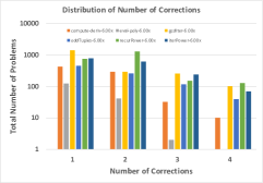
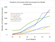
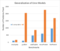
(a)	(b)	(c)

Figure 13: (a) The number of incorrect problem that require different number of corrections, (b) the number of problems corrected with adding rules to the error models, and (c) the performance of compute-deriv error model on other problems.

Benchmark	Total	Syntax	Test Set	Correct	Incorrect	Generated	Average	Median
	Attempts	Errors			Attempts	Feedback	Time(in s)	Time(in s)
prodBySum-6.00	1056	16	1040	772	268	218 (81.3%)	2.49s	2.53s
oddTuples-6.00	2386	1040	1346	1002	344	185 (53.8%)	2.65s	2.54s
computeDeriv-6.00	144	20	124	21	103	88 (85.4%)	12.95s	4.9s
evalPoly-6.00	144	23	121	108	13	6 (46.1%)	3.35s	3.01s
computeDeriv-6.00x	4146	1134	3012	2094	918	753 (82.1%)	12.42s	6.32s
evalPoly-6.00x	4698	1004	3694	3153	541	167 (30.9%)	4.78s	4.19s
oddTuples-6.00x	10985	5047	5938	4182	1756	860 (48.9%)	4.14s	3.77s
iterPower-6.00x	8982	3792	5190	2315	2875	1693 (58.9%)	3.58s	3.46s
recurPower-6.00x	8879	3395	5484	2546	2938	2271 (77.3%)	10.59s	5.88s
iterGCD-6.00x	6934	3732	3202	214	2988	2052 (68.7%)	17.13s	9.52s
stock-market-I(C#)	52	11	41	19	22	16 (72.3%)	7.54s	5.23s
stock-market-II(C#)	51	8	43	19	24	14 (58.3%)	11.16s	10.28s
restaurant rush (C#)	124	38	86	20	66	41 (62.1%)	8.78s	8.19s

Table 1: The percentage of student attempts corrected and the time taken for correction for the benchmark problems.

Number of Corrections

The number of student attempts that require different number of corrections are shown in Figure 13(a). We observe from the figure that a large fraction of the problems require 3 and 4 coordinated corrections, and to provide feedback on such attempts, we need a technology like ours that can symbolically encode the outcome of different corrections on all input values.

Repetitive Mistakes

In this experiment, we validate our hypothesis that students make similar mistakes while solving a given problem. The graph in Figure 13(b) shows the number of student attempts corrected as more rules are added to the error model of the benchmark problems. As can be seen in the figure, adding a single rule to the error model can lead to correction of hundreds of attempts.

Generalization of Error Models

In this experiment, we check the hypothesis that whether the correction rules generalize across problems of similar kind. The result of running the compute-deriv error model on other benchmark problems is shown in figrefgraphs(c). As expected, it does not perform as well as the problem-specific error models, but it does suffice to fix a fraction of the incorrect attempts and also provides a good starting point to add more problem-specific rules.

6 Related Work

In this section, we describe several related work to our technique from the areas of automated programming tutors, automated program repair, fault localization, automated debugging and program synthesis.

6.1 AI based programming tutors

There has been a lot of work done in the AI community for building automated tutors for helping novice programmers learn programming by providing feedback about semantic errors. These tutoring systems can be categorized into the following two major classes:

Code-based matching approaches: LAURA Adam and Laurent [1980] converts teacher’s and student’s program into a graph based representation and compares them heuristically by applying program transformations while reporting mismatches as potential bugs. TALUS Murray [1987] matches a student’s attempt with a collection of teacher’s algorithms. It first tries to recognize the algorithm used and then tentatively replaces the top-level expressions in the student’s attempt with the recognized algorithm for generating correction feedback. The problem with these approach is that the enumeration of all possible algorithms (with its variants) for covering all corrections is very large and tedious on part of the teacher.

Intention-based matching approaches: LISP tutor Farrell et al. [1984] creates a model of the student goals and updates it dynamically as the student makes edits. The drawback of this approach is that it forces students to write code in a certain pre-defined structure and limits their freedom. MENO-II Soloway et al. [1981] parses student programs into a deep syntax tree whose nodes are annotated with plan tags. This annotated tree is then matched with the plans obtained from teacher’s solution. PROUST Johnson and Soloway [1985], on the other hand, uses a knowledge base of goals and their corresponding plans for implementing them for each programming problem. It first tries to find correspondence of these plans in the student’s code and then performs matching to find discrepancies. CHIRON Sack et al. [1992] is its improved version in which the goals and plans in the knowledge base are organized in a hierarchical manner based on their generality and uses machine learning techniques for plan identification in the student code. These approaches require teacher to provide all possible plans a student can use to solve the goals of a given problem and do not perform well if the student’s attempt uses a plan not present in the knowledge base.

Our approach performs semantic equivalence of student’s attempt and teacher’s solution based on exhaustive bounded symbolic verification techniques and makes no assumptions on the algorithms or plans that students can use for solving the problem. Moreover, our approach is modular with respect to error models; the local correction rules are provided in a declarative manner and their complex interactions are handled by the solver itself.

6.2 Automated Program Repair

K$\ddot{o}$nighofer et. al. Könighofer and Bloem [2011] present an approach for automated error localization and correction of imperative programs. They use model-based diagnosis to localize components that need to be replaced and then use a template-based approach for providing corrections using SMT reasoning. Their fault model only considers the right hand side (RHS) of assignment statements as replaceable components. The approaches in Jobstmann et al. [2005]; Staber et al. [2005] frame the problem of program repair as a game between an environment that provides the inputs and a system that provides correct values for the buggy expressions such that the specification is satisfied. These approaches only support simple corrections (e.g. correcting RHS side of expressions) in the fault model as they aim to repair large programs with arbitrary errors. In our setting, we exploit the fact that we have access to the dataset of previous student mistakes that we can use to construct a concise and precise error model. This enables us to model more sophisticated transformations such as introducing new program statements, replacing LHS of assignments etc. in our error model. Our approach also supports minimal cost changes to student’s programs where each error in the model is associated with a certain cost, unlike the earlier mentioned approaches.

Mutation-based program repair Debroy and Wong [2010] performs mutations repeatedly to statements in a buggy program in order of their suspiciousness until the program becomes correct. The large state space of mutants ($10^{12}$) makes this approach infeasible. Our approach uses a symbolic search for exploring correct solutions over this large set. There are also some genetic programming approaches that exploit redundancy present in other parts of the code for fixing faults Arcuri [2008]; Forrest et al. [2009]. These techniques are not applicable in our setting as such redundancy is not present in introductory programming problems.

6.3 Automated Debugging and Fault localization

Techniques like Delta Debugging  Zeller and Hildebrandt [2002] and QuickXplain Junker [2004] aim to simplify a failing test case to a minimal test case that still exhibits the same failure. Our approach can be complemented with these techniques to restrict the application of rewrite rules to certain failing parts of the program only. There are many algorithms for fault localization Ball et al. [2003]; Groce et al. [2006] that use the difference between faulty and successful executions of the system to identify potential faulty locations. Jose et. al. Jose and Majumdar [2011] recently suggested an approach that uses a MAX-SAT solver to satisfy maximum number of clauses in a formula obtained from a failing test case to compute potential error locations. These approaches, however, only localize faults for a single failing test case and the suggested error location might not be the desired error location, since we are looking for common error locations that cause failure of multiple test cases. Moreover, these techniques provide only a limited set of suggestions (if any) for repairing these faults.

6.4 Program Synthesis

Program synthesis has been used recently for many applications such as synthesis of efficient low-level code Solar-Lezama et al. [2005]; Kuncak et al. [2010], inference of efficient synchronization in concurrent programs Vechev et al. [2010], snippets of excel macros Gulwani et al. [2012], relational data structures Hawkins et al. [2011, 2012] and angelic programming Bodík et al. [2010]. The Sketch tool Solar-Lezama et al. [2005]; Solar-Lezama [2008] takes a partial program and a reference implementation as input and uses constraint-based reasoning to synthesize a complete program that is equivalent to the reference implementation. In general cases, the template of the desired program as well as the reference specification is unknown and puts an additional burden on the users to provide them; in our case we use the student’s solution as the template program and teacher’s solution as the reference implementation. A recent work by Gulwani et. al. Gulwani et al. [2011] also uses program synthesis techniques for automatically synthesizing solutions to ruler/compass based geometry construction problems. Their focus is primarily on finding a solution to a given geometry problem whereas we aim to provide feedback on a given programming exercise solution.

7 Conclusions

In this paper, we presented a new technique of automatically providing feedback for introductory programming assignments that can complement manual and test-cases based techniques. The technique uses an error model describing the potential corrections and constraint-based synthesis to compute minimal corrections to student’s incorrect solutions. We have evaluated our technique on a large set of benchmarks and it can correct $65\%$ of incorrect solutions. We believe this technique can provide a basis for providing automated feedback to hundreds of thousands of students learning from online introductory programming courses that are being taught by MITx and Udacity.

References

- [1] Automated feedback generation for introductory programming assignments. Technical report. supplementary material.
- Adam and Laurent [1980] A. Adam and J.-P. H. Laurent. LAURA, A System to Debug Student Programs. Artif. Intell., 15(1-2):75–122, 1980.
- Arcuri [2008] A. Arcuri. On the automation of fixing software bugs. In ICSE Companion, 2008.
- Ball et al. [2003] T. Ball, M. Naik, and S. K. Rajamani. From symptom to cause: localizing errors in counterexample traces. In POPL, 2003.
- Bodík et al. [2010] R. Bodík, S. Chandra, J. Galenson, D. Kimelman, N. Tung, S. Barman, and C. Rodarmor. Programming with angelic nondeterminism. In POPL, 2010.
- Debroy and Wong [2010] V. Debroy and W. Wong. Using mutation to automatically suggest fixes for faulty programs. In ICST, 2010.
- Ertmer et al. [2007] P. Ertmer, J. Richardson, B. Belland, D. Camin, P. Connolly, G. Coulthard, K. Lei, and C. Mong. Using peer feedback to enhance the quality of student online postings: An exploratory study. Journal of Computer-Mediated Communication, 12(2):412–433, 2007.
- Farrell et al. [1984] R. G. Farrell, J. R. Anderson, and B. J. Reiser. An interactive computer-based tutor for lisp. In AAAI, 1984.
- Forrest et al. [2009] S. Forrest, T. Nguyen, W. Weimer, and C. L. Goues. A genetic programming approach to automated software repair. In GECCO, 2009.
- Groce et al. [2006] A. Groce, S. Chaki, D. Kroening, and O. Strichman. Error explanation with distance metrics. STTT, 8(3):229–247, 2006.
- Gulwani et al. [2008] S. Gulwani, S. Srivastava, and R. Venkatesan. Program analysis as constraint solving. In PLDI, 2008.
- Gulwani et al. [2011] S. Gulwani, V. A. Korthikanti, and A. Tiwari. Synthesizing geometry constructions. In PLDI, 2011.
- Gulwani et al. [2012] S. Gulwani, W. R. Harris, and R. Singh. Spreadsheet data manipulation using examples. In CACM, 2012.
- Hawkins et al. [2011] P. Hawkins, A. Aiken, K. Fisher, M. C. Rinard, and M. Sagiv. Data representation synthesis. In PLDI, 2011.
- Hawkins et al. [2012] P. Hawkins, A. Aiken, K. Fisher, M. C. Rinard, and M. Sagiv. Concurrent data representation synthesis. In PLDI, 2012.
- Jobstmann et al. [2005] B. Jobstmann, A. Griesmayer, and R. Bloem. Program repair as a game. In CAV, pages 226–238, 2005.
- Johnson and Soloway [1985] W. L. Johnson and E. Soloway. Proust: Knowledge-based program understanding. IEEE Trans. Software Eng., 11(3):267–275, 1985.
- Jose and Majumdar [2011] M. Jose and R. Majumdar. Cause clue clauses: error localization using maximum satisfiability. In PLDI, 2011.
- Junker [2004] U. Junker. QUICKXPLAIN: preferred explanations and relaxations for over-constrained problems. In AAAI, 2004.
- Könighofer and Bloem [2011] R. Könighofer and R. P. Bloem. Automated error localization and correction for imperative programs. In FMCAD, 2011.
- Kuncak et al. [2010] V. Kuncak, M. Mayer, R. Piskac, and P. Suter. Complete functional synthesis. PLDI, 2010.
- Murray [1987] W. R. Murray. Automatic program debugging for intelligent tutoring systems. Computational Intelligence, 3:1–16, 1987.
- Sack et al. [1992] W. Sack, E. Soloway, and P. Weingrad. From PROUST to CHIRON: Its design as iterative engineering: Intermediate results are important! In In J.H. Larkin and R.W. Chabay (Eds.), Computer-Assisted Instruction and Intelligent Tutoring Systems: Shared Goals and Complementary Approaches., pages 239–274, 1992.
- Solar-Lezama [2008] A. Solar-Lezama. Program Synthesis By Sketching. PhD thesis, EECS Dept., UC Berkeley, 2008.
- Solar-Lezama et al. [2005] A. Solar-Lezama, R. Rabbah, R. Bodik, and K. Ebcioglu. Programming by sketching for bit-streaming programs. In PLDI, 2005.
- Soloway et al. [1981] E. Soloway, B. P. Woolf, E. Rubin, and P. Barth. Meno-II: An Intelligent Tutoring System for Novice Programmers. In IJCAI, 1981.
- Srivastava et al. [2010] S. Srivastava, S. Gulwani, and J. Foster. From program verification to program synthesis. POPL, 2010.
- Staber et al. [2005] S. S. Staber, B. Jobstmann, and R. P. Bloem. Finding and fixing faults. In Correct Hardware Design and Verification Methods, Lecture notes in computer science, pages 35 – 49, 2005.
- Vechev et al. [2010] M. Vechev, E. Yahav, and G. Yorsh. Abstraction-guided synthesis of synchronization. In POPL, New York, NY, USA, 2010. ACM.
- Zeller and Hildebrandt [2002] A. Zeller and R. Hildebrandt. Simplifying and isolating failure-inducing input. IEEE Transactions on Software Engineering, 28:183–200, 2002.