Dissecting the FEAST algorithm for generalized eigenproblems

Abstract

We analyze the FEAST method for computing selected eigenvalues and eigenvectors of large sparse matrix pencils. After establishing the close connection between FEAST and the well-known Rayleigh–Ritz method, we identify several critical issues that influence convergence and accuracy of the solver: the choice of the starting vector space, the stopping criterion, how the inner linear systems impact the quality of the solution, and the use of FEAST for computing eigenpairs from multiple intervals. We complement the study with numerical examples, and hint at possible improvements to overcome the existing problems.

1 Introduction

In 2009, Polizzi introduced the FEAST solver for generalized Hermitian definite eigenproblems [1]. FEAST was conceived as an algorithm for electronic structure calculations, and then evolved into a general purpose solver. In this paper we describe the mathematical structure of the algorithm and conduct an investigation of its robustness and accuracy.

FEAST belongs to a family of iterative solvers based on the contour integration of a density-matrix representation of quantum mechanics; the result of the integration is a subspace projector that plays a central role in a Rayleigh–Ritz method. The prominent member in this family was developed by Sakurai and Sugiura in 2003 [2]; this work, which inspired a number of generalizations and high-performance implementations [3, 4], targets non-Hermitian eigenproblems. By contrast, FEAST promises to deliver performance on sparse Hermitian problems. Such problems can be solved by a number of alternative packages like ARPACK [5] and TRLan [6] and the solver implemented in PARSEC [7, 8].

Since in ab-initio electronic calculations typically one is interested in the lowest part of the eigenspectrum, we investigate FEAST’s behavior for the computation of a subset of eigenpairs lying inside a given interval. Additionally, we study its strengths and weaknesses when a large portion or all of the spectrum is sought after. In our analysis, we use a number of matrices from practical applications. From our experiments, we found that while for specific scenarios FEAST is accurate and reliable, in general it lacks robustness.

Our analysis touches upon three main features of the solver: 1) critical input parameters, 2) the stopping criterion, and 3) the quality of the results.

• In addition to a search interval, FEAST’s interface requires the user to specify the number of eigenvalues present within the interval. Although in some ab-initio simulations this number can be accurately estimated, in general it is not possible to obtain it cheaply; since the completeness of the computed eigenpairs greatly depends on it, this initial guess is critical. The user can also specify a starting vector base which FEAST uses to initialize the solver: while by default FEAST uses a random set of vectors, the convergence rate of the solver greatly depends on the actual choice. We elaborate on how different starting bases affect convergence speed and robustness.

• The original implementation of FEAST employs a stopping criterion based on monitoring relative changes in the sum of all computed Ritz values. We identify cases where this criterion does not reflect the actual convergence and propose an alternative criterion based on per-eigenpair residuals.

• We analyze the quality of the solution computed by FEAST by means of residuals and orthogonality. On the one hand we found that the achievable residuals are affected by the accuracy of the linear solver used within the algorithm. On the other hand, we distinguish between local and global orthogonality, i. e., orthogonality among eigenvectors that were computed with a single interval, and among vectors from separate intervals, respectively. While the local orthogonality is guaranteed by the Rayleigh–Ritz method, depending on the spectrum of the eigenproblem the global orthogonality might suffer.

The paper is organized as follows. In Section 2 we illustrate the underlying mathematical structure of the algorithm. Section 3 contains experiments and analysis concerning the different aspects of the solver. Section 4 examines the suitability of FEAST as a building-block for a general purpose solver, working on multiple intervals to compute a larger portion of the spectrum. We conclude in Section 5 suggesting improvements to broaden FEAST’s applicability.

2 FEAST and the Rayleigh–Ritz method

Let us consider the generalized eigenproblem $Ax=\lambda Bx$, with Hermitian matrix $A\in\mathbb{C}^{n\times n}$ and Hermitian positive definite $B\in\mathbb{C}^{n\times n}$. The objective is to compute the eigenpairs whose eigenvalues lie in a given interval $I_{\lambda}=[\underline{\lambda},\overline{\lambda}]$. Since FEAST is an instantiation of the Rayleigh–Ritz method, we start with a short review.

In the following, in order to denote an eigenpair $(\lambda,x)$ with $\lambda\in I_{\lambda}$, we will sloppily say that the eigenpair is in the interval $I_{\lambda}$.

2.1 Rayleigh–Ritz theorem

We present the Rayleigh–Ritz method in its orthonormal version, which ensures a minimal residual. The method relies on the following theorem.

Theorem 2.1 (Rayleigh–Ritz, [9])

Let $\mathcal{U}$ be a subspace containing an eigenspace $\mathcal{X}\subset\mathcal{U}$ of the generalized eigenproblem $Ax=\lambda Bx$. Let $U$ be a basis of vectors for $\mathcal{U}=\mathop{\mathrm{missing}}{span}\nolimits(U)$, $U^{I}$ a left inverse of $U$, and $A_{U}=U^{I}AU$, $B_{U}=U^{I}BU$ the so-called Rayleigh quotients for $A$ and $B$. If $(\Lambda,W)$ (${\Lambda}=\mathop{\mathrm{missing}}{diag}\nolimits(\lambda_{1},\lambda_{2},\ldots)$) are primitive Ritz pairs of the reduced problem, i. e., $A_{U}W=B_{U}W\Lambda$, then $(\Lambda,X)$ are Ritz pairs for the original eigenproblem with $X=UW$ and $\mathop{\mathrm{missing}}{span}\nolimits(X)=\mathcal{X}$.

In a neighborhood of the exact solutions for the primitive Ritz pair, we expect that the Rayleigh–Ritz theorem also applies approximately, leading to the following strategy.

1. Find a suitable basis $U$ for $\mathcal{U}$.

2. Compute the Rayleigh quotients $A_{U}=U^{I}\!AU$, $B_{U}=U^{I}\!BU$.

3. Compute the primitive Ritz pairs $(\widetilde{\Lambda},\widetilde{W})$ of $A_{U}W=B_{U}W\Lambda$.

4. Return the approximate Ritz pairs $(\widetilde{\Lambda},U\widetilde{W})$ of $AX=BX\Lambda$.

5. Check convergence criterion; if not satisfied, go back to Step 1.

Let us point out that obtaining an accurate approximation of $(\Lambda,X)$ is not an obvious consequence of computing primitive Ritz pairs. One must ensure that both Ritz values and the corresponding Ritz vectors converge to the desired eigenpairs. Conversely, it must hold that each eigenpair in $I_{\lambda}$ corresponds to a primitive Ritz pair in the same interval; see [9].

2.2 The algorithm

The FEAST algorithm implements the above Rayleigh–Ritz method, with a particular choice for computing $U$:

$$U:=\frac{1}{2\pi i}\int_{\mathcal{C}}\mathrm{d}z(zB-A)^{-1}BY,$$ (1)

where $\mathcal{C}$ is a curve in the complex plane enclosing the selected interval $I_{\lambda}$. The expression $(zB-A)^{-1}B$ is normally referred to as the eigenproblem’s resolvent; Formula (1) can be interpreted as the projection of the set of vectors $Y$ onto a subspace $\mathcal{U}$ containing the eigenspace. Pseudo-code for FEAST is provided in Algorithm 1.

Algorithm 1 Skeleton of the FEAST algorithm

1:An interval $I_{\lambda}=\left[\underline{\lambda},\overline{\lambda}\right]$ and an estimate $\widetilde{M}$ of the number of eigenvalues in $I_{\lambda}$.

2:$\hat{M}\leq\widetilde{M}$ eigenpairs in $I_{\lambda}$.

3:Choose $Y\in\mathbb{C}^{n\times\widetilde{M}}$ of rank $\widetilde{M}$ and compute $U:=\frac{1}{2\pi i}\int_{\mathcal{C}}\mathrm{d}z\ (zB-A)^{-1}B\,Y$;

4:Form the Rayleigh quotients $A_{U}:=U^{H}\!AU,\;B_{U}:=U^{H}\!BU$;

5:Solve the size-$\widetilde{M}$ generalized eigenproblem $A_{U}\widetilde{W}=B_{U}\widetilde{W}\widetilde{\Lambda}$;

6:Compute the approximate Ritz pairs $(\widetilde{\Lambda},\widetilde{X}:=U\cdot\widetilde{W})$;

7:If convergence is not reached then go to Step 3, with $Y:=\widetilde{X}$.

Having established the close connection between FEAST and the Rayleigh–Ritz method, the next section is devoted to the theoretical framework for the resolvent and the contour integration (1).

2.3 Integrating the resolvent

In this section we define the concept of resolvent and illustrate its functionality within the Rayleigh–Ritz method. The objective is to show that the subspace $U$ is approximated by the integral operator in Equation (1). We recall that a generalized Hermitian definite eigenproblem has $n$ real eigenvalues $\lambda_{1}$, …, $\lambda_{n}$ and $B$-orthonormal eigenvectors $x_{1}$, …, $x_{n}$.

Let us consider a single eigenpair $(\lambda_{k},x_{k})$, and let $z\in\mathbb{C}$. For $z\not=\lambda_{i},i\in\{1,\dots,n\}$,

$$B^{-1}(zB-A)x_{k}=(z-\lambda_{k})x_{k},$$

and

$$(zB-A)^{-1}Bx_{k}=(B^{-1}(zB-A))^{-1}x_{k}=(z-\lambda_{k})^{-1}x_{k}.$$ (2)

Define the resolvent operator $G(z)$ as

$$G(z):=(zB-A)^{-1}B$$

and let $\mathcal{C}_{k}$ be a closed curve in the complex plane enclosing only the eigenvalue $\lambda_{k}$. Thus, the integral

$$\frac{1}{2\pi i}\int_{\mathcal{C}_{k}}\mathrm{d}z\,G(z)x_{k}$$

equals the residue of $G(z)x_{k}$ localized at the pole in $\lambda_{k}$. Using Equation (2), we obtain

$$\frac{1}{2\pi i}\int_{\mathcal{C}_{k}}\mathrm{d}z\,(zB-A)^{-1}Bx_{k}=\frac{1}{2\pi i}\int_{\mathcal{C}_{k}}\frac{\mathrm{d}z}{z-\lambda_{k}}x_{k}=\frac{1}{2\pi i}2\pi ix_{k}=x_{k}.$$ (3)

By contrast, the residue around any other pole returns 0.

Now let $\mathcal{C}$ be a curve enclosing a subset $\{\lambda_{k}:k\in I\}$ of the eigenvalues. Combining Equations (3) for $k\in I$ and splitting the path integral over $\mathcal{C}$ into a sum of integrals over closed curves $\mathcal{C}_{k}$ containing just one eigenvalue $\lambda_{k}$ each, one obtains

$$\frac{1}{2\pi i}\int_{\mathcal{C}}\mathrm{d}z\,G(z)x_{j}=\sum_{k\in I}\frac{1}{2\pi i}\int_{\mathcal{C}_{k}}\mathrm{d}z\,G(z)x_{j}=\sum_{k\in I}\delta_{k,j}x_{j}=\left\{\begin{array}[]{ll}x_{j},&\mbox{if $j\in I$}\\ 0,&\mbox{otherwise}\end{array}\right..$$ (4)

So far we have shown how the projection operator acts on the full space of eigenvectors. This is a well known property of the resolvent of an eigenproblem [10, Ch. 3]. This property can also be visualized by combining the $B$-orthogonal eigenvectors $x_{k}$, $k\in I$, into an $n$-by-$|I|$ matrix $X$, and by comparing (4) with the application of the projector

$$Q=XX^{H}\ B=\sum_{k\in I}x_{k}x_{k}^{H}\ B\quad{\rm with}\quad Q^{2}=Q$$

to an eigenvector $x_{j}$,

$$Qx_{j}=\sum_{k\in I}(x_{k}x_{k}^{H})Bx_{j}=\sum_{k\in I}x_{k}\delta_{k,j}=\left\{\begin{array}[]{ll}x_{j},&\mbox{if $j\in I$}\\ 0,&\mbox{otherwise}\end{array}\right..$$

One then concludes that the operators $\frac{1}{2\pi i}\int_{\mathcal{C}}\mathrm{d}z\,G(z)$ and $Q$, when applied to a set of eigenvectors, produce the same results.

Let $Y=\{y_{1},y_{2},\dots,y_{M}\}$, then

$$\frac{1}{2\pi i}\int_{\mathcal{C}}\mathrm{d}z\ (zB-A)^{-1}\ BY=QY=XX^{H}BY$$

projects each $y_{j}$ onto the eigenspace $\mathcal{X}=\mathop{\mathrm{missing}}{span}\nolimits(X)$. In this sense, the matrix $U$ computed in Algorithm 1 is a reasonable attempt to fulfill the requirements of the Rayleigh–Ritz theorem. In practice, the integral (1) must be evaluated numerically, using a scheme such as Gauß–Legendre; for details we refer to the original publication [1] and to the literature on numerical integration, e. g.,  [11].

A numerical integration scheme leads to an approximation

$$\hat{U}\approx\frac{1}{2\pi i}\sum_{k=1}^{m}w_{k}(z_{k}B-A)^{-1}\ BY$$

where the points $z_{k}$ lie on the curve $\mathcal{C}$. The accuracy of the approximation, as well as the computational complexity, are determined by the number of integration points. In practice, Gaussian rules with 7–10 nodes already achieve satisfactory results. For each integration point, a linear system $(z_{k}B-A)\hat{U}_{k}=BY$ of size $N$ with $\widetilde{M}$ right-hand sides must be solved.

If the curve $\mathcal{C}$ is chosen to be symmetric with respect to the real axis (e.g., a circle or ellipse), then considerable computational savings are possible. In this case the numerical integration must cover only the half-curve in the upper complex half-plane due to the symmetry $G(\bar{z})=G^{H}(z)$ [1].

3 Analysis and experiments for the FEAST algorithm

In this section we discuss the issues arising when employing FEAST to compute the eigenpairs in a single interval: size and choice of the search space, stopping criteria and impact of the linear solver on the accuracy of the solution.

3.1 Size of the search space $\mathcal{U}$

Section 2.3 shows that the size of the eigenspace $\mathcal{X}$ is determined by the number $M$ of columns of $U$ which in turn corresponds to the number of columns of $Y$. This number is equivalent to the number $M$ of eigenvalues (counting multiplicities) lying in the given interval $I_{\lambda}$. In practice, $M$ is not known a priori, and an estimate $\widetilde{M}$ has to be used instead. In the following, we discuss the consequences of the cases $\widetilde{M}>M$ and $\widetilde{M}<M$.

Case $\widetilde{M}>M$. If the estimate is larger than the actual number of eigenvalues in $I_{\lambda}$, then the spectral projector $Q$ has rank $M$, and thus the $n$-by-$\widetilde{M}$ matrix $U=QY$ is rank-deficient and does not have a full rank left inverse. As a direct consequence, $B_{U}$ is rank deficient, and the eigenpairs of the reduced eigenproblem might be incomplete and not necessarily $B$-orthogonal.

In the original implementation of FEAST, the rank deficiency is detected by measuring the “positive definiteness” of $B_{U}$ through a Cholesky decomposition. A drawback of this approach is that it does not indicate which of the columns of $U$ are linearly independent, forcing one to select a subset arbitrarily. This, in turn, might result in the presence of spurious eigenpairs. A reliable, but more expensive, approach consists of computing an SVD or a (rank-revealing) QR decomposition of the matrix $U$ [12]. Since the rank of $U$ equals the number of eigenvalues in $I_{\lambda}$, such a rank-revealing decomposition can be used to safely restart the process with $Y=\bar{U}X$, where $\bar{U}$ includes the linearly independent columns of $U$.

Case $\widetilde{M}<M$. The space spanned by $U$ does not contain the whole eigenspace corresponding to the eigenvalues within the integration contour, and therefore the vectors generated by integrating the resolvent fail to span $\mathcal{X}$.

The following experiment illustrates the behavior of FEAST for different numbers $\widetilde{M}$.

Experiment 3.1

We consider a size-$1059$ matrix $A=\texttt{LAP\_CIT\_1059}$ from modelling cross-citations in scientific publications, and $B=I$. In this test we search for $\widetilde{M}=1,\ldots,450$ eigenpairs with eigenvalues in an interval $I_{\lambda}$ containing the $M=300$ lowest eigenvalues. The maximum number of iterations allowed for FEAST is 20.

The left panel of Figure 1 shows the number of iterations necessary for FEAST to calculate all eigenpairs within $I_{\lambda}$ with sufficiently small residual $\left\|Ax-\lambda Bx\right\|\leq\varepsilon\cdot n\cdot\max\{\left\lvert\underline{\lambda}\right\rvert,\left\lvert\overline{\lambda}\right\rvert\}$, as a function of $\widetilde{M}$. An iteration count of 20 typically implies that either none or not all eigenpairs converged within these 20 iterations. The right panel shows the residual span for all computed eigenpairs with eigenvalues in the interval after the respective number of iterations (20 or fewer, if convergence was reached beforehand). Again these numbers are given as a function of $\widetilde{M}$. We see that, leaving aside the very small region around the exact eigenspace size, either all or none of the eigenpairs show a sufficiently small residual. While for $\widetilde{M}<M$ no eigenpairs converge and especially the minimum residuals are large, for $\widetilde{M}>M$ also the maximum residuals begin to drop significantly and typically all eigenpairs may converge if only enough iterations are performed. With $\widetilde{M}$ just slightly larger than $M$, all eigenpairs reach convergence within few iterations.

For a better understanding of the evolution of the computed eigenspace, we monitored the largest canonical angle $\sphericalangle\left(X^{(i)},X_{I_{\lambda}}\right)$ [12, p. 603] between the current approximate eigenspace $X^{(i)}$ and the exact eigenspace $X_{I_{\lambda}}$, as well as the angle $\sphericalangle\left(X^{(i)},X^{(i-1)}\right)$ between the current and the previous iterate. Figure 2 provides these angles for three values of $\widetilde{M}$, $\widetilde{M}=250,\;\widetilde{M}=300$ and $\widetilde{M}=350$. In this last case, after five iterations the computed eigenspace contains the exact one and does not vary anymore; these two facts imply convergence. By contrast, the curves for $\widetilde{M}=250$ indicate that while the computed eigenspace becomes contained in the exact one after more than 20 iterations, it keeps varying, never to reach convergence. Interestingly, the worst convergence with respect to the exact eigenspace seems to occur for $\widetilde{M}=300$. This can be intuitively understood by the fact that two subspaces of the same dimension need to be identical in order to have an angle of zero between each other.

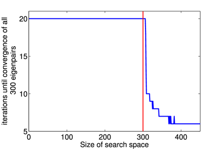
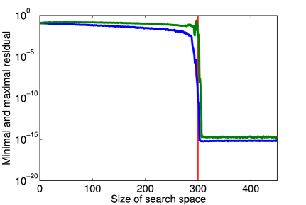
Figure 1: Left: Number of necessary iterations. Right: Minimal (lower line) and maximal (upper line) residual.

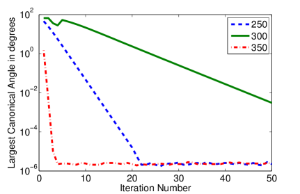
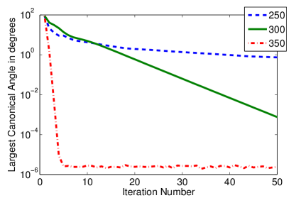
Figure 2: Canonical angles (left: between current iterate $X^{(i)}$ and exact eigenspace $X_{I}$; right: between current iterate $X^{(i)}$ and previous iterate $X^{(i-1)}$) in degrees for $\widetilde{M}=250,300,350$.

3.2 Choice of the starting basis $Y$

The choice of the starting basis $Y\in\mathbb{C}^{n\times\widetilde{M}}$ in line 3 of Algorithm 1 plays a critical role in the unfolding of the algorithm: most importantly, $Y$ has to include components along $U$, so that its projection through $Q$ spans $\mathcal{X}$. Vice versa, if one or more of the columns of $Y$ are $B$-orthogonal to the space $\mathcal{U}$, then the corresponding columns of $U=QY$ will be zero. If a good initial guess for the eigenvectors of $(A,B)$ is available, then it can used as the starting base $Y$; otherwise the typical choice is a base of random vectors.

Experiment 3.2

We used FEAST with $\widetilde{M}=450$ to compute the $M=300$ lowest eigenvalues and corresponding eigenvectors of the matrix pencil $(A=\texttt{LAP\_CIT\_1059},B=I)$. These eigenvalues are simple and sufficiently far away from the only multiple eigenvalue, which is zero. With a fixed random starting basis $Y$, four iterations were sufficient to compute all wanted eigenpairs with residuals $\left\|Ax_{j}-\lambda_{j}Bx_{j}\right\|\leq 5.5\times 10^{-15}$. Then we projected out the ten eigenvectors corresponding to the $10$ lowest eigenvalues via $Y:=(I-X_{1:10}X_{1:10}^{T})\cdot Y$. It took seven iterations for the lowest $290$ eigenpairs to converge, and nine more iterations for other nine. One eigenpair did not converge within the limit of 20 iterations. Convergence took place “from top to bottom”, i. e., the eigenpairs $11,\ldots,300$ converged first, then the eigenpairs $2,\ldots,10$. The smallest eigenvalue did not converge within the iteration limit.

In general, thanks to round-off errors, convergence could still be reached in most of our tests. In fact even though some components were zeroed out, the floating point arithmetic causes almost zero entries to grow as the computation progresses. Convergence is then reached with noticeably more iterations.

3.3 Stopping criteria

Algorithm 1 relies on a stopping criterion to determine whether the eigenpairs are computed to a sufficient degree of accuracy. Such a criterion must balance cost and effectiveness. In the original implementation [1], FEAST monitors convergence through the change in the sum of the computed eigenvalues; more precisely, a relative criterion of the form

$$\frac{\left\lvert\mathsf{trace}_{k}-\mathsf{trace}_{k-1}\right\rvert}{\left\lvert\mathsf{trace}_{k}\right\rvert}<\mathrm{TOL}$$ (5)

is used, where $\mathsf{trace}_{k}$ denotes the sum of the Ritz values in the $k$th iteration lying in the search interval and $\mathrm{TOL}$ is a user tolerance. Criterion (5) raises three problems.

First, its denominator might be zero or close to, causing severe numerical instabilities. Such a scenario arises, for instance, when all the eigenvalues in the search interval are zero. Second, the number $\mathsf{trace}_{k}$ can be (almost) constant for two consecutive values of $k$, stopping FEAST even if the residuals are still large. The third problem is of a more general nature: if the algorithm stagnates before the considered eigenpairs converge, all criteria that are based only on the change in the eigenvalues might still signal convergence. It is not hard to construct examples where this happens [9].

As an alternative criterion we propose a per-eigenpair residual that depends on the search interval: a Ritz pair has converged if it fulfills the inequality

$$\left\|Ax-Bx\lambda\right\|\leq\varepsilon\cdot n\cdot\max\{\left\lvert\underline{\lambda}\right\rvert,\left\lvert\overline{\lambda}\right\rvert\}.$$ (6)

The extra cost of this criterion is one matrix–vector product per vector because $Bx$ is needed anyway to compute $Y$ in the next iteration, or, if sparsity is not exploited, $\mathcal{O}(\widetilde{M}^{2}n)$ operations since $Ax=(AU)w$, with $AU$ reused from Step 2 of the FEAST algorithm. If $\max\{\left\lvert\underline{\lambda}\right\rvert,\left\lvert\overline{\lambda}\right\rvert\}$ is too small, e. g., when only eigenpairs with zero eigenvalues are sought after, one may replace this quantity by an estimate for $\left\|B^{-1}A\right\|$, which is the magnitude of the largest eigenvalue of the problem and might be obtained by some auxiliary routine (e. g., by some steps of a Lanczos method, see [13]).

Let us consider a matrix with spectrum symmetric with respect to zero, and choose the search interval to be symmetric around zero. If summed, the computed Ritz values cancel themselves pairwise, thus $\mathsf{trace}_{k}$ is approximately zero. When FEAST is applied to such a matrix, the trace criterion signals convergence when the difference in (5) comes close enough to zero; in this case, the ratio (5) holds no information about convergence. From multiple tests with random starting bases, we experienced that it took between 7 and 100 iterations for criterion (5) to signal convergence. By contrast, criterion (6) dropped below $10^{-15}$ always after 6 iterations.

In an additional test, we ran FEAST on a symmetric matrix of size $470$, seeking the known $57$-fold eigenvalue $1$. Here we chose the search interval symmetrically around $1$, and $\widetilde{M}=120>M$. After five iterations, (5) was $1.2\times 10^{-16}$, effectively halting the computation, although the residuals (6) were still of order $10^{-9}$ to $10^{-12}$. The right hand side of (6) was about $10^{-13}$ in this example, meaning that none of the residuals was satisfactory small.

3.4 The impact of the linear solver on residuals and orthogonality

As seen in Section 2.3, the computation of the basis according to (1) involves solving several linear systems of the form

$$(zB-A)V=BY$$ (7)

for $V$. The particular values of the integration points $z$ depend on the method chosen for numerical integration, which is not discussed here. Typically, $z$ will be a complex number near the spectrum of $(A,B)$. Recall that (7) is a linear system with $\widetilde{M}$ right hand sides. In principle, any linear solver can be used. Direct solvers, e. g., Gaussian elimination based, can be prohibitively expensive because for each value of $z$ we need to factorize $zB-A$, which may be an $\mathcal{O}(n^{3})$ process.

The methods of choice for solving large sparse linear systems without further knowledge about the underlying problem are Krylov subspace methods; for a review see, e. g., [10]. Here we cannot give a detailed discussion, but let us remark that the convergence of Krylov subspace methods depends on several parameters. First, the best convergence results can be expected for Hermitian matrices since this property can be exploited. Unfortunately, (7) typically has a non-real diagonal and therefore is not a Hermitian problem. (However, if $B=I$ then the matrix $zI-A$ is shifted Hermitian, so methods for shifted systems may be applicable [14].) Second, the convergence for a fixed method typically depends on the structure of the spectrum of the matrix. The eigenvalues of $zB-A$ are scattered over the complex plane so that no good convergence results can be inferred. Third, the condition number $\left\|(zB-A)^{-1}\right\|\cdot\left\|zB-A\right\|$ of the system plays an important role and is often large for (7), since $z$ can be very close to the spectrum of $(A,B)$. For these reasons, standard Krylov subspace solvers may need a large number of iterations to converge. This expectation was confirmed by our experiments. The need for an effective preconditioner is apparent, and its development is part of further research.

Another way to speed up the linear solvers is to terminate them before full convergence is reached. Thus the question arises how accurately the systems (7) need to be solved in order to obtain eigenpairs of sufficient quality in a reasonable number of FEAST iterations. We therefore investigated the effect of the accuracy in the solution of linear systems on the ultimately achievable per-eigenpair residuals and the orthogonality of the eigenvectors, as well as on the number of FEAST iterations.

Experiment 3.3

We applied Algorithm 1 to the matrix pair ($A$,$B$), where $A=\texttt{LAP\_CIT\_395}$ arises in the modelling of cross-citations in scientific publications, and $B$ was chosen to be a diagonal matrix with random entries. We calculated the eigenpairs corresponding to the $10$ largest eigenvalues. The linear systems were solved column-by-column by running GMRES [10] until $\left\|(zB-A)v_{j}-By_{j}\right\|/\left\|r^{0}_{j}\right\|\leq\varepsilon_{\mathrm{lin}}$, where $r^{0}_{j}$ is the starting residual. Figure 3 reveals that the residual bounds that were required in the solution of the inner linear systems translated almost one-to-one into the residuals of the Ritz pairs. Even for a rather large bound such as $\varepsilon_{\mathrm{lin}}=10^{-6}$, the FEAST algorithm still converged (even though to a quite large residual). For the orthogonality of the computed eigenvectors $x_{j}$, the situation was different. After $20$ FEAST iterations, an orthogonality level $\max_{i\neq j}\left\lvert x_{i}^{H}Bx_{j}\right\rvert$ of order $10^{-15}$ could be reached for each of the bounds $\varepsilon_{\mathrm{lin}}=10^{-6},10^{-8},10^{-10},10^{-12}$ in the solution of the linear systems. Thus the achievable orthogonality does not seem to be very sensitive to the accuracy of the linear solves. It also did not deteriorate significantly for a larger number of desired eigenpairs.

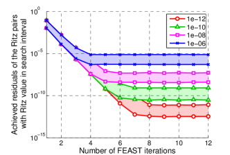
Figure 3: Range of all residuals among all Ritz pairs in $I_{\lambda}$ for four different residual bounds $\varepsilon_{\mathrm{lin}}$ in the linear solver.

4 FEAST for multiple intervals

Using FEAST for computing a large number $M$ of eigenpairs is not recommended since the complexity grows at least as $\mathcal{O}(nM^{2})$ due to the matrix–matrix products in Steps 2 and 4 of Algorithm 1, or $\mathcal{O}(n^{2}M)$ if sparsity is not exploited, because $\mathcal{O}(M)$ matrix–vector products must be computed. (In fact, if $M$ approaches $n$ then just Step 3 of Algorithm 1 has roughly the same complexity as the computation of the full eigensystem of the original problem.) However, as already hinted at in [1], FEAST’s ability to determine the eigenpairs in a specified interval makes it an attractive building block to compute the eigenpairs by subdividing the search interval $I_{\lambda}$ into $K$ subintervals $I_{\lambda}^{(1)},\ldots,I_{\lambda}^{(K)}$ and applying the algorithm—possibly in parallel—to each one of them.

In the following we report on issues concerning the orthogonality of eigenvectors coming from different subintervals. It is well known that eigenvectors computed independently from each other tend to have worse orthogonality than those obtained in a block-wise manner. Furthermore, the quality of the results depends on the internal structure of the spectrum, namely the relative distances between the eigenvalues. For more details, see, e. g., [13].

In the following we distinguish between global and local orthogonality, according to the definitions

$$\mathsf{orth}_{\mathrm{global}}=\max_{i\neq j,\;\lambda_{i},\lambda_{j}\in I_{\lambda}}\left\lvert x_{i}^{H}Bx_{j}\right\rvert\quad{\rm and}\quad\mathsf{orth}_{k}=\max_{i\neq j,\;\lambda_{i},\lambda_{j}\in I_{\lambda}^{(k)}}\left\lvert x_{i}^{H}Bx_{j}\right\rvert.$$

Note that $\mathsf{orth}_{\mathrm{global}}$ denotes the worst orthogonality among all computed eigenvectors, while $\mathsf{orth}_{k}$ describes the orthogonality achieved locally for the $k$th subinterval $I_{\lambda}^{(k)}$. The next two experiments reveal quite different behavior, depending on the presence of clusters and on the choice of subintervals.

Experiment 4.1

In this experiment we calculate the $800$ lowest eigenpairs of the size-$1473$ matrix pair (bcsstk11, bcsstm11) from the Matrix Market (http://math.nist.gov/MatrixMarket/). The corresponding eigenvalues range from $10.5$ to $3.8\times 10^{7}$ and are not clustered. We utilize different numbers of subintervals, $K=1,\ldots,5$, and $K=10$. Figure 4 shows that while the local orthogonality is high and maintained as the number of intervals increases, the global one degrades by two or more orders of magnitude.

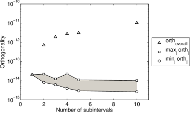
Figure 4: Global orthogonality and range of local orthogonality $\mathsf{orth}_{j}$ for $K=1,\ldots,5$ and $K=10$.

Experiment 4.2

In this test we consider a real unreduced tridiagonal matrix $A$ of size $2003$. Its eigenvalues are simple, even though some are tightly clustered; see the top plots in Figure 5. The objective is to compute the 300 largest eigenpairs. To this end we initially split the interval $I_{\lambda}=\left[\lambda_{1704},\;\lambda_{2003}\right]$ into $I_{\lambda}^{(1)}=[\lambda_{1704},\mu]$ and $I_{\lambda}^{(2)}=[\mu,\lambda_{2003}]$, with $\mu=\lambda_{1825}\approx 0.448\times 10^{-3}$ chosen within a a cluster of $99$ eigenvalues. The relative gap between eigenvalue $\lambda_{1825}$ and its neighbors is of about $10^{-12}$ (i. e., agreement to roughly eleven leading decimal digits). A sketch of the eigenspectrum with $\mu$ is given in the top left of Figure 5.

While FEAST attains very good local orthogonality for both subintervals ($\mathsf{orth}_{1}=4.4\times 10^{-15}$ and $\mathsf{orth}_{2}=5.7\times 10^{-14}$), it fails to deliver global orthogonality ($4.7\times 10^{-4}$). In the bottom left plot of Figure 5 we provide a pictorial description of $\left\lvert x_{i}^{H}Bx_{j}\right\rvert$, $\lambda_{i},\lambda_{j}\in I_{\lambda}$. The dark colored regions indicate that the loss of orthogonality emerges exclusively from eigenvectors belonging to the 99-fold cluster. Next we divide the interval into 3 segments making sure not to break existing clusters (see top right of Figure 5). As illustrated in the bottom right plot, both the local and global orthogonality are satisfactory ($10^{-13}$ or better).

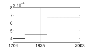
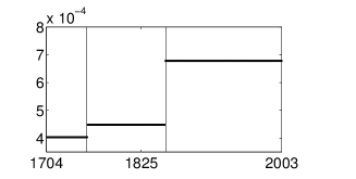
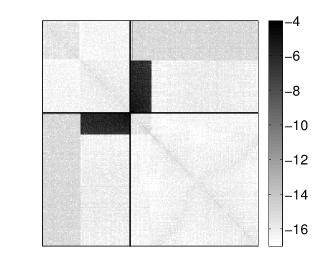
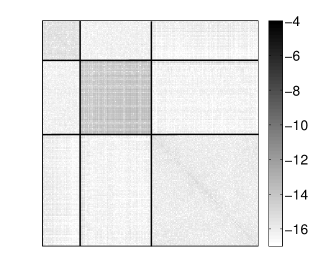
Figure 5: Computation of the eigenpairs corresponding to the $300$ largest eigenvalues $\lambda_{1704},\ldots,\lambda_{2003}$ with the subdivision point $\mu=\lambda_{1825}$ taken from a group of very close eigenvalues. The top plots show the eigenvalues and the subdivision points (vertical lines), the bottom plots give a pictorial visualization of the orthogonality $\left\lvert x_{i}^{H}Bx_{l}\right\rvert$, $i\not=l$.

5 Conclusions

We expounded the close connection between FEAST algorithm and the well-established Rayleigh–Ritz method for computing selected eigenpairs of a generalized eigenproblem. Starting from the mathematical foundation of this connection, we identified aspects of the solver that might play a critical role for its accuracy and reliability. Specifically, we discussed the choice of starting basis and stopping criterion, and the relation between the accuracy of the solutions of the linear systems internal to FEAST and the resulting eigenpairs; we also investigated the use of FEAST for computing a large portion or even the entire eigenspectrum. Through numerical examples we illustrated how each of these aspects might affect the robustness of the algorithm or diminish the quality of the computed eigensystem.

While we hinted at possible improvements for several of the existing issues, some questions remain open and are the subject of further research. For instance, a mechanism is needed to overcome the problem of having to specify both the boundaries of the search interval and the number of eigenvalues expected. Additionally, it would be desirable to have a flag assessing whether all the eigenpairs in the search interval have been found. Finally, orthogonality across multiple intervals should be guaranteed.

In summary, our findings suggest that at the moment FEAST is a promising eigensolver for a certain class of problems, i. e., when a small portion of the spectrum is sought and knowledge of the eigenvalue distribution is available. On the other hand, we believe it is still not yet competitive as a robust “black box”, general-purpose solver.

References

- [1] E. Polizzi, Density-matrix-based algorithm for solving eigenvalue problems, Phys. Rev. B 79 (2009) 115112.
- [2] T. Sakurai, H. Sugiura, A projection method for generalized eigenvalue problems using numerical integration, J. Comput. Appl. Math. 159 (2003) 119–128.
- [3] T. Sakurai, Y. Kodaki, H. Tadano, D. Takahashi, M. Sato, U. Nagashima, A parallel method for large sparse generalized eigenvalue problems using a GridRPC system, Future Generation Computer Systems 24 (2008) 613–619.
- [4] T. Ikegami, T. Sakurai, U. Nagashima, A filter diagonalization for generalized eigenvalue problems based on the Sakurai-Sugiura projection method, J. Comput. Appl. Math. 233 (2010) 1927–1936.
- [5] R. B. Lehoucq, D. C. Sorensen, C. Yang, ARPACK Users’ Guide, SIAM, Philadelphia, 1998.
- [6] K. Wu, H. Simon, Thick-restart Lanczos method for large symmetric eigenvalue problems, SIAM J. Matrix Anal. Appl. 22 (2000) 602–616.
- [7] Y. Zhou, Y. Saad, M. L. Tiago, J. R. Chelikowsky, Self-consistent-field calculations using Chebyshev-filtered subspace iteration, J. Comput. Phys. 219 (2006) 172–184.
- [8] Y. Zhou, A block Chebyshev–Davidson method with inner–outer restart for large eigenvalue problems, J. Comput. Phys. 229 (2010) 9188–9200.
- [9] G. Stewart, Matrix Algorithms, Vol. II, Eigensystems, SIAM, Philadelphia, PA, 2001.
- [10] Y. Saad, Iterative Methods for Sparse Linear Systems, 2nd Edition, SIAM, Philadelphia, PA, 2003.
- [11] P. J. Davis, P. Rabinowitz, Methods of Numerical Integration, 2nd Edition, Academic Press, Orlando, FL, 1984.
- [12] G. H. Golub, C. F. Van Loan, Matrix Computations, 3rd Edition, Johns Hopkins University Press, Baltimore, MD, 1996.
- [13] B. N. Parlett, The Symmetric Eigenvalue Problem, Classics Edition, Vol. 20 of Classics in Applied Mathematics, SIAM, Philadelphia, PA, 1998.
- [14] A. Frommer, U. Glässner, Restarted GMRES for shifted linear systems, SIAM J. Sci. Comput. 19 (1) (1998) 15–26.