Computational complexity and memory usage for multi-frontal direct solvers in structured mesh finite elements

Abstract

The multi-frontal direct solver is the state-of-the-art algorithm for the direct solution of sparse linear systems. This paper provides computational complexity and memory usage estimates for the application of the multi-frontal direct solver algorithm on linear systems resulting from B-spline-based isogeometric finite elements, where the mesh is a structured grid. Specifically we provide the estimates for systems resulting from $C^{p-1}$ polynomial B-spline spaces and compare them to those obtained using $C^{0}$ spaces.

1 Introduction

The main purpose of this paper is to explain in detail how one can derive estimates for computational complexity and memory usage of the multifrontal direct solver algorithm as applied to B-spline-based [1, 2] isogeometric finite elements [3, 4]. In this paper we generalize results already published for $C^{0}$ finite element spaces for the multi-frontal solver [5, 6].

The restriction of this work to structured grid meshes is due to the target application being B-spline-based isogeometric finite elements. Isogeometric analysis is a relatively new method that has been the subject of much work in recent years. While at its core it is spline-based isoparametric finite element analysis, the spaces used possess unique refinement strategies that form spaces that are supersets of conventional finite elements. The mesh in B-spline-based isogeometric analysis is always a structured grid of uniform polynomial order. This simplification allows for specialized complexity and memory usage estimates to be developed for these spaces when the direct solver is the multi-frontal solver.

The higher continuous basis is known to approximate smooth functions (e.g. solutions to PDEs) with orders of magnitude fewer degrees of freedom than their $C^{0}$ counterparts. While this is a promising result, the linear systems resulting from inner products of the higher continuous basis functions are also orders of magnitude more expensive to solve. This is something we have addressed in a previous paper [7]. In this paper we explain the derivation of the estimates in more detail and extend them to all spatial dimensions.

First we explain the concepts behind the multifrontal direct solver algorithm and highlight why the algorithm is well-suited to handle linear systems resulting from traditional $C^{0}$ finite elements spaces. We emphasize the perspective that the algorithm may be viewed as early $LU$-factorization. Second we evaluate computational complexity of a single level of the multifrontal algorithm. Last we generalize the single level result to all levels and provide estimates for $C^{0}$ and $C^{p-1}$ B-splines spaces.

2 Multi-frontal direct solver algorithm

The state of the art direct solver for sparse linear systems is the multi-frontal solver proposed by [8, 9]. It is the generalization of the frontal solver algorithm proposed by [10]. Note that while in [10], the original idea was developed for finite elements, the generalization applies to general sparse linear systems.

The key observation in the algorithm is that $LU$-factorization may be started during assembly on portions of the linear system that are fully assembled on a local level. The general algorithm first examines the matrix sparsity pattern to locate fully assembled matrix blocks which are loosely connected to the remaining part of the matrix. When used with finite elements, these blocks may be automatically determined using what is known about the support of the basis functions.

In the context of finite elements, the multifrontal direct solver algorithm works in the following manner. We create the elemental matrices using standard finite element procedures. In the direct solver terminology, these elemental matrices are known as frontal matrices. The element matrices are typically assembled into a global matrix, where contributions from shared degrees of freedom with other elements are combined. However, depending on the topology and order of the finite elements, there are degrees of freedom which at the element level are fully assembled. For efficiency, these fully assembled degrees of freedom are eliminted in terms of the partially assembled ones at the element level, that is, at the frontal level. Since this procedure can be repeated concurrently at each element, it is usually known as multi-frontal. Particularizing this idea to finite elements, we will start with an example of a two element finite element mesh in any spatial dimension.

2.1 Single level example: two element mesh

Consider the partitioning of the elemental matrices in equation (1). We reorder the elemental matrices by first listing those degrees of freedom that are fully assembled on the element level, $x_{e}$, followed by those that are shared with other elements, $y_{e}$, where subscript $e$ refers to the element number. Thus the element matrix can be blocked accordingly to represent interactions between fully assembled degrees of freedom and those shared with other elements. Note that $A_{e}$ represents the block of interactions which are fully assembled at the element level, blocks $B_{e}$ and $C_{e}$ represent the interactions of fully assembled and shared degrees of freedom, and block $D_{e}$ represents interactions of shared degrees of freedom. Particularizing this for the two element mesh, we obtain

$$\begin{bmatrix}A_{1}&B_{1}\\ C_{1}&D_{1}\end{bmatrix}\cdot\begin{bmatrix}x_{1}\\ y_{1}\end{bmatrix}=\begin{bmatrix}f_{1}\\ g_{1}\end{bmatrix},\hskip 36.135pt\begin{bmatrix}A_{2}&B_{2}\\ C_{2}&D_{2}\end{bmatrix}\cdot\begin{bmatrix}x_{2}\\ y_{2}\end{bmatrix}=\begin{bmatrix}f_{2}\\ g_{2}\end{bmatrix}$$ (1)

Because the block $A_{e}$ is fully assembled, we may begin the $LU$-factorization early and at the element level. Thus for each element, we can multiply the top row by $C_{e}A_{e}^{-1}$ and subtract from the bottom row,

$$\begin{bmatrix}A_{e}&B_{e}\\ 0&D_{e}-C_{e}A_{e}^{-1}B_{e}\end{bmatrix}\cdot\begin{bmatrix}x_{e}\\ y_{e}\end{bmatrix}=\begin{bmatrix}f_{e}\\ g_{e}-C_{e}A_{e}^{-1}B_{e}\end{bmatrix}$$ (2)

Then, for each element $e=1,2$, the block matrix $D_{e}-C_{e}A_{e}^{-1}B_{e}$ and the vector $g_{e}-C_{e}A_{e}^{-1}B_{e}$ is assembled. After the contributions from both elements are assembled, we can solve for $y$. Once $y$ is computed, we can resort to backward substitution at the element level to compute $x_{e}$.

2.2 Multilevel example: eight element mesh in three dimensions

The procedure can be recursively generalized into multiple levels. For example, the procedure for an eight element mesh is shown in figure 1. The elimination proceeds as follows:

1. Perform the local elimination of fully assembled degrees of freedom in each element as described in section 2.1. Note that the degrees of freedom eliminated, if any, are those which have support only on the element, the so-called bubble functions.

2. Pair the eight elements into any 4 clusters where the pairs of elements share a common face. To these frontal matrices, we apply the algorithm again, that is, we eliminate the fully assembled degrees of freedom in terms of the remaining degrees of freedom shared with other elements. At this level, the degrees of freedom eliminated are those with support on the shared face.

3. At the next level, we pair the four element clusters again into two which share a common interface. The recursive elimination procedure is applied at this level and repeated until we obtain a single cluster whose degrees of freedom are fully assembled (the top level in figure 1).

The connectivity graph describing the order of elimination and clustering is called the elimination tree. At this point, with the solution to the fully assembled system, we can move down the elimintation tree, using backward substitution to recover the remaining unknown degrees of freedom (those that were fully assembled at each elimination level).

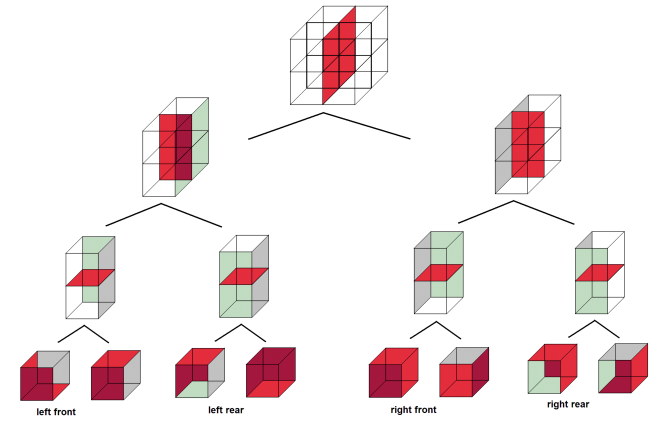
Figure 1: The four levels of the elimination tree for a cube-shaped mesh with eight finite elements

3 Computational complexity and memory usage

Now we look at complexity comparing higher-continuous B-spline spaces to their $C^{0}$ counterparts. For simplicity we will only consider spaces which are $C^{p-1}$ continuous, that is, spaces which have $p-1$ continuous derivatives across element interfaces, where $p$ refers to the polynomial order. Numerical tests indicate that these spaces form limiting cases in the performance of the direct solver algorithm.

The examples in the previous section come from $C^{0}$ finite element spaces. In these examples, $(p-1)^{d}$ degrees of freedom may be eliminated at the first level, where $d$ refers to the spatial dimension. For $C^{p-1}$ spaces, the supports of the basis functions spread into multiple elements and thus no degrees of freedom may be eliminated at the element level. To be able to eliminate a degree of freedom, we will cluster $p+1$ elements in each spatial dimension together and use this on the first level for $C^{p-1}$ spaces. This is the smallest grouping that can be obtained where a degree of freedom is fully assembled.

In the remaining portion of this section we will develop the estimates for complexity and memory usage. Computational complexity will be estimated by counting floating point operations (FLOPS) and the memory usage will we counted as the bytes needed to store the $LU$ factorization at each level of the elimination tree. The main building block of the algorithm is the early $LU$-factorization, also known as the Schur complement or static condensation. We will first develop the cost of the Schur complement, and then proceed to apply this to the full algorithm.

3.1 Cost of the Schur complement

In order to estimate the FLOPS and memory required to perform the above partial $LU$ factorization, we will count operations and memory used in forming the Schur complement, as shown in equation (2). We denote the dimension of the square matrix $A$ by $q$. We denote the number of columns in $B$ and rows in $C$ as $r$, where $r$ is an assumed a constant. Then, we have:

FLOPS = $${\cal O}(q^{3}+q^{2}r+qr^{2})={\cal O}(q^{3}+qr^{2})$$

Memory=

(3)

The FLOPS estimate is obtained by counting the operations needed to find the $LU$ factors of $A$, $\mathcal{O}(q^{3})$. To this we add the FLOPS required to perform $r$ back-substitutions to form $A^{-1}B$, $\mathcal{O}(rq^{2})$. Finally, we add the cost of matrix multiplication of $C$ to $A^{-1}B$, $\mathcal{O}(qr^{2})$. The memory estimate is obtained by adding the memory needed to store the $LU$ factors of the matrix $A$, $\mathcal{O}(q^{2})$, to that required to store $A^{-1}B$ and $CA^{-1}$, $\mathcal{O}(rq)$.

In the above memory estimate, we are only concerned with the space required to store $L$ and $U$, since it is well-known that the cost of storing original matrix is always smaller or equal than the memory required to store factors $L$ and $U$. In particular, we have not included the memory required to store the Schur complement, since this is replaced in the next steps of $LU$ factorization by additional Schur complement operations.

3.2 Cost of the multi-frontal solver

We divide our computational domain in $N_{c}$ clusters of elements. For the $C^{0}$ case, each cluster is simply an element, while for $C^{p-1}$, each cluster is a set of $p+1$ consecutive elements in each spatial dimension. We assume for simplicity that the number of clusters in our computational domain is $(2^{d})^{s}$, where $s$ is a positive integer which represents the number of levels of the multi-frontal algorithm. Notice that even if this assumption is not verified, the final result still holds true provided that the number of degrees of freedom is sufficiently large.

The multi-frontal direct solver algorithm is summarized in algorithm  1. The FLOPS and memory required by algorithm 1 can be expressed as

$$\sum_{i=0}^{s-1}N_{c}(i)S(i)$$ (4)

where $S(i)$ is the cost (either FLOPS or memory) of performing each Schur complement at the $i^{th}$ level. Using the notation of the previous subsection on the Schur complement, we define $q=q(i)$ as the number of interior unknowns of each cluster at the $i^{th}$ step, and $r=r(i)$ as the number of interacting unknowns at the $i^{th}$ step. We construct estimates for these numbers and summarize them in table 1.

Algorithm 1 Multi-Frontal Algorithm

1:for $i=0\mbox{ to }s-1$ do

2:     $N_{c}=N_{c}(i)=(2^{d})^{s-i}$

3:     if $i=0$ then

4:         Define $N_{c}(0)$ clusters

5:     else

6:         Join the old $N_{c}(i-1)$ clusters

7:         Eliminate interior degrees of freedom

8:         Define $N_{c}(i)$ new clusters

9:     end if

10:end for

Table 1: Number of interior ($q$) and interacting ($r$) unknowns at each level $i$ of the multi-frontal solver.

		$q(0)$	$r(0)$		$q(i),\ i\neq 0$	$r(i),\ i\neq 0$
$C^{0}$		${\cal O}(p^{d})$	${\cal O}(p^{d-1})$		${\cal O}(2^{(d-1)i}p^{d-1})$	${\cal O}(2^{(d-1)i}p^{d-1})$
$C^{p-1}$		${\cal O}(1)$	${\cal O}(p^{d})$		${\cal O}(2^{(d-1)i}p^{d})$	${\cal O}(2^{(d-1)i}p^{d})$

Let $N$ be the total number of unknowns in the original system. We use the results from table 1 with the FLOPS and memory estimates in equation (3) to develop table 2. This table describes the cost in FLOPS and memory of each level of the multi-frontal algorithm.

Table 2: FLOPS and memory estimates at each level $i$ of the multi-frontal solver.

		FLOPS	Memory		FLOPS	Memory
		S(0)	S(0)		S(i) , $i\neq 0$	S(i) , $i\neq 0$
$C^{0}$		${\cal O}(p^{9})$	${\cal O}(p^{6})$		${\cal O}(2^{6i}p^{6})$	${\cal O}(2^{4i}p^{6})$
$C^{p-1}$		${\cal O}(p^{6})$	${\cal O}(p^{3})$		${\cal O}(2^{6i}p^{9})$	${\cal O}(2^{4i}p^{6})$

Finally we use equation (4) and table 2 to specialize estimates for $C^{0}$ and $C^{p-1}$ B-splines in one to three spatial dimensions.

Estimates for 1D $C^{0}$ B-splines

FLOPS = $$2^{s}p^{3}+\sum_{i=1}^{s-1}2^{s-i}={\cal O}(2^{s}p^{3})={\cal O}(N_{p}p^{3})={\cal O}(Np^{2})$$

Memory =

Estimates for 1D $C^{p-1}$ B-splines

FLOPS = $$2^{s}p^{2}+\sum_{i=1}^{s-1}2^{s-i}p^{3}={\cal O}(2^{s}p^{3})={\cal O}(N_{p}p^{3})={\cal O}(Np^{2})$$,

Memory = .

Estimates for 2D $C^{0}$ B-splines

FLOPS = $$2^{2s}p^{6}+\sum_{i=1}^{s-1}2^{2(s-i)}2^{3i}p^{3}={\cal O}(2^{2s}p^{6}+2^{3s}p^{3})=$$

Memory =

Estimates for 2D $C^{p-1}$ B-splines

FLOPS = $$2^{2s}p^{4}+\sum_{i=1}^{s-1}2^{2(s-i)}2^{3i}p^{6}={\cal O}(2^{2s}p^{4}+2^{3s}p^{6})=$$

Memory =

Estimates for 3D $C^{0}$ B-splines

FLOPS = $$2^{3s}p^{9}+\sum_{i=1}^{s-1}2^{3(s-i)}2^{6i}p^{6}={\cal O}(2^{3s}p^{9}+2^{6s}p^{6})=$$

Memory =

Estimates for 3D $C^{p-1}$ B-splines

FLOPS = $$2^{3s}p^{6}+\sum_{i=1}^{s-1}2^{3(s-i)}2^{6i}p^{9}={\cal O}(2^{3s}p^{6}+2^{6s}p^{9})=$$

Memory =

4 Numerical Results

To test the validity of these estimates, we compute solutions to the Laplace equation in three spatial dimensions on the unit cube

$$\begin{cases}-\nabla\cdot(\nabla u)=0&\ \ \ \text{on }\Omega\\ u=0&\ \ \ \text{on }\Gamma_{D0}\\ u=1&\ \ \ \text{on }\Gamma_{D1}\\ (\nabla u)\cdot\mathbf{n}=0&\ \ \ \text{on }\Gamma_{N}\end{cases}$$ (5)

where $\Omega=[0,1]^{3}$, $\Gamma_{D0}=(:,:,0)$, $\Gamma_{D1}=(:,:,1)$, and $\Gamma_{N}=(0,:,:)\cup(1,:,:)\cup(:,0,:)\cup(:,1,0)$.

All computational experiments have been performed on a workstation with two quad-core Xeon X5550 processors and 24 Gb of memory running Fedora 11. The model problem was implemented using PETSc [11, 12] data structures. We used the MUMPS [13, 14] implementation of the multi-frontal algorithm, with METIS [15] ordering (nested dissection). We interfaced to MUMPS through PETSc, with the option to solve an asymmetric system. Note that only one core was used in these numerical experiments.

For all numerical results, we relate the FLOPS estimates to the computational time measured for the solution of the linear system. The memory estimates we relate to the number of nonzero entries in the $LU$ factors. We report the memory required to store an integer and a double precision number for each nonzero entry. Note that this is a conservative quantification of memory usage. In general, solvers will require the use of additional memory. However, we chose to report the memory required to store the $LU$ factors as it is most closely related to the estimates derived in the previous section.

We tested the estimates by solving the model problem for a linear system containing 100,000 degrees of freedom for both $C^{0}$ and $C^{p-1}$ spaces. This was accomplished by using different numbers of elements. Note that while this will affect assembly time, this is not included here in the time reported.

The numeric results of this test are shown in figure 2. We show computational time and memory usage for the $C^{0}$ spaces. The solid line shown in a statistical best fit of the data to the estimate. The excellent agreement between the estimates and the real data supports the accuracy of the estimates.

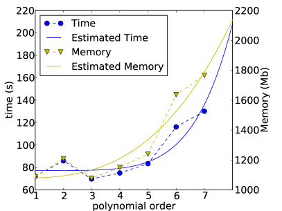
(a) $C^{0}$ B-spline spaces

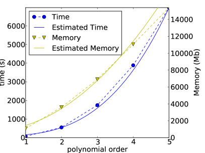
(b) $C^{p-1}$ B-spline spaces

Figure 2: Time and memory for 100,000 degrees of freedom systems along with estimates

5 Conclusions

In this paper, we derive estimates for the computational complexity and memory usage of the multifrontal direct solver algorithm applied to finite elements, where the mesh is a structured grid. This restriction is with a view to forming estimates for higher continuous spaces, $C^{p-1}$ B-spline spaces. We present numerical results to support the validity of these estimates.

We observe that the estimates for 1D, 2D, and 3D are essentially different. This is because of the structure of what can be eliminated at each level. Although in 1D the number of FLOPS is linear with respect the number of unknowns $N$, this case is not interesting. We note that for $C^{0}$ spaces in two and three spatial dimensions, the number of FLOPS is independent of $p$ if the number of unknowns $N$ is large enough. Therefore, under the assumption that $N$ is large enough, an adaptive algorithm should select refinements based exclusively on the maximum decrease of error per added unknown, independently of wether the refinement takes place on $h$ or $p$, where $h$ here refers to the support of the basis function. This efficiency is exploited in the adaptive algorithms used in $hp$-finite elements [16].

For 2D and 3D, the number of FLOPS of the $C^{p-1}$ spaces is $p^{3}$ times more expensive than the $C^{0}$ spaces, provided $N$ is large enough. Thus, an adaptive algorithm for isogeometric analysis should not be based exclusively on the maximum decrease of the error per added unknown. It would need to incorporate a special treatment of the cost of each added unknown depending upon the type of refinement.

6 Acknowledgements

DP has been partially supported by the Spanish Ministry of Sciences and Innovation Grant MTM2010-16511. MRP has been partially supported by the Polish MNiSW grant no. NN 519 405737 and NN519 447 739.

References

- [1] G. Farin, Curves and Surfaces for CAGD: A Practical Guide, 5th Edition, Morgan Kaufmann, 2002.
- [2] L. Piegl, W. Tiller, The NURBS Book, Monographs in Visual Communication, Springer, New York, 1995.
- [3] T. J. R. Hughes, J. Cottrell, Y. Bazilevs, Isogeometric analysis: CAD, finite elements, NURBS, exact geometry and mesh refinement, Computer Methods in Applied Mechanics and Engineering 194 (2005) 4135–4195.
- [4] J. Cottrell, A. Reali, Y. Bazilevs, T. J. R. Hughes, Isogeometric analysis of structural vibrations., Computer Methods in Applied Mechanics and Engineering 195 (41-43) (2006) 5257.
-
[5]
V. M. Calo, N. O. Collier, D. Pardo, M. R. Paszynski,