Gradient-based estimation of Manning’s friction coefficient from noisy data

Abstract

We study the numerical recovery of Manning’s roughness coefficient for the diffusive wave approximation of the shallow water equation. We describe a conjugate gradient method for the numerical inversion. Numerical results for one-dimensional model are presented to illustrate the feasibility of the approach. Also we provide a proof of the differentiability of the weak form with respect to the coefficient as well as the continuity and boundedness of the linearized operator under reasonable assumptions using the maximal parabolic regularity theory.
Keywords: diffusive shallow water equation, parameter identification

1 Introduction

The diffusive wave approximation (DSW) of the shallow water equations (SWE) is often used to model overland flows such as floods, dam breaks, and flows through vegetated areas [20, 12, 8]. The SWE result from the full Navier-Stokes system with the assumption that the vertical momentum scales are small relative to those of the horizontal momentum. This assumption reduces the vertical momentum equation to a hydrostatic pressure relation, which is integrated in the vertical direction to arrive at a two-dimensional system known as the SWE. The DSW further simplifies the SWE by assuming that the horizontal momentum can be linked to the water height by an empirical formula, such as Manning’s formula (also known as Gauckler-Manning formula [9]) [4, 21]. The DSW is a scalar parabolic equation which resembles nonlinear diffusion.

The DSW gives rise to the following initial/boundary value problem for the water height $u$

$$\left\{\begin{array}[]{ll}\dfrac{\partial u}{\partial t}-\nabla\cdot\left(k\left(u,\nabla u\right)\nabla u\right)=f&\mbox{in }\Omega\times(0,T]\\ u=u_{0}&\mbox{on }\Omega\times\{t=0\}\\ \left(k\left(u,\nabla u\right)\nabla u\right)\cdot n=h&\mbox{on }\Gamma_{N}\times(0,T]\\ u=g&\mbox{on }\Gamma_{D}\times(0,T]\end{array}\right.$$ (1)

where $\Omega$ is an open bounded domain in $\mathbb{R}^{d}\ (d=1,2)$, and $\Gamma_{N}$ and $\Gamma_{D}$ are disjoint subsets of the boundary $\Gamma=\partial\Omega$ such that $\Gamma=\Gamma_{N}\cup\Gamma_{D}$. The forcing function (e.g., rainfall acting as a source or infiltration acting as a sink) $f:\Omega\times(0,T]\rightarrow\mathbb{R}$, the initial condition $u_{0}:\Omega\rightarrow\mathbb{R}$, and the Neumann and Dirichlet boundary conditions $h:\Gamma_{N}\times(0,T]\rightarrow\mathbb{R}$ and $g:\Gamma_{D}\times(0,T]\rightarrow\mathbb{R}$ are given. The diffusion coefficient $k(u,\nabla u)$ is given by

$$k(u,\nabla u)=\dfrac{1}{c_{f}}\dfrac{\left(u-z\right)^{\alpha}}{\left|\nabla{}u\right|^{1-\gamma}}=d_{f}\dfrac{\left(u-z\right)^{\alpha}}{\left|\nabla u\right|^{1-\gamma}},$$

where $z:\overline{\Omega}:\rightarrow\mathbb{R}^{+}$ is a nonnegative time-independent function that represents the bathymetric or topographic measurements available for the region under analysis. The parameters $\gamma$ and $\alpha$ satisfy $0<\gamma\leq 1$ and $1<\alpha<2$. Following Manning’s formula [17], we set these parameters to $\gamma=\frac{1}{2}$ and $\alpha=\frac{5}{3}$. The function $c_{f}$ (or equivalently $d_{f}=\frac{1}{c_{f}}$) represents Manning’s roughness coefficient, also known as the friction coefficient. The typical values are available in the literature [3, 19]. We refer to [2, 17] for recent mathematical analysis and to [17, 5] for efficient numerical algorithms.

In practice, the Manning coefficient $c_{f}$ is an empirically derived coefficient, and historically it was expected to be constant and a function of the roughness only. It is now widely accepted that the values of the coefficients $c_{f}$ are only constant within some range of flow rates, and depends strongly on many factors, including surface roughness, sinuosity and flow reach. The presence of multiple influencing factors renders a direct measurement of the coefficient values less reliable and the use of a single-valued coefficient also greatly constrains the practical utility of the DSW model to faithfully capture important physical features of real open channel flows, for which a spatially-varying coefficient is necessary due to distinct physical characteristics of different regions.

In this study, we propose to estimate the distributed Manning coefficient directly from water height measurements using inversion techniques, that is, formulating an inverse problem for identifying the friction coefficient $c_{f}$ from measurements of the water-height acquired by sensors and infrared imaging. In comparison with direct measurement, the proposed approach does not require a knowledge of the physical properties of the overland environment, which might be difficult to directly incorporate, and moreover, can naturally handle spatially varying coefficients. Therefore, a reliable and efficient estimate of this coefficient is expected to greatly broaden the scope of the DSW model and to facilitate real-time simulation of the flow, which is of immense significance in a number of applications, for example flood prediction and flood hazard assessment. The goal of the present study is to propose an inversion algorithm and demonstrate its feasibility on simulation data for one-dimensional models.

We briefly comment on relevant studies on the inverse problem. Due to its conceived practical significance, it has received some attention in the literature [6, 7]. For example, Ding et al [6] estimated the Manning’s coefficient in the SWE within the variational framework using the limited memory quasi-Newton method, and compared its performance with several other optimization algorithms. However, these works have considered only the situation of recovering a few parameters (with a maximum three), instead of estimating a distributed Manning’s coefficient like here. If the number of unknowns is small, the ill-posed nature of the problem does not evidence directly. Therefore, the present work represents a nontrivial step towards the important task of estimating distributed Manning’s roughness coefficients.

2 Linearization of the forward map

In this section we describe the linearization of the forward map $F:d_{f}\rightarrow u(d_{f})$, where $u(d_{f})$ denotes the solution to system (1). The linearization is required for solving the forward problem (with a predictor-corrector method) and the inverse problem (adjoint and sensitivity problems, see Section 3). Therefore, its derivation is of independent interest. In order to make the presentation accessible, we choose to derive the derivative operator informally. A rigorous derivation can be found in Appendix A.

The bilinear form of problem (1) is

$$B(u,w) =\int_{\Omega}u_{t}wdx+\int_{\Omega}k(u,\nabla u)\nabla u\cdot\nabla wdx$$

$$=\left(u_{t},w\right)+\left(k(u,\nabla u)\nabla u,\nabla w\right),$$

and the linear form is

$$\ell(w)=\int_{\Omega}fwdx+\int_{\Gamma_{N}}hwds=(f,w)+(h,w)_{\Gamma_{N}}.$$

The weak formulation of the problem reads: For almost all $t\in(0,T]$, find $u$ with the given Dirichlet boundary condition and initial data $u(0)=u_{0}$ such that

$$B(u,w)=\ell(w)\quad\forall w\in V,$$

where $V$ is an appropriate function space [17].

We shall seek the Gâteaux derivative of the bilinear form $B$ at $u$, that is, $\frac{d}{d\epsilon}B(u+\epsilon v,w)|_{\epsilon=0}$. We aim at deriving an explicit formula to facilitate further developments. We proceed as follows. It follows from the product rule for differentiation that

$$\left.\dfrac{\partial B(u+\epsilon v,w)}{\partial\epsilon}\right|_{\epsilon=0}= \dfrac{\partial}{\partial\epsilon}\left.\left[\left(u_{t}+\epsilon v_{t},w\right)+\left(d_{f}\dfrac{\left[\left(u+\epsilon v\right)-z\right]^{\alpha}}{\left|\nabla u+\epsilon\nabla v\right|^{1-\gamma}}\left(\nabla u+\epsilon\nabla v\right),\nabla w\right)\right]\right|_{\epsilon=0}$$

$$= \left(v_{t},w\right)+\left(d_{f}\frac{(u-z)^{\alpha}}{\left|\nabla u\right|^{1-\gamma}}\nabla v,\nabla w\right)+I+II,$$

where the terms $I$ and $II$ are respectively given by

$$I =\left.\left(d_{f}\,\dfrac{\partial[u+\epsilon v-z]^{\alpha}}{\partial\epsilon}\frac{\nabla u+\epsilon\nabla v}{|\nabla u+\epsilon\nabla v|^{1-\gamma}},\nabla w\right)\right|_{\epsilon=0}=\left(d_{f}\,\alpha\,\dfrac{\left(u-z\right)^{\alpha-1}}{\left|\nabla u\right|^{1-\gamma}}\,v\nabla u,\nabla w\right),$$

and

$$II =\left.\left(d_{f}[u+\epsilon v-z]^{\alpha}\frac{\partial|\nabla u+\epsilon\nabla v|^{\gamma-1}}{\partial\epsilon}\left(\nabla u+\epsilon\nabla v\right),\nabla w\right)\right|_{\epsilon=0}$$

$$=\left(d_{f}\,\left(u-z\right)^{\alpha}\,(\gamma-1)\left|\nabla u\right|^{\gamma-2}\dfrac{\nabla u}{|\nabla u|}\cdot\nabla v\,\nabla u,\nabla w\right)$$

$$=\left(d_{f}\,(\gamma-1)\,\dfrac{\left(u-z\right)^{\alpha}}{\left|\nabla u\right|^{3-\gamma}}\nabla u\cdot\nabla v\,\nabla u,\nabla w\right).$$

Here the second line follows from the relation $|\nabla u|=\sqrt{\nabla u\cdot\nabla u}=(\nabla u\cdot\nabla u)^{\frac{1}{2}}$ that implies

$$\left.\dfrac{\partial|\nabla u+\epsilon\nabla v|}{\partial\epsilon}\right|_{\epsilon=0} =\dfrac{1}{2}\left(\left(\nabla u+\epsilon\nabla v\right)\cdot\left(\nabla u+\epsilon\nabla v\right)\right)^{-\frac{1}{2}}\,2(\nabla u+\epsilon\nabla v)\cdot\nabla v|_{\epsilon=0}=\dfrac{\nabla u\cdot\nabla v}{|\nabla u|}.$$

Consequently, by combining all these identities, we arrive at the following formula

$$\left.\dfrac{\partial B\left(u+\epsilon v,w\right)}{\partial\epsilon}\right|_{\epsilon=0}= \left(v_{t},w\right)+\left(d_{f}\dfrac{(u-z)^{\alpha}}{|\nabla u|^{1-\gamma}}\nabla v,\nabla w\right)$$

$$\quad+\left(d_{f}\alpha\frac{(u-z)^{\alpha-1}}{|\nabla u|^{1-\gamma}}\,v\,\nabla u,\nabla w\right)$$

$$\quad+\left(d_{f}(\gamma-1)\frac{(u-z)^{\alpha}}{|\nabla u|^{1-\gamma}}\,\dfrac{\nabla u}{|\nabla u|}\cdot\nabla v\,\dfrac{\nabla u}{|\nabla u|},\nabla w\right)$$

$$= \left(v_{t},w\right)+\left(k(u,\nabla u)\left(I-\left(1-\gamma\right)\tilde{\eta}\otimes\tilde{\eta}\right)\cdot\nabla v,\nabla w\right)$$

$$\quad+\left(k(u,\nabla u)\,\frac{\alpha}{(u-z)}\,v\,\nabla u,\nabla w\right)$$

where $I$ is the identity operator and the vector field $\tilde{\eta}=\tfrac{\nabla u}{|\nabla u|}$ is the normalized gradient vector field. The matrix-valued function $\tilde{\eta}\otimes\tilde{\eta}$ represents a projection operator onto the gradient direction $\tilde{\eta}$. Hence, the structure of the second term indicates that, for the linearized problem, the diffusion along the gradient direction is attenuated by $1-\gamma$, whereas the tangential component is not affected. To simplify notation we denote this attenuated diffusion tensor as

$$k_{\eta\eta}(u,\nabla u)=k(u,\nabla u)\left(I-\left(1-\gamma\right)\tilde{\eta}\otimes\tilde{\eta}\right).$$

Meanwhile, the linearized problem has a convection term (the third term), as a consequence of the nonlinear term involving $u$. These structural terms relate to the underlying physics of the model.

It follows directly from the definition of the Gâteaux derivative, i.e., which is denoted by $v=u^{\prime}(d_{f})d\in V$ and characterizes the perturbation of $u(d_{f})$ caused by a small perturbation of the coefficient $d_{f}$ in the direction $d$ that it (in weak formulation) satisfies

$$\left(v_{t},w\right) +\left(k_{\eta\eta}(u,\nabla u)\cdot\nabla v,\nabla w\right)+\left(\dfrac{\alpha\,k(u,\nabla u)}{(u-z)}\,v\,\nabla u,\nabla w\right)=-\left(d\dfrac{(u-z)^{\alpha}}{\left|\nabla u\right|^{1-\gamma}}\nabla u,\nabla w\right)$$

and the initial condition is $v(0)=0$, since the initial data is not affected by a perturbation of the friction coefficient.

3 Inversion algorithm

Now we turn to the inverse problem of reconstructing the coefficient $d_{f}$ from the measurements of water heights. As a general rule, the inverse problem is ill-posed in the sense that small perturbations in the data can lead to large changes in the solution. Hence we adopt a regularization strategy by incorporating a penalty term into the cost functional, following the pioneering idea of Tikhonov [18]. More precisely, we consider the following penalized misfit functional

$$J(d_{f})=\frac{1}{2}\int_{0}^{T}\int_{\Omega}(u(d_{f})-g)^{2}dxdt+\frac{\delta}{2}\int_{\Omega}|\nabla d_{f}|^{2}dx,$$

where the scalar $\delta$ is the regularization parameter, and $g$ denotes the noisy measurements of the water height $u(d_{f})$. With minor modifications, the algorithm discussed below can also be applied to other measurements, for example, water height on the boundary or scattered in the domain. The term $\|\nabla d_{f}\|_{L^{2}(\Omega)}^{2}$ enforces smoothness on the sought-for coefficient, and thereby restores the numerical stability necessary for practical computations. To numerically minimize the functional, we adopt the conjugate gradient method. The method is of gradient descent type, and it only requires evaluating the gradient of the functional $J(d_{f})$ at each step. We note that the conjugate gradient method has been successfully applied to a wide variety of practical inverse problems, such as in heat transfer and mechanics; see for example, [1, 16] and references therein for details.

To derive a computationally efficient gradient formula, we first note that, given a (descent) direction $d$, the misfit term in the functional $J$ can be approximated using a Taylor expansion and ignoring higher order terms.

$$\frac{1}{2}\int_{0}^{T}\int_{\Omega}\left(u(d_{f}+d)-g\right)^{2} dxdt-\frac{1}{2}\int_{0}^{T}\int_{\Omega}\left(u(d_{f}\right)-g)^{2}dxdt=$$

$$= \frac{1}{2}\int_{0}^{T}\int_{\Omega}\left(u(d_{f}+d)-u(d_{f})\right)\left(u(d_{f}+d)-g+u(d_{f})-g\right)dxdt$$

$$\approx \int_{0}^{T}\int_{\Omega}u^{\prime}(d_{f})d\,\left(u(d_{f})-g\right)dxdt.$$

The approximation is reasonable if the magnitude of the direction $d$ is small.

The last formula can be further simplified with the help of the adjoint problem for $p$, which in weak form reads

$$\left(-p_{t},w\right)+\left(k_{\eta\eta}(u,\nabla u)\cdot\nabla p,\nabla w\right)+\left(\dfrac{\alpha\,k(u,\nabla u)}{(u-z)}\,\nabla u\cdot\nabla p,w\right)=\left(u(d_{f})-g,w\right)$$

together with the terminal condition $p(T)=0$. Recall the weak formulation of the sensitivity problem $v=u^{\prime}(d_{f})d$, that is,

$$\left(v_{t},w\right)+\left(k_{\eta\eta}(u,\nabla u)\cdot\nabla v,\nabla w\right)+\left(\dfrac{\alpha\,k(u,\nabla u)}{(u-z)}\,v\,\nabla u,\nabla w\right)=-\left(d\frac{(u-z)^{\alpha}}{|\nabla u|^{1-\gamma}}\nabla u,\nabla w\right),$$

together with the initial condition $v(0)=0$. Upon setting the test function $w=u^{\prime}(d_{f})\,d$ and $w=p$ in the weak formulations for $p$ and $u^{\prime}(d_{f})\,d$, respectively, we arrive at

$$\int_{0}^{T}\left(u(d_{f})-g,u^{\prime}(d_{f})\,d\right)dt=-\int_{0}^{T}\int_{\Omega} d\,\frac{(u-z)^{\alpha}}{|\nabla u|^{1-\gamma}}\nabla p\cdot\nabla udxdt-\int_{0}^{T}\frac{d}{dt}(p,u^{\prime}(d_{f})d)dt$$

$$=-\int_{0}^{T}\int_{\Omega} d\,\frac{(u-z)^{\alpha}}{|\nabla u|^{1-\gamma}}\nabla p\cdot\nabla udxdt,$$

where the last identity follows from the initial condition for $u^{\prime}(d_{f})\,d$ and terminal condition for $p$. This relation yields the following concise gradient formula of the functional $J(d_{f})$

$$J^{\prime}(d_{f})=-\int_{0}^{T}\frac{(u-z)^{\alpha}}{|\nabla u|^{1-\gamma}}\nabla p\cdot\nabla udt-\delta\Delta d_{f}.$$

We note that this gradient $J^{\prime}(d_{f})$ is inappropriate for updating the coefficient $d_{f}$ directly due to its lack of desired regularity. The consistent gradient of the functional with respect to $H^{1}(\Omega)$, denoted by $J_{s}^{\prime}(d_{f})$, can be calculated as

$$-\Delta J_{s}^{\prime}(d_{f})+J_{s}^{\prime}(d_{f})=J^{\prime}(d_{f})$$

with a homogeneous Neumann boundary condition.

Now we can give a complete description of the conjugate gradient method summarized in Algorithm 1. In the algorithm, one has the freedom to choose the conjugate coefficient $\beta_{k}$ and the step size $\theta_{k}$. There are several viable choices of the conjugate coefficient [11]. One popular choice is suggested by Fletcher-Reeves, which reads

$$\beta_{k-1}=\frac{\|J_{s}^{\prime}(d_{f}^{k})\|_{L^{2}(\Omega)}^{2}}{\|J_{s}^{\prime}(d_{f}^{k-1})\|_{L^{2}(\Omega)}^{2}}$$

with the convention $\beta_{0}=0$, and then update the conjugate direction $d_{k}$ with

$$d_{k}=J_{s}^{\prime}(d_{f}^{k})+\beta_{k-1}d_{k-1}.$$

Generally, the step size selection is of crucial importance for the performance of the algorithm. We have opted for the following simple rule. By means of a Taylor expansion of the objective function $J(d_{f}^{k}-\theta d_{k})$, with the forward solution $u(d_{f}^{k}-\theta d_{k})$ linearized around $d_{f}^{k}$, we arrive at the following approximate formula for determining an appropriate step size $\theta_{k}$

$$\theta_{k}=\frac{\langle r_{k},u^{\prime}(d_{f}^{k})d_{k}\rangle_{L^{2}(0,T;L^{2}(\Omega))}+\delta\langle\nabla d_{f}^{k},\nabla d_{k}\rangle_{L^{2}(\Omega)}}{\|u^{\prime}(d_{f}^{k})d_{k}\|_{L^{2}(0,T;L^{2}(\Omega))}^{2}+\delta\|\nabla d_{k}\|_{L^{2}(\Omega)}^{2}},$$

where $r_{k}=u(d_{f}^{k})-g$ denotes the misfit (residual). The step size $\theta_{k}$ is determined to enforce a reduction the functional value, that is, $J\left(d_{f}^{k}-\theta_{k}\,J_{s}^{\prime}(d_{f}^{k})\right)\leq J(d_{f}^{k})$. Our experience with other inverse problems indicates that this choice works reasonably well in practice [16]. Advanced step size selection rules, such as, Barzilai-Borwein rule with backtracking, maybe also be adopted to further enhance the performance. The algorithm terminates if the selected step size falls below $1.0\times 10^{-3}$. Overall, each step of the iteration invokes three forward solves: the (nonlinear) forward solve for computing the map $u(d_{f})$, the (linear) adjoint solve for calculating the adjoint $p(d_{f})$ and consequently the gradient $J^{\prime}(d_{f})$ and the (linear) sensitivity solve for selecting the step size $\theta$. The extra computational effort for computing the smoothed gradient $J_{s}^{\prime}(d_{f})$ is marginal compared with other steps due to its simple structure.

Algorithm 1 Conjugate gradient method.

1:  Set $k=0$ and choose initial guess $d_{f}^{0}$.

2:  repeat

3:     Solve direct problem with $d_{f}=d_{f}^{k}$, and determine residual $r_{k}=u(d_{f}^{k})-g$.

4:     Solve adjoint problem with right hand side $r_{k}$.

5:     Calculate gradient $J_{s}^{\prime}(d_{f}^{k})$, conjugate coefficient $\beta_{k}$, and direction $d_{k}$.

6:     Solve the sensitivity problem with direction $d=d_{k}$.

7:     Compute step length $\theta_{k}$ in conjugate direction $d_{k}$.

8:     Update coefficient $d_{f}^{k}=d_{f}^{k}-\theta_{k}d_{k}$.

9:     Increase $k$ by one.

10:  until A stopping criterion is satisfied.

11:  Output approximation $d_{f}$

4 Numerical experiments and discussions

Here we present some numerical results for one-dimensional examples to illustrate the feasibility of the proposed inversion technique. The forward problem is discretized using piecewise linear finite elements in space and the generalized-$\alpha$ method in time (detailed in Appendix B). The adjoint and sensitivity problems are both solved with the generalized-$\alpha$ method.

The spatial domain $\Omega=[-2,2]$, and the mesh size $h$ is $\frac{1}{4}$. The time interval is $\left[0,\frac{1}{2}\right]$, and the time step size is $\frac{1}{40}$. This mesh was used for both generating the exact data and used in the inversion step (i.e., adjoint problem and sensitivity problem). We note that we also experimented with using finer mesh for generating the exact data, and the reconstructions are identical. Also both the forward solution $u(d_{f})$ and the coefficient $d_{f}$ are represented in this mesh. The initial guess for the coefficient is $d_{f}=1$. The noisy data $g$ are generated pointwise as

$$g=u(d_{f}^{\dagger})+\varepsilon\max_{(x,t)\in\Omega\times[0,T]}\left(\left|u(d_{f}^{\dagger})\right|\right)\zeta,$$

where $\varepsilon$ is the relative noise level, and the random variable (noise) $\zeta$ follows a standard Gaussian distribution. The choice of the regularization parameter $\delta$ is crucial in any regularization strategies [18]. There have been intensive studies on its appropriate choice which have led to systematical and rigorous rules for choosing an appropriate value, see [15, 13] for recent progress. However, in this preliminary study, we have opted for the conventional trial-and-error approach.

We consider three examples: one with a smooth coefficient, and two with a discontinuous coefficient. First, we consider the recovery of a continuous coefficient.

Example 1.

The forward problem has a homogeneous Neumann boundary condition, and the initial condition $u_{0}$ is $u_{0}=-\frac{1}{4}x+\frac{3}{2}$. The exact coefficient is $d_{f}^{\dagger}(x)=1+\frac{1}{16}(x^{2}-4)^{2}$.

Figure 1(a) and Table 1 show the numerical results for Example 1, where $e$ is the relative error of an approximation $d_{f}$, defined as $e=\|d_{f}-d_{f}^{\dagger}\|_{L^{2}(\Omega)}/\|d_{f}^{\dagger}\|_{L^{2}(\Omega)}$. The reconstructions are in reasonable agreement with the exact coefficient $d_{f}^{\dagger}$ for up to $2\%$ noise in the data. Hence the proposed method is stable and accurate. We note that the approximation near the boundary seems less accurate compared to other regions. The error $e$ decreases as the noise level $\epsilon$ decreases to zero, see also Table 1. Overall, the convergence of the inversion algorithm is rather steady, see Figures 1(b) and (c). While the functional value $J(d_{f}^{k})$ decreases monotonically as the iteration proceeds, the convergence of the error $e$ exhibits a clear valley, indicating that a premature termination of the algorithm might result in sub-optimal reconstructions.

Table 1: Numerical results (error $e$) for different noise levels.

$\varepsilon$	$0\%$	$0.5\%$	$1\%$	$2\%$
Example 1	5.94e-3	2.00e-2	2.90e-2	4.52e-2
Example 2	4.49e-2	6.41e-2	7.49e-2	9.99e-2
Example 3	4.05e-2	5.15e-2	5.94e-2	9.42e-2

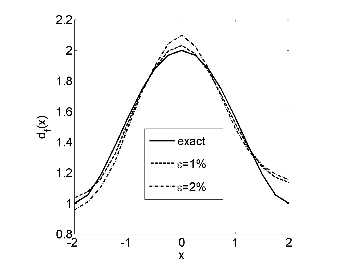
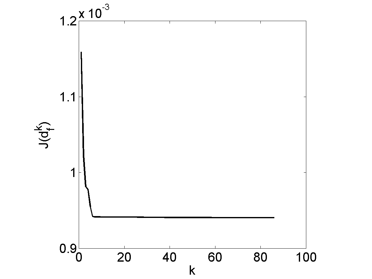
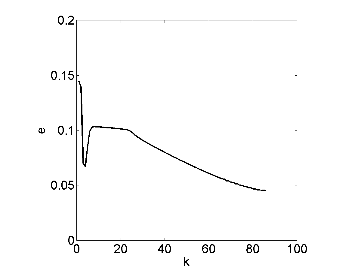
(a) reconstructions	(b) functional value $J(d_{f}^{k})$	(c) error $e$

Figure 1: Numerical results for Example 1. Here the convergence of Algorithm 1 is for $\varepsilon=2\%$ noise.

Then we consider the recovery of a discontinuous coefficient.

Example 2.

The boundary condition and initial condition of the problem are identical to those in Example 1. The exact coefficient is $d_{f}^{\dagger}=1+\chi_{[-\frac{5}{4},\frac{3}{4}]}$, where $\chi$ denotes the characteristic function.

Figure 2(a) and Table 1 present the numerical results for Example 2. The convergence of the result with respect to the noise level $\varepsilon$ is again clearly observed. The reconstructions capture the overall shape of the true solution. However, the discontinuities are not well resolved, even for exact data, and consequently the results are less accurate compared with those for Example 1. This is attributed to the presence of discontinuities in the sought-for solution $d_{f}^{\dagger}$, which cannot be accurately approximated using the smoothness penalty $|\nabla d_{f}|_{L^{2}(\Omega)}^{2}$. Discontinuity preserving penalties, such as, total variation, might be employed to improve the resolution. Nonetheless, the conjugate gradient algorithm remains fairly steady, see Figures 2(b) and (c).

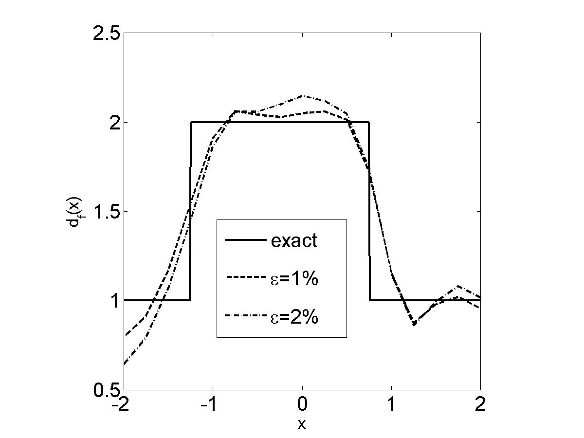
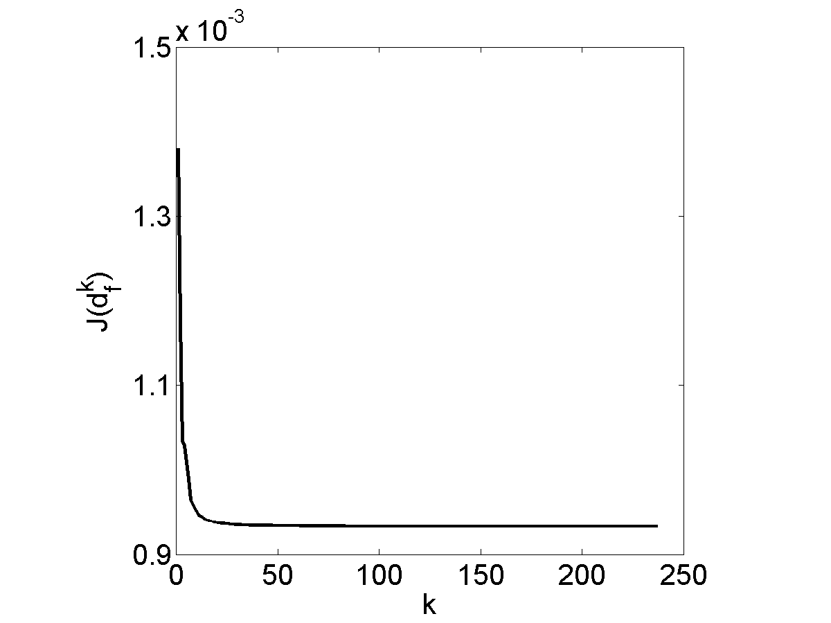
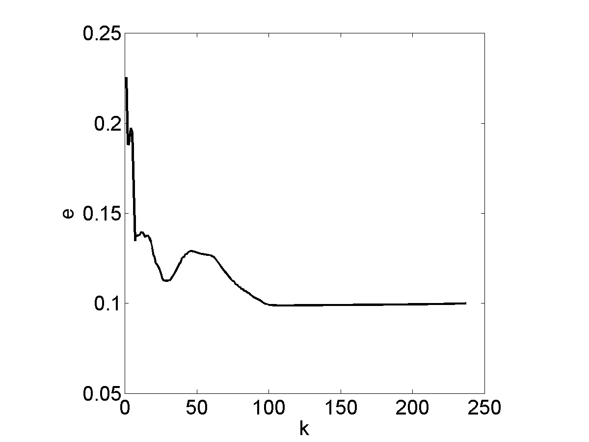
(a) reconstructions	(b) functional value $J(d_{f}^{k})$	(c) error $e$

Figure 2: Numerical results for Example 2. Here the convergence of Algorithm 1 is for $\varepsilon=2\%$ noise.

A last example considers the recovery of a more complex coefficient profile.

Example 3.

The boundary condition and initial condition of the problem are identical with those in Example 1. The exact coefficient $d_{f}^{\dagger}(x)$ is given by $d_{f}^{\dagger}=1-\frac{1}{2}\chi_{[-\frac{7}{8},-\frac{3}{8}]}+\frac{1}{2}\chi_{[\frac{5}{8},\frac{9}{8}]}$.

Here the true solution has more refined details, and hence the spatial mesh size $h$ is accordingly refined to $\frac{1}{8}$ for a better resolution. The results for Example 3 are shown in Figure 3 and Table 1. The convergence of the numerical reconstruction with respect to the noise level is again observed, see Table 1. The observations for the previous example remain valid: the numerical reconstructions roughly capture the profile of the true solution, but fail to resolve accurately the discontinuities, and the algorithm converges steadily and reasonably quick.

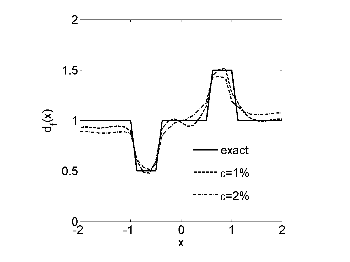
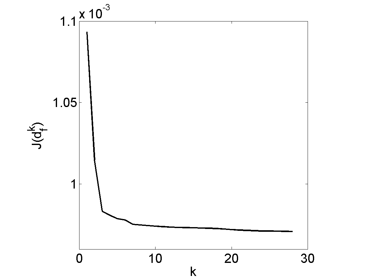
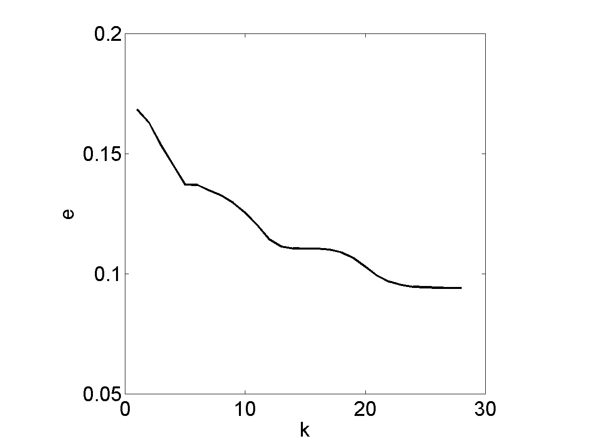
(a) reconstructions	(b) functional value $J(d_{f}^{k})$	(c) error $e$

Figure 3: Numerical results for Example 3. Here the convergence of Algorithm 1 is for $\varepsilon=2\%$ noise.

5 Concluding remarks

We have presented an inversion technique for estimating the Manning’s coefficient in the diffusive wave approximation of the shallow water equations. The results show that the proposed approach is capable of yielding an accurate and stable estimate in the presence of noise. We have also detailed a careful study of the properties of the forward map, in particular, we discuss its continuity and differentiability based on maximal regularity theory for parabolic problems. The mathematical analysis, such as, convergence and convergence rates, of such an inversion technique remains to be investigated. Also the evaluation of the method on real data is of significant interest.

Appendix A Properties of the forward map

In this part, we briefly discuss the continuity and differentiability of the forward map $F:L^{\infty}\rightarrow L^{2}(0,T;H^{1}(\Omega)),\ d_{f}\mapsto u(d_{f})$ based on maximal regularity theory for parabolic problems [10]. The conditions in Theorem A.1 impose a certain regularity constraint on the coefficient $d_{f}$ as well as on the boundary and initial conditions. Such mapping properties are essential for analyzing commonly used regularization schemes, for example, Tikhonov regularization and Landweber iteration for solving the inverse problem, and for establishing the convergence of numerical algorithms.

We first show the Lipschitz continuity of the forward map $F$.

Theorem A.1.

Assume that $\|u(d_{f})\|_{L^{\infty}}$ and $\|\nabla u(d_{f})\|_{L^{\infty}}$ are uniformly bounded, and that $d_{f}$, $|\nabla u(d_{f})|$ and $(u(d_{f})-z)$ are strictly positive, and further the gradient $|\nabla(t\,u(d_{f})+(1-t)u(\tilde{d}_{f}))|$ is strictly positive for all $t\in(0,1)$ and $d_{f},\tilde{d}_{f}$ in the admissible set $\mathcal{A}$. Then if $\gamma$ is sufficiently close to unity, the mapping $F:L^{\infty}\to L^{2}(0,T;H^{1}(\Omega))$ given by $d_{f}\mapsto u(d_{f})$ is Lipschitz continuous on $\mathcal{A}$.

Proof.

We denote by $k\left(u,\nabla u;d_{f}\right)=d_{f}\frac{(u-z)^{\alpha}}{|\nabla u|^{1-\gamma}}$ and $\tilde{u}=u(\tilde{d}_{f})$, and let $v=u-\tilde{u}$. We denote the bilinear form parametrized by $d_{f}$ as

$$B(u,w;d_{f})=(u_{t},w)+\left(k(u,\nabla u;d_{f})\nabla u,\nabla w\right),$$

By subtracting the bilinear forms $B(u,w;d_{f})=\ell(w)$ and $B(\tilde{u},w,\tilde{d_{f}})=\ell(w)$ and choosing $w=v$, we arrive at

$$0=\left(u_{t}-\tilde{u}_{t},w\right)+\left(k(u,\nabla u;d_{f})\nabla u-k(\tilde{u},\nabla\tilde{u};\tilde{d_{f}})\nabla\tilde{u},\nabla w\right),$$

which by virtue of the assumptions on $u$ and $\nabla u$ can be rearranged into

$$\dfrac{1}{2}\partial_{t}\|v\|^{2}_{L^{2}}+C_{K}\|\nabla v\|^{2}_{L^{2}}\leq -\left(k(u,\nabla u;{d_{f}-\tilde{d_{f}}})\nabla u,\nabla v\right)$$

$$-\left(\left(k(u,\nabla u;{\tilde{d_{f}}})-k(\tilde{u},\nabla\tilde{u};{\tilde{d_{f}}})\right)\nabla\tilde{u},\nabla v\right):=I+II,$$

where $C_{K}$ is the coercivity constant for the bilinear form $B(\cdot,\cdot)$. Using Cauchy-Schwarz inequality and Young’s inequality, the first summand $I$ on the right hand side can be estimated as follows

$$I\leq C(\epsilon_{1})\|d_{f}-\tilde{d_{f}}\|^{2}_{L^{\infty}}+\epsilon_{1}\|\nabla v\|^{2}_{L^{2}}.$$

Meanwhile, we split the nonlinear term in the bracket in the second summand $II$ into

$$k(u,\nabla u;\tilde{d_{f}})-k(\tilde{u},\nabla\tilde{u};\tilde{d_{f}})=d_{f}\left[\frac{\left(u-z\right)^{\alpha}\left(|\nabla{\tilde{u}}|^{1-\gamma}-|\nabla{u}|^{1-\gamma}\right)}{|\nabla{u}|^{1-\gamma}|\nabla{\tilde{u}}|^{1-\gamma}}+\frac{\left(u-z\right)^{\alpha}-\left(\tilde{u}-z\right)^{\alpha}}{|\nabla{\tilde{u}}|^{1-\gamma}}\right].$$ (2)

Now the mean value theorem gives

$$\left(u-z\right)^{\alpha}-\left(\tilde{u}-z\right)^{\alpha}=\alpha\left(\bar{u}-z\right)^{\alpha-1}v,$$ (3)

where $\bar{u}$ is an element between $u$ and $\tilde{u}$, and also by means of the Taylor expansion

$$|\nabla{\tilde{u}}|^{1-\gamma}-|\nabla{u}|^{1-\gamma}=\left(1-\gamma\right)\mathbf{v}\cdot\nabla v,$$ (4)

and the function

$$\mathbf{v}=\int_{0}^{1}\frac{\nabla(u-sv)}{|\nabla(u-sv)|^{1+\gamma}}ds,$$

which by assumption is bounded in $L^{\infty}$. Consequently by Young’s inequality, we get

$$II\leq \left(1-\gamma\right)\|k(u,\nabla u,\tilde{d_{f}})\|_{L^{\infty}}\|\mathbf{v}\|_{L^{\infty}}\|\nabla{\tilde{u}}\|^{\gamma}_{L^{\infty}}\|\nabla v\|^{2}_{L^{2}}+C\left(\epsilon_{2}^{-1}\|v\|^{2}_{L^{2}}+\tfrac{\epsilon_{2}}{4}\|\nabla v\|^{2}_{L^{2}}\right)$$

$$\leq C\left(\left(1-\gamma\right)+\epsilon_{2}\right)\|\nabla v\|^{2}_{L^{2}}+C\epsilon_{2}^{-1}\|v\|^{2}_{L^{2}}.$$

Since $\gamma$ is close to unity and for sufficiently small $\epsilon_{1}$, $\epsilon_{2}$, $\mu:=C\left(\left(1-\gamma\right)+\epsilon_{1}+\epsilon_{2}\right)<C_{K}$, we obtain

$$\tfrac{1}{2}\partial_{t}\|v\|^{2}_{L^{2}}+\left(C_{K}-\mu\right)\|\nabla v\|^{2}_{L^{2}}\leq C\epsilon_{2}^{-1}\|v\|^{2}_{L^{2}}+C\|d_{f}-\tilde{d_{f}}\|^{2}_{L^{\infty}}$$

Now an application of Gröwnwall’s inequality leads to

$$\|v\|^{2}_{L^{2}}+\int_{0}^{T}\|\nabla v\|^{2}_{L^{2}}ds\leq C\|d_{f}-\tilde{d_{f}}\|^{2}_{L^{\infty}}$$

upon noting the condition $u(0)=\tilde{u}(0)$. ∎

Our next result improves the regularity of the map in Theorem A.1 by invoking Gröger’s maximal regularity theory [10], which is needed for the differentiability.

Theorem A.2.

Let the assumptions in Theorem A.1 be fulfilled. Then the mapping $F:L^{\infty}\to L^{2}(0,T;W^{1,p}(\Omega))$, $d_{f}\mapsto u(d_{f})$ is Lipschitz continuous for some $p\in(2,\infty)$.

Proof.

As before, we denote by

$$k(u,\nabla u;d_{f})=d_{f}\frac{\left(u-z\right)^{\alpha}}{|\nabla u|^{1-\gamma}}$$

and $\tilde{u}=u(\tilde{d}_{f})$, and let $v=u-\tilde{u}$. Then $v$ solves

$$v_{t}+Av=f$$

with

$$Av=-\nabla\cdot\left(\left(k(u,\nabla u;\tilde{d_{f}})-k(\tilde{u},\nabla\tilde{u};\tilde{d_{f}})\right)\nabla\tilde{u}+k(u,\nabla u;\tilde{d}_{f})\nabla v\right)$$

and $f=\nabla\cdot\left(k(u,\nabla u;d_{f}-\tilde{d_{f}})\nabla u\right)$. Clearly, $f\in L^{p}(0,T;(W^{1,p})^{\prime})$ for $d_{f}-\tilde{d_{f}}\in L^{p}$ because the remaining terms are uniformly bounded in $L^{\infty}$. To apply Gröger’s theorem [10, Theorem 2.1], we only need to show the coercivity and boundedness of the operator $A$ defined above. By using the Taylor expansions (3) and (4) in the splitting (2), we can rearrange the differential $A$ into

$$\left(Av,w\right) =\left(k(u,\nabla u;\tilde{d}_{f})\left(1-\gamma\right)|\nabla\tilde{u}|^{\gamma-1}\mathbf{v}\cdot\nabla v\nabla\tilde{u},\nabla w\right)$$

$$-\left(\tilde{d_{f}}\alpha\left(\bar{u}-z\right)^{\alpha-1}|\nabla{\tilde{u}}|^{\gamma-1}v\nabla\tilde{u},\nabla w\right)+\left(k(u,\nabla u;\tilde{d}_{f})\nabla v,\nabla w\right).$$

In view of the strict positivity of the term $k(u,\nabla u;\tilde{d}_{f})$, that the parameter $\gamma$ is close to one and that the quantities $u,\,\nabla u$ etc. are uniformly bounded, we deduce that

$$\left(Av,v\right)\geq c_{A}\|\nabla v\|_{L^{2}}-C_{A}\|v\|_{L^{2}}.$$

for some constants $c_{A},\,C_{A}>0$. Hence, the associated matrix-valued coefficient in the differential operator is pointwise bounded from below and above away from zero. The continuity of the operator follows similarly. Consequently, an application of Gröger’s theorem [10] directly yields the desired estimate $\int_{0}^{T}\|v(s)\|_{W^{1,p}}^{2}ds\leq C\|d\|_{L^{\infty}}$ for some $p\in(2,\infty)$. ∎

Remark A.1.

The exponent $p\in(2,\infty)$ in Theorem A.2 depends on the spatial dimension, the pointwise upper and lower bounds of the conductivity $k(u,\nabla u;d_{f})$ and the smoothness of the domain $\Omega$; see [10] for details.

Next we show the boundedness of the linearized map.

Theorem A.3.

Let the assumptions in Theorem A.1 be fulfilled, and the linear map $F^{\prime}:L^{\infty}\to L^{2}(0,T;H^{1}(\Omega))$ be defined by $d\mapsto v$, with $v$ given by

$$\left(v_{t},w\right)+ \left(k(u,\nabla u)[I-\left(1-\gamma\right)\tilde{\eta}\otimes\tilde{\eta}]\cdot\nabla v,\nabla w\right)$$

$$+\left(d_{f}\alpha\frac{\left(u-z\right)^{\alpha-1}v}{|\nabla u|^{1-\gamma}}\nabla u,\nabla w\right)=-\left(d\frac{\left(u-z\right)^{\alpha}}{|\nabla u|^{1-\gamma}}\nabla u,\nabla w\right),$$

with the initial condition $v(0)=0$. Then the linear map $F^{\prime}$ is bounded.

Proof.

Insert $w:=v$ to get

$$\tfrac{1}{2}\partial_{t}\|v\|^{2}_{L^{2}(\Omega)}+ \left(k(u,\nabla u;d_{f})\nabla v,[I-\left(1-\gamma\right)\tilde{\eta}\otimes\tilde{\eta}]\nabla v\right)$$

$$=-\left(d_{f}\alpha\frac{\left(u-z\right)^{\alpha-1}v}{|\nabla u|^{1-\gamma}}\nabla u,\nabla v\right)-\left(d\frac{\left(u-z\right)^{\alpha}}{|\nabla u|^{1-\gamma}}\nabla u,\nabla v\right):=I+II.$$

Using Cauchy-Schwarz inequality and Young’s inequality, the term $I$ can be bounded by

$$I\leq C(\epsilon_{1})\|d_{f}\|^{2}_{L^{\infty}}\|\left(u-z\right)^{\alpha-1}|\nabla u|^{\gamma}\|^{2}_{L^{\infty}}\|v\|^{2}_{L^{2}}+\epsilon_{1}\|\nabla v\|^{2}_{L^{2}},$$

where $\epsilon_{1}>0$ is arbitrary. Similarly, the term $II$ can be bounded by: for any $\epsilon_{2}>0$

$$II\leq C(\epsilon_{2})\|d\|^{2}_{L^{\infty}}\|d_{f}\|^{2}_{L^{\infty}}\|\left(u-z\right)^{\alpha}|\nabla u|^{\gamma}\|^{2}_{L^{2}}+\epsilon_{2}\|\nabla v\|^{2}_{L^{2}}.$$

Recall that $\gamma$ is strictly less than unity, and hence $I-\left(1-\gamma\right)\tilde{\eta}\otimes\tilde{\eta}$ is strictly positive definite, and the diffusion coefficient $k(u,\nabla u;d_{f})$ is strictly positive (independent of $d_{f}$). Therefore, these estimates altogether give

$$\tfrac{1}{2}\partial_{t}\|v\|^{2}_{L^{2}(\Omega)}+\|\nabla v\|^{2}_{L^{2}}\leq C\left(\|v\|^{2}_{L^{2}}+\|d\|^{2}_{L^{\infty}}\right).$$

Applying Grönwall’s inequality and noting that $v(0)=0$, the desired assertion follows. ∎

Remark A.2.

The condition that the parameter $\gamma$ is close to $1$ is not required in Theorem A.3. A direct application of Gröger’s theorem indicates that the map $F^{\prime}:L^{\infty}\mapsto L^{p}(0,T;W^{1,p}(\Omega))$ is also bounded.

Finally, we show the Fréchet differentiability of the forward map.

Theorem A.4.

Let the assumptions in Theorem A.1 be fulfilled, and the bounded linear map $u^{\prime}(d_{f})d$ be defined in Theorem A.3. Then $u^{\prime}(d_{f})d$ is the Fréchet derivative of the map $d_{f}\rightarrow u(d_{f})$, i.e.,

$$\lim_{\|d\|_{L^{\infty}}\to 0}\frac{\|u(d_{f}+d)-u(d_{f})-u^{\prime}(d_{f})d\|_{L^{2}(0,T;H^{1}(\Omega))}}{\|d\|_{L^{\infty}}}=0.$$

Proof.

We denote by $k(u,\nabla u;d_{f})=d_{f}\frac{\left(u-z\right)^{\alpha}}{|\nabla u|^{1-\gamma}}$ and $\tilde{d}_{f}=d_{f}+d$, $\tilde{u}=u(\tilde{d}_{f})$, $u=u(d_{f})$ and $\bar{u}=u^{\prime}(d_{f})d$ and let $v=\tilde{u}-u$, $w=\tilde{u}-u-\bar{u}$. We also denote $D(u)=\left(1-\gamma\right)\tilde{\eta}\otimes\tilde{\eta}$. Then it directly follows from the weak formulations for $\tilde{u}$, $u$ and $\bar{u}$ that

$$\left(w_{t},w\right)+ \left(k(\tilde{u},\nabla\tilde{u};\tilde{d}_{f})\nabla\tilde{u}-k(u,\nabla u;\tilde{d}_{f})\nabla u,\nabla w\right)$$

$$= \left(k(u,\nabla u;d_{f})\left(I-D(u)\right)\nabla\bar{u},\nabla w\right)+\left(d_{f}\alpha\frac{\left(u-z\right)^{\alpha-1}\bar{u}}{|\nabla u|^{1-\gamma}}\nabla u,\nabla w\right),$$

which upon rearrangement and noting the assumptions on $u$ and $\nabla u$ yields

$$(w_{t},w)+(k(u,\nabla u;\tilde{d}_{f})\nabla w,\nabla w)= \underbrace{((k(u,\nabla u;\tilde{d}_{f})-k(\tilde{u},\nabla\tilde{u};\tilde{d}_{f}))\nabla\tilde{u},\nabla w)}_{I}\underbrace{-(k(u,\nabla u;d)\nabla\bar{u},\nabla w)}_{II}$$

$$-\underbrace{(k(u,\nabla u;d_{f})D(u)\nabla\bar{u},\nabla w)}_{III}+\underbrace{\left(d_{f}\alpha\frac{(u-z)^{\alpha-1}\bar{u}}{|\nabla u|^{1-\gamma}}\nabla u,\nabla w\right)}_{IV}.$$

It suffices to estimate the four terms on the right hand side. First, by means of Cauchy-Schwarz inequality and Young’s inequality, the term $II$ can be estimated by

$$|II|\leq C\|d\|_{L^{\infty}}\|\nabla\bar{u}\|_{L^{2}}\|\nabla w\|_{L^{2}},$$

To bound the first term $I$, we further split it into

$$I=\left(k(u,\nabla u;\tilde{d}_{f})\frac{(|\nabla{\tilde{u}}|^{1-\gamma}-|\nabla{u}|^{1-\gamma})}{|\nabla{\tilde{u}}|^{1-\gamma}}\nabla\tilde{u},\nabla w\right)+\left(\tilde{d}_{f}\frac{(u-z)^{\alpha}-(\tilde{u}-z)^{\alpha}}{|\nabla{\tilde{u}}|^{1-\gamma}}\nabla\tilde{u},\nabla w\right):=V+VI.$$

Now we employ the Taylor expansion

$$|\nabla\tilde{u}|^{1-\gamma}=|\nabla u|^{1-\gamma}+(1-\gamma)|\nabla u|^{-\gamma-1}\nabla u\cdot\nabla v+\boldsymbol{K}\nabla v^{2}$$

with the matrix-valued function $\boldsymbol{K}$ given by

$$\boldsymbol{K}=-\int_{0}^{1}(1-t)\left((1-\gamma^{2})\boldsymbol{\phi}(t)\boldsymbol{\phi}(t)^{\mathrm{t}}|\boldsymbol{\phi}(t)|^{-\gamma-3}+(1-\gamma)|\boldsymbol{\phi}(t)|^{-1-\gamma}\boldsymbol{I}\right)dt$$

and $\boldsymbol{\phi}(t)=\nabla(u+tv)$. With the help of this expansion, we derive that

$$V-III =(k(u,\nabla u;d_{f})D(u)\nabla w,\nabla w)+(1-\gamma)\underbrace{\left(k(u,\nabla u;d_{f})\frac{\nabla u\cdot\nabla v}{|\nabla u|}\left(\frac{|\nabla u|^{1-\gamma}\nabla\tilde{u}}{|\nabla\tilde{u}|^{1-\gamma}|\nabla u|}-\frac{\nabla u}{|\nabla u|}\right),\nabla w\right)}_{VII}$$

$$+(1-\gamma)\underbrace{\left(k(u,\nabla u;d)\frac{\nabla u\cdot\nabla v}{|\nabla u|^{1+\gamma}}\frac{\nabla\tilde{u}}{|\nabla\tilde{u}|^{1-\gamma}},\nabla w\right)}_{VIII}+\underbrace{\left(k(u,\nabla u;\tilde{d}_{f})\frac{\boldsymbol{K}\nabla v^{2}}{|\nabla\tilde{u}|^{1-\gamma}}\nabla\tilde{u},\nabla w\right)}_{IX}$$

Next we estimate the terms on the right-hand side one by one. First, let $p$ be the exponent from theorem A.2 and choose $q>2$ such that $\frac{1}{p}+\frac{1}{q}=\frac{1}{2}$. Then by the uniform $L^{\infty}$ boundness of $u$ and $\nabla u$ (also $\tilde{u}$, $\nabla\tilde{u}$ etc.)

$$VII =\left(k(u,\nabla u;d_{f})\frac{\nabla u\cdot\nabla v}{|\nabla u|^{2}}|\nabla\tilde{u}|^{\gamma-1}\left(|\nabla u|^{1-\gamma}\nabla v+\nabla u(|\nabla u|^{1-\gamma}-|\nabla\tilde{u}|^{1-\gamma})\right),\nabla w\right)$$

$$\leq C\|\nabla v\|_{L^{p}}\|\nabla v\|_{L^{q}}\|\nabla w\|_{L^{2}}+C\||\nabla v|(|\nabla u|^{1-\gamma}-|\nabla\tilde{u}|^{1-\gamma})\|_{L^{2}}\|\nabla w\|_{L^{2}}$$

$$\leq C\|\nabla v\|_{L^{p}}\|\nabla v\|_{L^{q}}\|\nabla w\|_{L^{2}}+C\||\nabla v|^{2}\|_{L^{2}}\|\nabla w\|_{L^{2}}$$

$$\leq C\|\nabla v\|_{L^{p}}\|\nabla v\|_{L^{q}}\|\nabla w\|_{L^{2}}\leq C\|\nabla v\|^{1+\delta}_{L^{p}}\|\nabla w\|_{L^{2}},$$

where in the third line we have utilized the expansion (4), and the last line follows from the fact that either $\|\nabla v\|_{L^{q}}\leq C\|\nabla v\|_{L^{p}}$ holds for $q<p$ or $\|\nabla v\|_{L^{q}}\leq C\|\nabla v\|^{\delta}_{L^{p}}$ holds for some $0<\delta<1$ due to the $L^{\infty}$-boundedness of $\nabla u$ and $\nabla\tilde{u}$. Similarly, the terms $VIII$ and $IX$ can be bounded by

$$VIII\leq C\|d\|_{L^{\infty}}\|\nabla v\|_{L^{2}}\|\nabla w\|_{L^{2}}\quad\mbox{and}\quad IX\leq C\|\nabla v\|^{1+\delta}_{L^{p}}\|\nabla w\|_{L^{2}}.$$

Next we combine the terms $VI$ and $IV$. To this end, we employ the Taylor expansion

$$(\tilde{u}-z)^{\alpha}=(u-z)^{\alpha}+\alpha(u-z)^{\alpha-1}v+\tfrac{1}{2}\alpha(\alpha-1)(\hat{u}-z)^{\alpha-2}v^{2}$$

with $\hat{u}$ being some function pointwise between $u$ and $\tilde{u}$ we can estimate. With the help of this identity, we arrive at the following splitting

$$VI+IV =-\left(d_{f}\alpha\frac{(u-z)^{\alpha-1}w}{|\nabla u|^{1-\gamma}}\nabla u,\nabla w\right)+\underbrace{\left(d_{f}\alpha(u-z)^{\alpha-1}v\left(\frac{\nabla u}{|\nabla u|^{1-\gamma}}-\frac{\nabla\tilde{u}}{|\nabla{\tilde{u}}|^{1-\gamma}}\right),\nabla w\right)}_{X}$$

$$-\underbrace{\left(d\alpha\frac{(u-z)^{\alpha-1}}{|\nabla{\tilde{u}}|^{1-\gamma}}v\nabla\tilde{u},\nabla w\right)}_{XI}-\underbrace{\tfrac{1}{2}\left(\tilde{d}_{f}\alpha(\alpha-1)\frac{(\eta-z)^{\alpha-2}}{|\nabla{\tilde{u}}|^{1-\gamma}}v^{2}\nabla\tilde{u},\nabla w\right)}_{XII}$$

Consequently, by the uniform boundedness of the quantities $u$, $\nabla u$ (and $\tilde{u}$, $\nabla\tilde{u}$ etc.) and Sobolev embedding theorem, we have

$$X\leq C\|v\|_{W^{1,P}}^{1+\delta}\|\nabla w\|_{L^{2}},\quad XI\leq C\|d\|_{L^{\infty}}\|v\|_{W^{1,p}}\|\nabla w\|_{L^{2}},\quad XII\leq C\|\nabla v\|^{1+\delta}_{W^{1,p}}\|\nabla w\|_{L^{2}}.$$

These estimates, Young’s inequality and that $\gamma$ is close to unity (hence $D(u)$ can be made arbitrarily small for $\gamma$ close to unity) yield

$$\tfrac{1}{2}\partial_{t}\|w\|^{2}_{L^{2}}+\tfrac{C_{K}}{2}\|\nabla w\|^{2}_{L^{2}}\leq C\left(\|d\|_{L^{\infty}}^{2}\|v\|_{W^{1,p}}^{2}+\|v\|_{W^{1,p}}^{2+2\delta}+\|w\|_{L^{2}}^{2}\right).$$

Finally, an application of Grönwall’s inequality and Theorem A.2 lead to

$$\|w\|^{2}_{L^{2}}+\int_{0}^{T}\|\nabla w\|^{2}_{L^{2}}ds\leq C\|d\|^{2+2\delta}_{L^{\infty}}$$

upon noting the initial condition $w(0)=0$. This concludes the proof. ∎

Remark A.3.

An inspection of the proof indicates that the assumptions on the solution $u(d_{f})$ and gradient can be greatly relaxed if the parameter $\gamma=1$. The latter case is analogous to the porous media equation, and thus the results are of independent interest.

Appendix B Generalized-$\alpha$ method

In this appendix, we describe the generalized-$\alpha$ method. Note that for the full discretization of the forward problem, each time step involves solving a highly nonlinear (and possibly also stiff) system. Hence a careful treatment of the time stepping is required. To this end, we employ the so-called generalized-$\alpha$ method together with a predictor-corrector method [14, 5]. For a first-order system, the method can be stated as follows: given $(u_{n},\dot{u}_{n})$, find $(u_{n+1},\dot{u}_{n+1},u_{n+\alpha_{f}},\dot{u}_{n+\alpha_{m}})$ such that

$$\left\{\begin{aligned} R(u_{n+\alpha_{f}},\dot{u}_{n+\alpha_{m}})&=0,\\ u_{n+\alpha_{f}}&=u_{n}+\alpha_{f}(u_{n+1}-u_{n}),\\ \dot{u}_{n+\alpha_{m}}&=\dot{u}_{n}+\alpha_{m}(\dot{u}_{n+1}-\dot{u}_{n}),\\ u_{n+1}&=u_{n}+\Delta t((1-\gamma)\dot{u}_{n}+\gamma\dot{u}_{n+1}),\end{aligned}\right.$$

where $\Delta t=t_{n+1}-t_{n}$ is the time step size, $\alpha_{f}$, $\alpha_{m}$ and $\gamma$ are real valued parameters of the method, and $R(u_{n+\alpha_{f}},\dot{u}_{n+\alpha_{m}})$ denotes the (discrete) residual of the nonlinear system. For a linear model problem, unconditional stability of the scheme is attained if $\alpha_{m}\geq\alpha_{f}\geq\frac{1}{2}$, and a second-order accuracy can be achieved with the choice $\gamma=\frac{1}{2}+\alpha_{m}-\alpha_{f}$ [14]. The method can be succinctly parameterized by the spectral radius $\rho_{\infty}$ into a one-parameter family. Then the parameters $\alpha_{m}$, $\alpha_{f}$ and $\gamma$ can be expressed as [14]

$$\alpha_{f}=\frac{1}{1+\rho_{\infty}},\quad\alpha_{m}=\frac{3-\rho_{\infty}}{2(1+\rho_{\infty})},\quad\gamma=\frac{1}{1+\rho_{\infty}}.$$

A complete description of the generalized-$\alpha$ method is given in Algorithm 2. It is of predictor/corrector type with correctors computed by a Newton method, where the superscript indices indicate the corrector steps within the loop. In our implementation, we have set $\rho_{\infty}=0.1$, and the tolerance $\epsilon$ in the stopping criterion to $1.0\times 10^{-6}$ and the maximum number of iterations ($\mathrm{MaxIter}$) to $20$. The major computational effort of Algorithm 2 lies in calculating the Jacobian matrix $K_{n+1}^{(i)}$ for the Newton system, i.e., step $5$. For large-scale problems, iterative solvers, e.g., GMRES or BiCGstab, which requires only matrix-vector multiplication, are preferable [14].

Algorithm 2 Generalized-$\alpha$ method.

1:  Compute predictor $u_{n+1}^{(0)}=u_{n}$ and $\dot{u}_{n+1}^{(0)}=\frac{\gamma-1}{\gamma}\dot{u}_{n}$, and set $i=0$.

2:  Set the initial guess of $u_{n+\alpha_{f}}^{(0)}$ and $u_{n+\alpha_{m}}^{(0)}$ as

$$u_{n+\alpha_{f}}^{(0)}=u_{n}+\alpha_{f}(u_{n+1}^{(0)}-u_{n})\quad\mbox{and}\quad\dot{u}_{n+\alpha_{m}}^{(0)}=\dot{u}_{n}+\alpha_{m}(\dot{u}_{n+1}^{(0)}-\dot{u}_{n}).$$

3:  while $i<\mathrm{MaxIter}$ do

4:     Evaluate the Newton residual $\displaystyle R_{n+1}^{(i)}=R(u_{n+\alpha_{f}}^{(i)},\dot{u}_{n+\alpha_{m}}^{(i)})$.

5:     Calculate the Jacobian

$$K_{n+1}^{(i)}=\frac{\partial R(u_{n+\alpha_{f}}^{(i)},\dot{u}_{n+\alpha_{m}}^{(i)})}{\partial u_{n+\alpha_{f}}}+\alpha_{m}[\alpha_{f}\gamma\Delta t]^{-1}\frac{\partial R(u_{n+\alpha_{f}}^{(i)},\dot{u}_{n+\alpha_{m}}^{(i)})}{\partial\dot{u}_{n+\alpha_{m}}}.$$

6:     Solve Newton system for the corrector $\Delta u_{n+1}^{(i)}$ from $K_{n+1}^{(i)}\Delta u_{n+1}^{(i)}=-R_{n+1}^{(i)}$.

7:     Update the solutions $u_{n+\alpha_{f}}^{(i+1)}$ and $\dot{u}_{n+\alpha_{m}}^{(i+1)}$ by

$$u_{n+\alpha_{f}}^{(i+1)} =u_{n+1}^{(i)}+\Delta u_{n+1}^{(i)},$$

$$\dot{u}_{n+\alpha_{m}}^{(i+1)} =(1-\gamma^{-1}\alpha_{m})\dot{u}_{n+1}^{(i)}+\alpha_{m}[\gamma\Delta t\alpha_{f}]^{-1}(u_{n+\alpha_{f}}^{(i+1)}-u_{n}).$$

8:     Check the stopping criterion: if $\displaystyle\|R_{n+1}^{(i)}\|\leq\epsilon\|R_{n+1}^{(0)}\|$, stop iteration.

9:     Increase index $i=i+1$.

10:  end while

11:  Output the solutions $u_{n+1}$ and $\dot{u}_{n+1}$ by

$$u_{n+1}=u_{n}+\alpha_{f}^{-1}(u_{n+\alpha_{f}}^{(\mathrm{MaxIter})}-u_{n})\quad\mbox{and}\quad\dot{u}_{n+1}=\dot{u}_{n}+\alpha_{m}^{-1}(\dot{u}_{n+\alpha_{m}}^{(\mathrm{MaxIter})}-\dot{u}_{n}).$$

References

- [1] O. M. Alifanov. Inverse Heat Transfer Problems. Springer-Verlag, Berlin, 1994.
- [2] R. Alonso, M. Santillana, and C. Dawson. On the diffusive wave approximation of the shallow water equations. Eur. J. Appl. Math., 19(5):575–606, 2008.
- [3] G. J. Arcement and V. R. Schneider. Guide for Selecting Manning’s Roughness Coefficient for Natural Channels and Flood Plains. Water-Supply Paper No. 2339 (Department of the Interior, U.S. Geological Survey, Reston, VA, 1990).
- [4] V. T. Chow. Open-Channel Hydraulics. McGraw-Hill, New York, 1988.
- [5] N. Collier, H. Radwan, L. Dalcin, and V. M. Calo. Diffusive wave approximation to the shallow water equations: computational approach. Proc. Comput. Sci., 4:1828–1833, 2011.
- [6] Y. Ding, Y. Jia, and S. S. Y. Wang. Identification of manning’s roughness coefficients in shallow water flows. J. Hydr. Eng., 130(6):501–510, 2004.
- [7] Y. Ding and S. S. Y. Wang. Identification of manning’s roughness coefficients in channel network using adjoint analysis. Int. J. Comput. Fluid Dyn., 19(1):3–13, 2005.
- [8] K. Feng and F. J. Molz. A 2-d diffusion based, wetland flow model. J. Hydrol., 196(1–4):230–250, 1997.
- [9] P. Gauckler. Etudes théoriques et pratiques sur l’ecoulement et le mouvement des eaux. Comptes Rendues de l’Académie des Sciences, Paris, France, 64:818–822, 1867.
- [10] K. Gröger. -estimates of solutions to evolution equations corresponding to nonsmooth second order elliptic differential operators. Nonlinear Anal., 18(6):569–577, 1992.
- [11] W. W. Hager and H. Zhang. A survey of the nonlinear conjugate gradient methods. Pac. J. Optimiz., 2:35–58, 2006.
- [12] T. V. Hromadka II, C. E. Berenbrock, J. R. Freckleton, and G. L. Guymon. A two-dimensionaldam-break flood plain model. Adv. Water Res., 8(1):7– 14, 1985.
- [13] K. Ito, B. Jin, and T. Takeuchi. A regularization parameter for nonsmooth Tikhonov regularization. SIAM J. Sci. Comput., 33(3):1415–1438, 2011.
- [14] K. E. Jansen, C. H. Whiting, and G. M. Hulbert. A generalized- method for integrating the filtered navier-stokes equations with a stabilized finite element method. Comput. Methods Appl. Mech. Engrg., 190:305–319, 2000.
- [15] B. Jin, Y. Zhao, and J. Zou. Iterative parameter choice by discrepancy principle. IMA J. Numer. Anal., page in press, 2012.
- [16] B. Jin and J. Zou. Numerical estimation of the Robin coefficient in a stationary diffusion equation. IMA J. Numer. Anal., 30(3):677–701, 2010.
- [17] M. Santillana and C. Dawson. A numerical approach to study the properties of the solutions of the diffusive wave approximation of the shallow water equations. Comput. Geosci., 14(1):31–53, 2010.
- [18] A. N. Tikhonov and V. Y. Arsenin. Solutions of Ill-Posed Problems. John Wiley & Sons, New York, 1977.
- [19] D. Walkowiak, editor. Open Channel Flow Measurement Handbook. Teledyne ISCO, 6th edition, 2006.
- [20] T. Xanthopoulos and C. Koutitas. Numerical simulation of a two-dimensional flood wave propagation due to dam failure. J. Hydr. Res., 14(4):321–331, 1976.
- [21] B. C. Yen, editor. Channel Flow Resistance: Centennial of Manning’s Formula. Water Resources Publications, Highlands Branch, Colorado, 1992.