Abstract

Spatial solitary waves in colloidal suspensions of spherical dielectric nanoparticles are considered. The interaction of the nanoparticles is modelled as a hard-sphere gas, with the Carnahan-Starling formula used for the gas compressibility. Semi-analytical solutions, for both one and two spatial dimensions, are derived using an averaged Lagrangian and suitable trial functions for the solitary waves. Power versus propagation constant curves and neutral stability curves are obtained for both cases, which illustrate that multiple solution branches occur for both the one and two dimensional geometries. For the one-dimensional case it is found that three solution branches (with a bistable regime) occur, while for the two-dimensional case two solution branches (with a single stable branch) occur in the limit of low background packing fractions. For high background packing fractions the power versus propagation constant curves are monotonic and the solitary waves stable for all parameter values. Comparisons are made between the semi-analytical and numerical solutions, with excellent comparison obtained.

Keywords. colloid, solitary wave, modulation theory, stability, bifurcation.
AMS (MOS) subject classification: 35, 78.

1 Introduction

Over the last two decades the mechanical interaction between light and soft matter has received considerable attention, including the emergence of new tools in optics, such as optical tweezers and traps, see [8, 12, 3]. In the colloidal medium considered here, which is composed of a suspension of dielectric nanoparticles, the exceptionally high optical nonlinearity is due to the optical gradient force changing the concentration or orientation of the colloidal particles. This leads to an intensity-dependent refractive index change and hence a mutual interaction between the colloidal particles and light. Possible new applications in colloidal media include optical sensors or selective particle trapping and manipulation. Spatial solitary waves form in a colloidal medium due to a balance between diffraction of the light beam and the nonlinear particle-light interaction.

[17, 18, 19] derived colloidal media governing equations by assuming that the colloidal suspension represents a hard-sphere gas. They used the Carnahan-Starling formula for the compressibility of the hard-sphere colloid. They then considered one and two dimensional colloidal equations and derived numerically exact propagation constant versus power curves. They showed that bistable behaviour occurs for some parameter values and considered solitary wave interactions for solitary waves of the same power, from the same and different solution branches. They found dramatically different interaction behaviour for solitons from the same and different branches. In the 2-D case, only two solution branches can occur and the bistable behaviour of the 1-D colloidal solitary wave is absent.

[20] considered a colloidal suspension of two different species of nanoparticles, one with refractive index higher than the background medium and the other with refractive index lower than the background medium. One species is described by a hard-sphere gas with the Carnahan-Starling compressibility formula and the other by an ideal gas. Numerical solitary wave solutions were found for the governing equations which show that bistability can occur for the two-dimensional geometry, which is not possible for suspensions composed of only a single nanoparticle species.

[9] modelled a colloidal suspension of nanoparticles as an ideal gas and considered two cases, one for which the refractive index of the nanoparticles was greater than the background medium, and the other for which the refractive index is lower. The governing equation in the two cases of positive and negative polarizability was an NLS-type equation with exponential nonlinearity and a form of saturable exponential nonlinearity, respectively. The stability of the solitary waves solutions was considered numerically in one and two spatial dimensions. [10] considered a power series for the compressibility of the colloid particles with the coefficients of the series found by using the Debye-Huckel model for the particle interactions. This interaction model included screening effects due to the ions in the electrolyte solution. Solitary wave stability was considered, with one-dimensional waves found to be stable and two-dimensional waves unstable. [16] experimentally considered the nonlinear optical response of a nanoparticle suspension and found that a higher-order NLS equation with coefficients fitted from a two term series expansion for the compressibility best matched the experimental data.

The governing equation for wave propagation in colloidal media is an NLS-type equation for which the form of the nonlinearity in the NLS-type equation depends on the assumed nature of the nanoparticle interactions. No exact solitary wave solutions exist for these NLS-type equations, so most existing work on has been numerical or based on a mix of various asymptotic, approximate and numerical methods. An effective technique for deriving semi-analytical solutions describing the stability and evolution of solitary waves in NLS-type systems is a variational approach. This approach is termed modulation theory and is based on using an averaged Lagrangian and suitable trial functions. It has been used to study the NLS equation [14] and optical media, such as nematic liquid crystals [21]. Related applications and problems considered for nematic media include dipole motion, boundary induced motion and the development of bores [11, 2, 4].

In §1 modulation theory is developed for the colloidal equations studied here. A hard-sphere colloidal model is used with the compressibility described by the Carnahan-Starling formula. Semi-analytical solutions for both one and two-dimensional solitary waves are developed. In §2 the modulation equations are solved numerically to obtain semi-analytical power versus propagation constant curves and neutral stability curves. These curves illustrate the multiplicity of the solitary wave solution branches and the regions of parameter space in which unstable solutions occur. An excellent comparison between the semi-analytical and numerical solutions is obtained. In §3 conclusions and suggestions for future work are made.

2 Modulation equations

Let us consider a coherent light beam (laser light) propagating through a colloidal suspension of dielectric hard spheres whose diameter is much smaller than the wavelength of the light and whose refractive index is slightly higher than that of the medium in which they are suspended. With these assumptions, in non-dimensional form the equations governing the nonlinear propagation of the beam through the colloidal suspension are (see [17, 18])

$$i\frac{\partial u}{\partial z}+\frac{1}{2}\nabla^{2}u+\left(\eta-\eta_{0}\right)u=0,\ \ |u|^{2}=g(\eta)-g_{0},$$ (1)

$${\rm with}\ \ g(\eta)=\frac{3-\eta}{(1-\eta)^{3}}+\ln\eta,\ \ g_{0}=g(\eta_{0}).$$

Here $u$ is the envelope of the electric field of the light and $\eta$ is the packing fraction of the colloid particles, with $\eta_{0}$ the background fraction. Losses due to Rayleigh scattering have been neglected as these losses are small in the limit of the particle diameter being much smaller than the wavelength of the light [18]. The Carnahan-Starling compressibility approximation has been used. Alternative models for the compressibility alter the form of $g$ in (1). The Carnahan-Starling approximation is valid up to the solid-fluid transition, which occurs at $\eta=\sqrt{2}\pi/9\approx 0.496$ in a hard-sphere fluid, see [13].

The colloid equations (1) have the Lagrangian formulation

$$L=i\left(u^{*}u_{z}-uu^{*}_{z}\right)-|\nabla u|^{2}+2\left(\eta-\eta_{0}\right)|u|^{2}-\frac{4-2\eta}{(1-\eta)^{2}}$$ (2)

$$\mbox{}+\frac{4-2\eta_{0}}{(1-\eta_{0})^{2}}-2\eta\ln\eta+2\eta_{0}\ln\eta_{0}+2\left(\eta-\eta_{0}\right)(1+g_{0}).$$

Here the asterisk superscript denotes the complex conjugate. The colloid equations (1) possess solitary wave solutions. However the solitary wave solutions, in both 1-D and 2-d, have only been found numerically [18, 19], with no analytical solution known. An approximate technique which has been found to be useful in these cases for which there is no known analytical solution on which to base a perturbation analysis is the use of suitable trial functions in an averaged Lagrangian formulation [14]. In the special case in which there is an analytical solitary wave, or periodic wave, solution this approximate technique is the same as the modulation theory or averaged Lagrangian technique of Whitham [23] and other, related, perturbation techniques [14]. In this sense this use of trial functions in an averaged Lagrangian is an extension of Whitham modulation theory. The approximate trial function method has been applied to many problems in nonlinear optics and has been found to give solutions in excellent agreement with numerical and experimental results [21, 6]. The key is to find a good approximation to the solitary wave solution of a given equation. However, in many situations, the evolution of the beam, in particular its position and velocity, are independent, or nearly so, of the form of the trial function used for the solitary wave profile [22, 5, 7]. This use of trial functions in an averaged Lagrangian, termed modulation theory in analogy with the modulation theory of Whitham [23], will be used to analyse solitary wave solutions of the present colloid equations.

2.1 One spatial dimension

Let us first consider the solitary wave solution of the 1-D form of the colloid equations (1). The solitary wave solution of the nonlinear Schrödinger (NLS) equation in 1-D has a $\mathop{\rm sech}\nolimits$ profile. In the small colloid concentration limit $\eta\ll 1$ the colloid equations (1) reduce to the NLS equation. Therefore, let us use the trial functions

$$u=a\mathop{\rm sech}\nolimits\frac{x-\xi}{w}\>e^{i\sigma+iV(x-\xi)}+ige^{i\sigma+iV(x-\xi)},\quad\eta=\eta_{0}+\alpha\mathop{\rm sech}\nolimits^{2}\frac{x-\xi}{\beta}$$ (3)

for the electric field and colloid fraction to analyse the evolution of an initial beam to a steady solitary wave solution. The parameters are all functions of $z$. They are the amplitudes, $a$ and $\alpha$, and the widths, $w$ and $\beta$, of the electric field and colloid fraction, respectively. $\sigma$ is the propagation constant of the solitary wave, while $\xi^{\prime}=V$ is the velocity of the solitary wave. Lastly, $g$ is the amplitude of the radiation bed on which the beam sits. The first term in the electric field solitary wave is a varying NLS-type solitary wave. The second term represents the low wavenumber (long wavelength) radiation that accumulates under an evolving beam which is not an exact solitary wave solution. The origin of this low wavenumber radiation is explained in detail in [14]. However, its origin can be deduced from the group velocity $c_{g}=k$ for linear waves of wavenumber $k$ for the NLS-type equation (1). It can be seen that low wavenumber waves have low group velocity and so accumulate under the beam as it evolves. This flat shelf of radiation under the beam matches to shed radiation of non-zero wavenumber which propagates away from the beam and so allows it to settle to a steady state [14]. The flat shelf of radiation cannot extend indefinitely and so is assumed to have length $\ell$, so that $g$ is non-zero in $\xi-\ell/2\leq x\leq\xi+\ell/2$ [14]. Finally the flat shelf under the beam is $\pi/2$ out of phase with it, which accounts for the $i$ multiplying $g$ in the trial function for $u$ [14]. As previously mentioned, the flat shelf links with the shed diffractive radiation which propagates away from the beam. The effect of this shed radiation could be included [14]. However, for the present analysis the effect of this shed radiation is not needed.

Substituting the trial functions (3) into the Lagrangian (2) and averaging it by integrating in $x$ over the infinite domain results in the averaged Lagrangian

$${\cal L}=-2\left(2a^{2}w+\ell g^{2}\right)(\sigma^{\prime}-V\xi^{\prime}+V^{2}/2)-2\pi awg^{\prime}+2\pi gwa^{\prime}$$ (4)

$$+2\pi gaw^{\prime}-\frac{2}{3}\frac{a^{2}}{w}+4\alpha a^{2}\Omega_{1}(w,\beta)-\beta\Xi_{1}(\alpha)-4\beta\Theta_{1}(\alpha)$$

$$+4\alpha\beta\left(1+g_{0}\right),\ \ {\rm where}$$

$$\Omega_{1}(w,\beta)=\int_{0}^{\infty}\mathop{\rm sech}\nolimits^{2}\frac{\zeta}{\beta}\mathop{\rm sech}\nolimits^{2}\frac{\zeta}{w}\>d\zeta,$$

$$\Xi_{1}(\alpha)=2\int_{0}^{\infty}\left[\frac{4-2\eta_{0}-2\alpha\mathop{\rm sech}\nolimits^{2}\zeta}{(1-\eta_{0}-\alpha\mathop{\rm sech}\nolimits^{2}\zeta)^{2}}-\frac{4-2\eta_{0}}{(1-\eta_{0})^{2}}\right]\>d\zeta,$$

$$\Theta_{1}(\alpha)=\int_{0}^{\infty}\left[\eta_{0}\ln(1+\frac{\alpha}{\eta_{0}}\mathop{\rm sech}\nolimits^{2}\zeta)+\alpha\mathop{\rm sech}\nolimits^{2}\zeta\ln\left(\eta_{0}+\alpha\mathop{\rm sech}\nolimits^{2}\zeta\right)\right]\>d\zeta.$$

Taking variations of this averaged Lagrangian with respect to the solitary wave parameters gives the modulation equations

$$\frac{d}{dz}\left(2a^{2}w+\ell g^{2}\right)=0,$$ (5)

$$\pi\frac{d}{dz}aw=\ell g(\sigma^{\prime}-V\xi^{\prime}+V^{2}/2),$$ (6)

$$\pi\frac{dg}{dz}=\frac{2a}{3w^{2}}-\frac{2\alpha a}{w}(\Omega_{1}-w\Omega_{1w}),$$ (7)

$$\frac{d\sigma}{dz}-V\frac{d\xi}{dz}+\frac{1}{2}V^{2}=-\frac{1}{2w^{2}}+\frac{\alpha}{w}(2\Omega_{1}-w\Omega_{1w}),$$ (8)

$$\frac{d}{dz}\left(2a^{2}w+\ell g^{2}\right)V=0,\ \ \frac{d\xi}{dz}=V,$$ (9)

$$4a^{2}\Omega_{1}-\beta\Xi_{1\alpha}-4\beta\Theta_{1\alpha}+4\beta\left(1+g_{0}\right)=0,$$ (10)

$$4\alpha a^{2}\Omega_{1\beta}-\Xi_{1}-4\Theta_{1}+4\alpha\left(1+g_{0}\right)=0.$$ (11)

Equation (5) is conservation of mass, while the first of equations (9) is conservation of momentum, in the sense of invariances of the Lagrangian (2), see [15]. However, in the present optical context (5) corresponds physically to conservation of optical power.

A steady solitary wave solution of (1) will not shed radiation, so that $g=0$ at the fixed point of the modulation equations. Also, at the steady state we can set $V=\xi=0$ for convenience. Note that a simple transformation generates non-stationary solitary waves (with $V$ non-zero) with an unchanged profile. Setting $g=V=\xi=0$ in the modulation equations gives

$$1-3\alpha w(\Omega_{1}-w\Omega_{1w})=0,$$ (12)

$$\sigma^{\prime}+\frac{1}{2w^{2}}-\frac{\alpha}{w}(2\Omega_{1}-w\Omega_{1w})=0,$$ (13)

$$4a^{2}\alpha(\Omega_{1}-\beta\Omega_{1\beta})-\beta(\alpha\Xi_{1\alpha}-\Xi_{1})-4\beta(\alpha\Theta_{1\alpha}-\Theta_{1})=0,$$ (14)

$$4\alpha a^{2}\Omega_{1\beta}-\Xi_{1}-4\Theta_{1}+4\alpha\left(1+g_{0}\right)=0.$$ (15)

These four transcendental equations in the five unknowns $a$, $\alpha$, $w$, $\beta$ and $\sigma^{\prime}$ represent a two-parameter family of solitary waves which depend on $\eta_{0}$. The optical power is defined by

$$P=\int_{-\infty}^{\infty}|u(x)|^{2}\>dx.$$ (16)

Using the trial function (3) in (16) gives the power of the 1-D semi-analytical solitary wave as

$$P=\int_{-\infty}^{\infty}a^{2}\mathop{\rm sech}\nolimits^{2}{x\over w}\>dx=2a^{2}w.$$ (17)

Semi-analytical power versus propagation constant curves are described by the solution of (12)–(15). Stable solution branches occur for $P_{\sigma}>0$ (see [18]). Hence solitary waves of neutral stability have the property that $P_{\sigma}=0$. Adding this condition to the equations (12)–(15) gives a set of five equations for the five unknowns, for given $\eta_{0}$. Hence, the curves of neutral stability are lines in the $\sigma$ versus $\eta_{0}$ plane. The relevant sets of transcendental equations for both the power versus propagation constant curves and the lines of neutral stability were solved using a nonlinear equation solver from the IMSL library.

2.2 Two spatial dimensions

The modulation equations of the previous subsection for the evolution of a beam in a 1-D can be extended to a 2-D beam. In this case the appropriate trial functions are

$$u=a\mathop{\rm sech}\nolimits\frac{\phi}{w}\>e^{i\sigma+iU(x-\xi_{x})+iV(y-\xi_{y})}+ige^{i\sigma+iU(x-\xi_{x})+iV(y-\xi_{y})},$$ (18)

$$\eta=\eta_{0}+\alpha\mathop{\rm sech}\nolimits^{2}\frac{\phi}{\beta},\ \ {\rm where}\ \ \phi=\sqrt{(x-\xi_{x})^{2}+(y-\xi_{y})^{2}}.$$

Substitution of these trial functions into the Lagrangian (2) and integrating in $x$ and $y$ from $-\infty$ to $\infty$ results in the averaged Lagrangian

$${\cal L}=-2\left(I_{2}a^{2}w^{2}+\Lambda g^{2}\right)(\sigma^{\prime}-U\xi_{x}^{\prime}-V\xi_{y}^{\prime}+U^{2}/2+V^{2}/2)$$ (19)

$$-2I_{1}aw^{2}g^{\prime}+2I_{1}gw^{2}a^{\prime}+4I_{1}awgw^{\prime}-I_{22}a^{2}+2\alpha a^{2}\Omega_{2}(w,\beta)$$

$$-\beta^{2}\Xi_{2}(\alpha)-2\beta^{2}\Theta_{2}(\alpha)+2I_{2}\alpha\beta^{2}\left(1+g_{0}\right).$$

In this 2-D case the shelf of low wavenumber radiation under the beam forms a circle of radius $\ell$, so that $g$ is non-zero in the circle

$$0\leq\sqrt{(x-\xi_{x})^{2}+(y-\xi_{y})^{2}}\leq\ell.$$ (20)

Here $\Lambda=\ell^{2}/2$. The various integrals involved in this averaged Lagrangian are

$$I_{1}=\int_{0}^{\infty}\zeta\mathop{\rm sech}\nolimits\zeta\>d\zeta=2C,\ \ I_{2}=\int_{0}^{\infty}\zeta\mathop{\rm sech}\nolimits^{2}\zeta\>d\zeta=\ln 2,$$

$$I_{22}=\int_{0}^{\infty}\zeta\mathop{\rm sech}\nolimits^{2}\zeta\tanh^{2}\zeta\>d\zeta=\frac{1}{3}\ln 2+\frac{1}{6},$$

$$\Omega_{2}(w,\beta)=\int_{0}^{\infty}\zeta\mathop{\rm sech}\nolimits^{2}\frac{\zeta}{\beta}\mathop{\rm sech}\nolimits^{2}\frac{\zeta}{w}\>d\zeta,$$ (21)

$$\Xi_{2}(\alpha)=\int_{0}^{\infty}\zeta\left[\frac{4-2\eta_{0}-2\alpha\mathop{\rm sech}\nolimits^{2}\zeta}{(1-\eta_{0}-\alpha\mathop{\rm sech}\nolimits^{2}\zeta)^{2}}-\frac{4-2\eta_{0}}{(1-\eta_{0})^{2}}\right]\>d\zeta,$$

$$\Theta_{2}(\alpha)=\int_{0}^{\infty}\zeta\left[\eta_{0}\ln(1+\frac{\alpha}{\eta_{0}}\mathop{\rm sech}\nolimits^{2}\zeta)\right.$$

$$\left.\mbox{}+\alpha\mathop{\rm sech}\nolimits^{2}\zeta\ln\left(\eta_{0}+\alpha\mathop{\rm sech}\nolimits^{2}\zeta\right)\right]\>d\zeta,$$

where $C$ is the Catalan constant $C=0.915965594\ldots$ [1]. The modulation (variational) equations for the averaged Lagrangian (19) are

$$\frac{d}{dz}\left(I_{2}a^{2}w^{2}+\Lambda g^{2}\right)=0,$$ (22)

$$I_{1}\frac{d}{dz}aw^{2}=\Lambda g(\sigma^{\prime}-U\xi_{x}^{\prime}-V\xi_{y}^{\prime}+U^{2}/2+V^{2}/2),$$ (23)

$$2I_{1}\frac{dg}{dz}=\frac{I_{22}a}{w^{2}}-\frac{\alpha a}{w^{2}}\left(2\Omega_{2}-w\Omega_{2w}\right),$$ (24)

$$I_{2}\left(\frac{d\sigma}{dz}-U\frac{d\xi_{x}}{dz}-V\frac{d\xi_{y}}{dz}+\frac{1}{2}U^{2}+\frac{1}{2}V^{2}\right)=$$

$$\mbox{}-\frac{I_{22}}{w^{2}}+\frac{\alpha}{2w^{2}}(4\Omega_{2}-w\Omega_{2w}),$$ (25)

$$\frac{d}{dz}\left(I_{2}a^{2}w^{2}+\Lambda g^{2}\right)U=0,\ \ \frac{d}{dz}\left(I_{2}a^{2}w^{2}+\Lambda g^{2}\right)V=0,$$ (26)

$$\frac{d\xi_{x}}{dz}=U,\ \ \frac{d\xi_{y}}{dz}=V,$$ (27)

$$2a^{2}\Omega_{2}-\beta^{2}\Xi_{2\alpha}-2\beta^{2}\Theta_{2\alpha}+2I_{2}\beta^{2}\left(1+g_{0}\right)=0,$$ (28)

$$\alpha a^{2}\Omega_{2\beta}-\beta\Xi_{2}-2\beta\Theta_{2}+2I_{2}\alpha\beta\left(1+g_{0}\right)=0.$$ (29)

At the steady-state we have $g=V=U=\xi=0$ and the modulation equations become

$$I_{22}-\alpha\left(2\Omega_{2}-w\Omega_{2w}\right)=0,$$ (30)

$$I_{2}\sigma^{\prime}+\frac{I_{22}}{w^{2}}-\frac{\alpha}{2w^{2}}(4\Omega_{2}-w\Omega_{2w})=0,$$ (31)

$$2a^{2}\Omega_{2}-\beta^{2}\Xi_{2\alpha}-2\beta^{2}\Theta_{2\alpha}+2I_{2}\beta^{2}\left(1+g_{0}\right)=0,$$ (32)

$$\alpha a^{2}\Omega_{2\beta}-\beta\Xi_{2}-2\beta\Theta_{2}+2I_{2}\alpha\beta\left(1+g_{0}\right)=0.$$ (33)

As in the 1-D case, equations (30)–(33) give a semi-analytical description of a two parameter family of 2-D colloidal solitary waves. The optical power of these solitary waves is given by

$$P=\int_{0}^{\infty}r|u(r)|^{2}\>dr.$$ (34)

The power of a semi-analytical 2-D solitary wave is then found by substituting the trial function (18) into (34), giving

$$P=\int_{0}^{\infty}ra^{2}\mathop{\rm sech}\nolimits^{2}{r\over w}\>dr=a^{2}w^{2}\ln 2.$$ (35)

3 Results and discussion

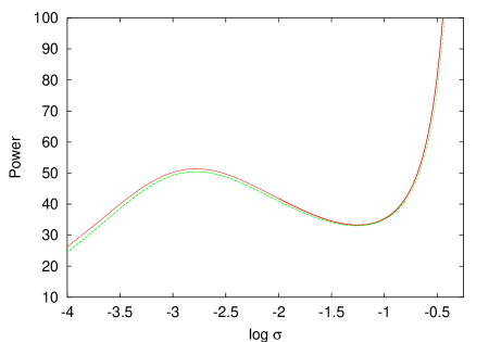
Figure 1: The power versus propagation constant ($P$ versus log $\sigma$) curve for the 1-D colloidal solitary wave. Shown are the semi-analytical (solid lines, red) and numerical (dashed lines, green) solutions. The background fraction is $\eta_{0}=1\times 10^{-3}$.

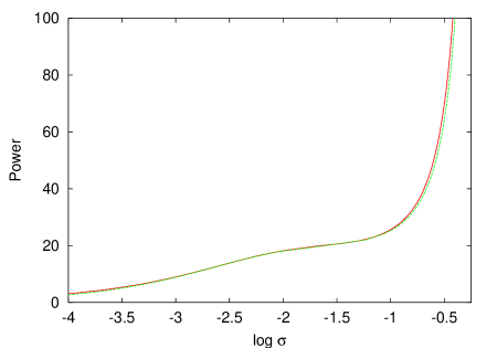
Figure 2: The power versus propagation constant ($P$ versus log $\sigma$) curve for the 1-D colloidal solitary wave. Shown are the semi-analytical (solid lines, red) and numerical (dashed lines, green) solutions. The background fraction is $\eta_{0}=1\times 10^{-2}$.

In this section the semi-analytical solutions for colloidal solitary waves are compared with numerical solutions. Semi-analytical estimates for the power versus propagation constant and neutral stability curves are both found. The numerical solutions in 1-D are obtained by analytically integrating the steady-state version of the governing equation to obtain an energy conservation law. The energy conservation law can then be numerically integrated to obtain exact solitary wave profiles on both the stable and unstable solution branches or the power versus propagation constant curves. In 2-D the numerical solutions were obtained using the imaginary time iterative method suitable for obtaining numerically exact solitary wave profiles [24]. Note that the imaginary time method cannot be used to obtain numerical solutions on an unstable solution branch.

3.1 One spatial dimension

Figure 1 shows the power versus propagation constant ($P$ versus ${\rm log}\sigma$) curve for the 1-D colloidal solitary wave. The background packing fraction is $\eta_{0}=1\times 10^{-3}$. Shown are the semi-analytical solution (12)–(15) and the numerical solution. The figure uses the same parameters as Figure 3 of [18]. It can be seen that there is an excellent comparison between the semi-analytical and numerical solutions. The figure shows two stable branches, separated by a middle, unstable solution branch. The solitary waves on the low power stable branch have low amplitudes and large widths, whilst those on the high power stable branch have large amplitudes and smaller widths. The semi-analytical solution indicates that the middle unstable branch exists for

$$-2.77<{\rm log}\sigma<-1.25\ \ {\rm and}\ \ 33.26<P<51.37$$ (36)

$$1.31<a<2.29\ \ {\rm and}\ \ 4.29\times 10^{-3}<\alpha<0.19.$$

Figure 2 shows the power versus propagation constant ($P$ versus $\log\sigma$) curve for the 1-D colloidal solitary wave for the background packing fraction $\eta_{0}=1\times 10^{-2}$. Shown are the semi-analytical solution (12)–(15) and the numerical solution. In this example the background packing fraction has been increased, which eliminates the bistability. The propagation constant versus power curve now has a single, stable solution branch. Again the comparison between the semi-analytical and numerical solutions is excellent. Figures 1 and 2 illustrate that the semi-analytical solution is extremely accurate and hence is highly suitable for obtaining accurate results relating to the stability and other properties of 1-D colloidal solitary waves.

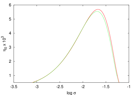
Figure 3: The neutral stability curve in the propagation constant-background packing fraction plane ($\log\sigma$,$\eta_{0}$) for the 1-D colloidal solitary wave. Shown are the semi-analytical (solid lines, red) and numerical (dashed lines, green) solutions.

Figure 3 shows the neutral stability curve in the propagation constant-background packing fraction plane ($\log\sigma$, $\eta_{0}$) for the 1-D colloidal solitary wave. Shown are the semi-analytical and numerical solutions. The semi-analytical and numerical neutral stability curves were found by solving the condition $P_{\sigma}=0$ using the expressions for both the semi-analytical and numerical power. The region under the curves represents parameter values corresponding to the middle, unstable branch of solitary wave solutions. The figure shows that as the background packing fraction increases, the region of parameter space in which unstable solutions occur is reduced and then eliminated. The parameters of the solitary wave with neutral stability at the turning point are

$$({\rm log}\sigma,\eta_{0},a,\alpha)=(-1.67,5.69\times 10^{-3},1.71,5.65\times 10^{-2}),$$ (37)

$$({\rm log}\sigma,\eta_{0},a,\alpha)=(-1.69,5.54\times 10^{-3},1.72,5.79\times 10^{-2}),$$ (38)

where (37) and (38) are the semi-analytical and numerical solitary waves, respectively. It can be seen that the semi-analytical prediction of the background packing fraction at the turning point is extremely accurate, with less than $3\%$ error. Hence bistable behaviour only occurs in 1-D geometry for $\eta_{0}\leq 5.54\times 10^{-3}$ and a single stable solution branch exists for background packing fractions greater than this value. This is consistent with the bistable curve of Figure 1 and the monotone stability seen in Figure 2.

3.2 Two spatial dimensions

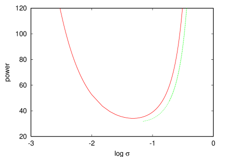
Figure 4: The power versus propagation constant ($P$ versus $\log\sigma$) curve for the 2-D colloidal solitary wave. Shown are the semi-analytical (solid lines, red) and numerical (dashed lines, green) solutions. The background fraction is $\eta_{0}=1\times 10^{-3}$.

Figure 4 shows the power versus propagation constant ($P$ versus $\log\sigma$) curve for the 2-D colloidal solitary wave. The background packing fraction is $\eta_{0}=1\times 10^{-3}$. Shown are the semi-analytical solution (12)–(15) and the numerical solution. This figure is qualitatively different from the 1-D case of Figure 1 as the bistable behaviour is absent. There are two solution branches, one stable and the other unstable. The stable solution branch corresponds to solitary waves of large amplitude. The semi-analytical theory predicts that the stable branch occurs for

$$\sigma>0.06,\ \ a>3.81\ \ {\rm and}\ \ \alpha>0.46.$$ (39)

The comparison between the semi-analytical and numerical solutions is very good; there is a $17\%$ difference in the power and a $6\%$ difference in the amplitude $a$ at $\sigma=0.18$. Note that the maximum packing fraction of the stable solitary wave of minimum amplitude is $\eta=\alpha+\eta_{0}=0.461$, which is close to the value $\eta\approx 0.496$ at which solidification occurs in the hard sphere model. Hence this branch of stable solitary waves is unlikely to be realised in real colloidal suspensions.

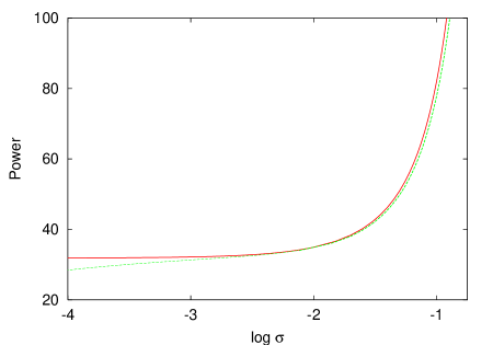
Figure 5: The power versus propagation constant ($P$ versus log $\sigma$) curve for the 2-D colloidal solitary wave. Shown are the semi-analytical (solid lines, red) and numerical (dashed lines, green) solutions. The background fraction is $\eta_{0}=0.3$.

Figure 5 shows the power versus propagation constant ($P$ versus $\log\sigma$) curve for the 2-D colloidal solitary wave for the background packing fraction $\eta_{0}=0.3$. Shown are the semi-analytical solution (30)–(33) and the numerical solution. For this much larger value of the background packing fraction there is only one stable solution branch. Hence, multiple solution branches occur in both the 1-D and 2-D cases only if the background packing fraction is small enough. The comparison between the semi-analytical and numerical solutions is again excellent, except for some slight variation for $\log\sigma<-3$. For larger powers the amplitudes of the electric field and colloidal fraction pulses increase; beyond $P\approx 50$ the hard-sphere colloid model predicts solidification. As in the 1-D case the comparison between the semi-analytical and numerical solutions is excellent and confirms the suitability of semi-analytical methods for understanding colloidal wave stability.

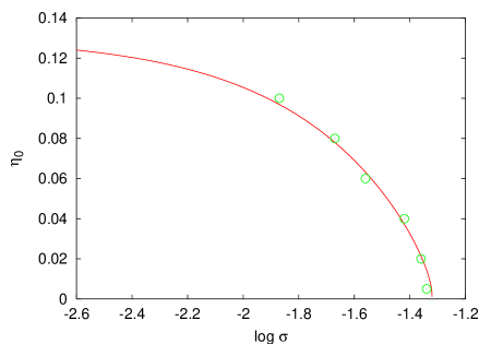
Figure 6: The neutral stability curve in the propagation constant-background packing fraction plane ($\log\sigma$, $\eta_{0}$) for the 2-D colloidal solitary wave. Shown is the semi-analytical solution (solid line, red) and numerical solutions (circles, green).

Figure 6 shows the neutral stability curve in the propagation constant-background packing fraction plane ($\log\sigma$, $\eta_{0}$) for the 2-D colloidal solitary wave. Shown are the semi-analytical and numerical solutions. The semi-analytical solution is found by solving (30)–(33) and the condition $P_{\sigma}=0$. The numerical solutions are found using the imaginary time iterative method, which is used to find stable solitary wave solutions. For a given background packing fraction, the numerically obtained solution of minimum power is shown. This solution lies close to the turning point on the propagation constant versus power curve, and is a numerical estimate of the neutrally stable solitary wave. The region to the left of the semi-analytical curve represents parameter values corresponding to the unstable branch of solitary wave solutions. The curve indicates that multiple solitary wave solution branches only occur for $\eta_{0}<0.125$ and that for larger background packing fractions a single stable solution branch occurs. As the semi-analytical curve of neutral stability is traversed from right to left the amplitude of the colloid beam decreases. It can be seen that there is an excellent comparison between the semi-analytical curve and numerical estimates for the neutrally stable solitary wave. No numerical estimates near $\eta_{0}=0.125$ are presented due to computational difficulties in resolving marginally unstable and stable cases. This is related to the fact that, in this limit, the propagation constant versus power curve becomes very nearly flat.

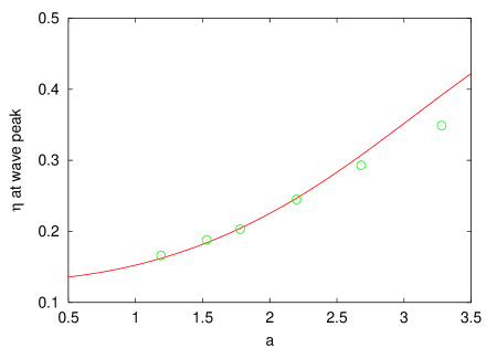
Figure 7: The neutral stability curve in the amplitude-maximum packing fraction plane ($a$, $\eta$) for the 2-D colloidal solitary wave. Shown is the semi-analytical solution (solid line, red) and numerical solutions (circles, green).

Figure 7 shows the neutral stability curve in the amplitude-maximum packing fraction plane ($a$, $\eta$) for the 2-D colloidal solitary wave. Shown are the semi-analytical and numerical solutions. The semi-analytical solution is found by solving (30)–(33) and the condition $P_{\sigma}=0$. The numerical solutions are found using the imaginary time iterative method, which is used to find stable solitary wave solutions. The region below the semi-analytical curve represents parameter values corresponding to the unstable branch of solitary wave solutions. This alternative view of the neutral stability curve shows the peak electric field intensity and colloid packing fraction of the neutrally stable solitary waves. As the curve is traversed from left to right the background packing fraction decreases from $\eta_{0}=0.125$ to zero. Hence stable solitary waves have large maximum packing fractions when $\eta_{0}$ is small. As solidification occurs for $\eta\geq 0.496$, it can be seen that physically realistic, but stable, solitary waves occur for a small range of amplitudes in the small background packing fraction limit. As for figure 6, the comparison between semi-analytical and numerical solutions is excellent.

4 Conclusions

In this paper a semi-analytical model for colloidal solitary waves described by the hard-sphere gas model with the Carnahan-Starling approximation has been developed. Power versus propagation constant curves have been derived for both 1-D and 2-D geometries, with an excellent comparison with numerical solutions obtained. The neutral stability curves show that multiple solution branches only occur for low background packing fractions. The critical background packing fractions at which multiplicity is lost are well determined by the semi-analytical theory.

Future work using the semi-analytical model will involve a number of directions. Firstly, the semi-analytical theory will be used to examine the unsteady evolution of colloidal beams and the development of colloidal undular bores. This approach has been been shown to be successful in tackling these problems in related optical media, such as nematic liquid crystals [4]. Secondly, the semi-analytical tools developed here can be used to analyse other possible colloidal models which use different gas compressibility laws or are composed of multiple nanoparticle species with different optical properties [20]. This will help our understanding of the stability regimes for 2-D beams in experimental scenarios involving physically important colloidal materials.

5 Acknowledgements

This research was supported by the Royal Society of London under grant JP090179.

Received August 2010; revised February 2011; revised September 2011.
http://monotone.uwaterloo.ca/$\sim$journal/

References

- [1] M. Abramowitz and I.A. Stegun, Handbook of Mathematical Functions with Formulas, Graphs and Mathematical Tables, Dover Publications, Inc., New York (1972).
- [2] A. Alberucci, G. Assanto, D. Buccoliero, A. Desyatnikov, T.R. Marchant and N.F. Smyth, “Modulation analysis of boundary induced motion of nematicons,” Phys. Rev. A, 79, 043816 (2009).
- [3] A. Ashkin, J.M. Dziedzic, J.E. Bjorkholm and S. Chu, “Observation of a single-beam gradient force optical trap for dielectric particle,” Opt. Lett., 11, 288 (1986).
- [4] G. Assanto, T.R. Marchant and N.F. Smyth, “Collisionless shock resolution in nematic liquid crystals,” Phys. Rev. A, 78, 063808 (2008).
- [5] G. Assanto, B.D. Skuse and N.F. Smyth, “Optical path control of spatial optical solitary waves in dye-doped nematic liquid crystals,” Photon. Lett. Poland, 1, 154–156 (2009).
- [6] G. Assanto, A.A. Minzoni, M. Peccianti and N.F. Smyth, “Optical solitary waves escaping a wide trapping potential in nematic liquid crystals: modulation theory,” Phys. Rev. A, 79, 033837 (2009).
- [7] G. Assanto, B.D. Skuse and N.F. Smyth, “Solitary wave propagation and steering through light-induced refractive potentials,” Phys. Rev. A, 81, 063811 (2010).
- [8] M. Daoud and C.E. Williams eds., Soft Matter Physics, Springer (1999).
- [9] R. El-Ganainy, D.N. Christodoulies, C. Rotschild and M. Segev, “Soliton dynamics and self-induced transparency in nonlinear suspensions,” Opt. Express, 15, 10207–10218 (2007).
- [10] R. El-Ganainy, D.N. Christodoulies, E.M. Wright, W.M. Lee and K. Dholakia, “Nonlinear optical dynamics in nonideal gases of interacting colloidal nanoparticles,” Phy. Rev. A, 80, 053805 (2009).
- [11] C. García-Reimbert, A.A. Minzoni, T.R. Marchant, N.F. Smyth and A.L. Worthy, “Dipole soliton formation in a nematic liquid crystal in the nonlocal limit,” Physica D, 237, 1088–1102 (2008).
- [12] D.V. Grier, “A revolution in optical manipulation,” Nature, 424, 810 (2003).
- [13] J.P. Hansen and I.R. McDonald, Theory of Simple Liquids, Academic Press, London (1976).
- [14] W.L. Kath and N.F. Smyth, “Soliton evolution and radiation loss for the nonlinear Schrödinger equation,” Phys. Rev. E, 51, 1484–1492 (1995).
- [15] D.J. Kaup and A.C. Newell, “Solitons as particles, oscillators, and in slowly changing media: a singular perturbation theory,” Proc. Roy. Soc. Lond. A, 361, 413–446 (1978).
- [16] W.M. Lee, R. El-Ganainy, D.N. Christodoulies, K. Dholakia and E.M. Wright, “Nonlinear optical response of colloidal suspensions,” Opt. Express, 17, 10277–10289 (2009).
- [17] M. Matuszewski, W. Krolikowski and Y.S. Kivshar, “Spatial solitons and light-induced instabilities in colloidal media,” Opt. Express, 16, 1371–1376 (2008).
- [18] M. Matuszewski, W. Krolikowski and Y.S. Kivshar, “Soliton interactions and transformations in colloidal media,” Phys. Rev. A, 79, 023814 (2009).
- [19] M. Matuszewski, W. Krolikowski and Y.S. Kivshar, “Bistable solitons in colloidal media,” Photon. Lett. Poland, 1, 4–6 (2009).
- [20] M. Matuszewski, “Engineering optical soliton bistability in colloidal media,” Phy. Rev. A, 81, 013820, (2010).
- [21] A.A. Minzoni, N.F. Smyth and A.L. Worthy, “Modulation solutions for nematicon propagation in non-local liquid crystals,” J. Opt. Soc. Amer. B, 24, 1549–1556 (2007).
- [22] B.D. Skuse and N.F. Smyth, “Two-colour vector soliton interactions in nematic liquid crystals in the local response regime,” Phys. Rev. A, 77, 013817 (2008).
- [23] G.B. Whitham, Linear and Nonlinear Waves, J. Wiley and Sons, New York (1974).
- [24] J. Yang and T.I. Lakoba, “Accelerated imaginary-time evolution methods for the computation of solitary waves”, Stud. Appl. Math., 120, 265-292 (2008).