The asymptotics of ranking algorithms

Abstract

We consider the predictive problem of supervised ranking, where the task is to rank sets of candidate items returned in response to queries. Although there exist statistical procedures that come with guarantees of consistency in this setting, these procedures require that individuals provide a complete ranking of all items, which is rarely feasible in practice. Instead, individuals routinely provide partial preference information, such as pairwise comparisons of items, and more practical approaches to ranking have aimed at modeling this partial preference data directly. As we show, however, such an approach raises serious theoretical challenges. Indeed, we demonstrate that many commonly used surrogate losses for pairwise comparison data do not yield consistency; surprisingly, we show inconsistency even in low-noise settings. With these negative results as motivation, we present a new approach to supervised ranking based on aggregation of partial preferences, and we develop $U$-statistic-based empirical risk minimization procedures. We present an asymptotic analysis of these new procedures, showing that they yield consistency results that parallel those available for classification. We complement our theoretical results with an experiment studying the new procedures in a large-scale web-ranking task.

, and

t1Supported by DARPA through the National Defense Science and Engineering Graduate Fellowship Program (NDSEG). t2Supported in part by the U.S. Army Research Laboratory and the U.S. Army Research Office under contract/Grant W911NF-11-1-0391.

1 Introduction

Recent years have seen significant developments in the theory of classification, most notably binary classification, where strong theoretical results are available that quantify rates of convergence and shed light on qualitative aspects of the problem Zhang04b , BartlettJoMc06 . Extensions to multi-class classification have also been explored, and connections to the theory of regression are increasingly well understood, so that overall a satisfactory theory of supervised machine learning has begun to emerge Zhang04a , Steinwart07 .

In many real-world problems in which labels or responses are available, however, the problem is not merely to classify or predict a real-valued response, but rather to list a set of items in order. The theory of supervised learning cannot be considered complete until it also provides a treatment of such ranking problems. For example, in information retrieval, the goal is to rank a set of documents in order of relevance to a user’s search query; in medicine, the object is often to rank drugs in order of probable curative outcomes for a given disease; and in recommendation or advertising systems, the aim is to present a set of products in order of a customer’s willingness to purchase or consume. In each example, the intention is to order a set of items in accordance with the preferences of an individual or population. While such problems are often converted to classification problems for simplicity (e.g., a document is classified as “relevant” or not), decision makers frequently require the ranks (e.g., a search engine must display documents in a particular order on the page). Despite its ubiquity, our statistical understanding of ranking falls short of our understanding of classification and regression. Our aim here is to characterize the statistical behavior of computationally tractable inference procedures for ranking under natural data-generating mechanisms.

We consider a general decision-theoretic formulation of the supervised ranking problem in which preference data are drawn i.i.d. from an unknown distribution, where each datum consists of a query, $Q\in\mathcal{Q}$, and a preference judgment, $Y\in\mathcal{Y}$, over a set $m$ of candidate items that are available based on the query $Q$. The exact nature of the query and preference judgment depend on the ranking context. In the setting of information retrieval, for example, each datum corresponds to a user issuing a natural language query and expressing a preference by selecting or clicking on zero or more of the returned results. The statistical task is to discover a function that provides a query-specific ordering of items that best respects the observed preferences. This query-indexed setting is especially natural for tasks like information retrieval in which a different ranking of webpages is needed for each natural language query.

Following existing literature, we estimate a scoring function $f\dvtx\mathcal{Q}\rightarrow\mathbb{R}^{{m}}$, where $f(q)$ assigns a score to each of ${m}$ candidate items for the query $q$, and the results are ranked according to their scores HerbrichGrOb00 , FreundIyScSi03 . Throughout the paper, we adopt a decision-theoretic perspective and assume that given a query-judgment pair $(Q,Y)$, we evaluate the scoring function $f$ via a loss $L(f(Q),Y)$. The goal is to choose the $f$ minimizing the risk

$$R(f):=\mathbb{E}\bigl{[}L\bigl{(}f(Q),Y\bigr{)}\bigr{]}.$$ (1)

While minimizing the risk (1) directly is in general intractable, researchers in machine learning and information retrieval have developed surrogate loss functions that yield procedures for selecting $f$. Unfortunately, as we show, extant procedures fail to solve the ranking problem under reasonable data generating mechanisms. The goal in the remainder of the paper is to explain this failure and to propose a novel solution strategy based on preference aggregation.

Let us begin to elucidate the shortcomings of current approaches to ranking. One main problem lies in their unrealistic assumptions about available data. The losses proposed and most commonly used for evaluation in the information retrieval literature ManningRaSc08 , JarvelinKe04 have a common form, generally referred to as (Normalized) Discounted Cumulative Gain ((N)DCG). The NDCG family requires that the preference judgments $Y$ associated with the datum $(Q,Y)$ be a vector $Y\in\mathbb{R}^{m}$ of relevance scores for the entire set of items; that is, $Y_{j}$ denotes the real-valued relevance of item $j$ to the query $Q$. While having complete preference information makes it possible to design procedures that asymptotically minimize NDCG losses (e.g., CossockZh08 ), in practice such complete preferences are unrealistic: they are expensive to collect and difficult to trust. In biological applications, evaluating the effects of all drugs involved in a study—or all doses—on a single subject is infeasible. In web search, users click on only one or two results: no feedback is available for most items. Even when practical and ethical considerations do not preclude collecting complete preference information from participants in a study, a long line of psychological work highlights the inconsistency with which humans assign numerical values to multiple objects (e.g., ShiffrinNo94 , StewartBrCh05 , Miller56 ).

The inherent practical difficulties that arise in using losses based on relevance scores has led other researchers to propose loss functions that are suitable for partial preference data Joachims02 , FreundIyScSi03 , DekelMaSi03 . Such data arise naturally in a number of real-world situations; for example, a patient’s prognosis may improve or deteriorate after administration of treatment, competitions and sporting matches provide paired results, and shoppers at a store purchase one item but not others. Moreover, the psychological literature shows that human beings are quite good at performing pairwise distinctions and forming relative judgments (see, e.g., Saaty08 and references therein).

More formally, let $\alpha:=f(Q)\in\mathbb{R}^{m}$ denote the vector of predicted scores for each item associated with query $Q$. If a preference $Y$ indicates that item $i$ is preferred to $j$ then the natural associated loss is the zero-one loss $L(\alpha,Y)=1({\alpha_{i}\leq\alpha_{j}})$. Minimizing such a loss is well known to be computationally intractable; nonetheless, the classification literature Zhang04a , Zhang04b , BartlettJoMc06 , Steinwart07 has shown that it is possible to design convex Fisher-consistent surrogate losses for the 0–1 loss in classification settings and has linked Fisher consistency to consistency. By reduction to classification, similar consistency results are possible in certain bipartite or binary ranking scenarios ClemenconLuVa08 . One might therefore hope to make use of these surrogate losses in the ranking setting to obtain similar guarantees. Unfortunately, however, this hope is not borne out; as we illustrate in Section 3, it is generally computationally intractable to minimize any Fisher-consistent loss for ranking, and even in favorable low-noise cases, convex surrogates that yield Fisher consistency for binary classification fail to be Fisher-consistent for ranking.

We find ourselves at an impasse: existing methods based on practical data-collection strategies do not yield a satisfactory theory, and those methods that do have theoretical justification are not practical. Our approach to this difficulty is to take a new approach to supervised ranking problems in which partial preference data are aggregated before being used for estimation. The point of departure for this approach is the notion of rank aggregation (e.g., DworkKuNaSi01 ), which has a long history in voting Borda1781 , social choice theory Condorcet1785 , Arrow51 and statistics Thurstone27 , Mallows57 . In Section 2, we discuss some of the ways in which partial preference data can be aggregated, and we propose a new family of $U$-statistic-based loss functions that are computationally tractable. Sections 3 and 4 present a theoretical analysis of procedures based on these loss functions, establishing their consistency. We provide a further discussion of practical rank aggregation strategies in Section 5 and present experimental results in Section 6. Section 7 contains our conclusions, with proofs deferred to appendices.

2 Ranking with rank aggregation

We begin by considering several ways in which partial preference data arise in practice. We then turn to a formal treatment of our aggregation-based strategy for supervised ranking. [1.]

Paired comparison data. Data in which an individual judges one item to be preferred over another in the context of a query are common. Competitions and sporting matches, where each pairwise comparison may be accompanied by a magnitude such as a difference of scores, naturally generate such data. In practice, a single individual will not provide feedback for all possible pairwise comparisons, and we do not assume transitivity among the observed preferences for an individual. Thus, it is natural to model the pairwise preference judgment space $\mathcal{Y}$ as the set of weighted directed graphs on ${m}$ nodes.

Selection data. A ubiquitous source of partial preference information is the selection behavior of a user presented with a small set of potentially ordered items. For example, in response to a search query, a web search engine presents an ordered list of webpages and records the URL a user clicks on, and a store records inventory and tracks the items customers purchase. Such selections provide partial information: that a user or customer prefers one item to others presented.

Partial orders. An individual may also provide preference feedback in terms of a partial ordering over a set of candidates or items. In the context of elections, for example, each preference judgment $Y\in\mathcal{Y}$ specifies a partial order $\prec_{Y}$ over candidates such that candidate $i$ is preferred to candidate $j$ whenever $i\prec_{Y}j$. A partial order need not specify a preference between every pair of items.

Using these examples as motivation, we wish to develop a formal treatment of ranking based on aggregation. To provide intuition for the framework presented in the remainder of this section, let us consider a simple aggregation strategy appropriate for the case of paired comparison data. Let each relevance judgment $Y\in\mathcal{Y}$ be a weighted adjacency matrix where the $(i,j)$th entry expresses a preference for item $i$ over $j$ whenever this entry is nonzero. In this case, a natural aggregation strategy is to average all observed adjacency matrices for a fixed query. Specifically, for a set of adjacency matrices $\{Y_{l}\}_{l=1}^{k}$ representing user preferences for a given query, we form the average $(1/k)\sum_{l=1}^{k}Y_{l}$. As $k\rightarrow\infty$, the average adjacency matrix captures the mean population preferences, and we thereby obtain complete preference information over the ${m}$ items.

This averaging of partial preferences is one example of a general class of aggregation strategies that form the basis of our theoretical framework. To formalize this notion, we modify the loss formulation slightly and hereafter assume that the loss function $L$ is a mapping $\mathbb{R}^{m}\times\mathcal{S}\rightarrow\mathbb{R}$, where $\mathcal{S}$ is a problem-specific structure space. We further assume the existence of a series of structure functions, $s_{k}\dvtx\mathcal{Y}^{k}\rightarrow\mathcal{S}$, that map sets of preference judgments $\{Y_{j}\}$ into $\mathcal{S}$. The loss $L$ depends on the preference feedback $(Y_{1},\ldots,Y_{k})$ for a given query only via the structure $s_{k}(Y_{1},\ldots,Y_{k})$. In the example of the previous paragraph, $\mathcal{S}$ is the set of ${m}\times{m}$ adjacency matrices, and $s_{k}(Y_{1},\ldots,Y_{k})=(1/k)\sum_{l=1}^{k}Y_{l}$. A typical loss for this setting is the pairwise loss FreundIyScSi03 , Joachims02

$$L\bigl{(}\alpha,s(Y_{1},\ldots,Y_{k})\bigr{)}\equiv L(\alpha,A):=\sum_{i<j}A_{ij}1({\alpha_{i}\leq\alpha_{j}})+\sum_{i>j}A_{ij}1({\alpha_{i}<\alpha_{j}}),$$

where $\alpha$ is a set of scores and $A=s_{k}(Y_{1},\ldots,Y_{k})$ is the average adjacency matrix with entries $A_{ij}$. In Section 5, we provide other examples of structure functions for different data collection mechanisms and losses. Hereafter, we abbreviate $s_{k}(Y_{1},\ldots,Y_{k})$ as $s(Y_{1},\ldots,Y_{k})$ whenever the input length $k$ is clear from context.

To meaningfully characterize the asymptotics of inference procedures, we make a mild assumption on the limiting behavior of the structure functions.

Assumption A.

Fix a query $Q=q$. Let the sequence $Y_{1},Y_{2},\ldots$ be drawn i.i.d. conditional on $q$, and define the random variables $S_{k}:=s(Y_{1},\ldots,Y_{k})$. If $\mu^{k}_{q}$ denotes the distribution of $S_{k}$, there exists a limiting law $\mu_{q}$ such that

$$\mu^{k}_{q}\stackrel{{\scriptstyle d}}{{\rightarrow}}\mu_{q}\qquad\mbox{as }k\rightarrow\infty.$$

For example, the averaging structure function satisfies Assumption A so long as $\mathbb{E}[|Y_{ij}|\mid Q]<\infty$ with probability 1. Aside from the requirements of Assumption A, we allow arbitrary aggregation within the structure function.

In addition, our main assumption on the loss function $L$ is as follows:

Assumption B.

The loss function $L\dvtx\mathbb{R}^{m}\times\mathcal{S}\rightarrow\mathbb{R}$ is bounded in $[0,1]$, and, for any fixed vector $\alpha\in\mathbb{R}^{m}$, $L(\alpha,\cdot)$ is continuous in the topology of $\mathcal{S}$.

With our assumptions on the asymptotics of the structure function $s$ and the loss $L$ in place, we now describe the risk functions that guide our design of inference procedures. We begin with the pointwise conditional risk, which maps predicted scores and a measure $\mu$ on $\mathcal{S}$ to $[0,1]$:

$$\ell\dvtx\mathbb{R}^{m}\times\mathcal{M}(\mathcal{S})\rightarrow[0,1]\qquad\mbox{where }\ell(\alpha,\mu):=\int L(\alpha,s)\,d\mu(s).$$ (2)

Here, $\mathcal{M}(\mathcal{S})$ denotes the closure of the subset of probability measures on the set $\mathcal{S}$ for which $\ell$ is defined. For any query $q$ and $\alpha\in\mathbb{R}^{m}$, we have $\lim_{i}\ell(\alpha,\mu_{q}^{i})=\ell(\alpha,\mu_{q})$ by the definition of convergence in distribution. This convergence motivates our decision-theoretic approach.

Our goal in ranking is thus to minimize the risk

$$R(f):=\sum_{q}p_{q}\ell\bigl{(}f(q),\mu_{q}\bigr{)},$$ (3)

where $p_{q}$ denotes the probability that the query $Q=q$ is issued. The risk of the scoring function $f$ can also be obtained in the limit as the number of preference judgments for each query goes to infinity:

$$R(f)=\lim_{k}\mathbb{E}\bigl{[}L\bigl{(}f(Q),s(Y_{1},\ldots,Y_{k})\bigr{)}\bigr{]}=\lim_{k}\sum_{q}p_{q}\ell\bigl{(}f(q),\mu_{q}^{k}\bigr{)}.$$ (4)

That the limiting expectation (4) is equal to the risk (3) follows from the definition of weak convergence.

We face two main difficulties in the study of the minimization of the risk (3). The first difficulty is that of Fisher consistency mentioned previously: since $L$ may be nonsmooth in the function $f$ and is typically intractable to minimize, when will the minimization of a tractable surrogate lead to the minimization of the loss (3)? We provide a precise formulation of and answer to this question in Section 3. In addition, we demonstrate the inconsistency of many commonly used pairwise ranking surrogates and show that aggregation leads to tractable Fisher consistent inference procedures for both complete and partial data losses.

The second difficulty is that of consistency: for a given Fisher consistent surrogate for the risk (3), are there tractable statistical procedures that converge to a minimizer of the risk? Yes: in Section 4, we develop a new family of aggregation losses based on $U$-statistics of increasing order, showing that uniform laws of large numbers hold for the resulting $M$-estimators.

3 Fisher consistency of surrogate risk minimization

In this section, we formally define the Fisher consistency of a surrogate loss and give general necessary and sufficient conditions for consistency to hold for losses satisfying Assumption B. To begin, we assume that the space $\mathcal{Q}$ of queries is countable (or finite) and thus bijective with $\mathbb{N}$. Recalling the definition (3) of the risk and the pointwise conditional risk (2), we define the Bayes risk for $R$ as the minimal risk over all measurable functions $f\dvtx\mathcal{Q}\rightarrow\mathbb{R}^{m}$:

$$R^{*}:=\inf_{f}R(f)=\sum_{q}p_{q}\inf_{\alpha\in\mathbb{R}^{m}}\ell(\alpha,\mu_{q}).$$

The second equality follows because $\mathcal{Q}$ is countable and the infimum is taken over all measurable functions.

Since it is infeasible to minimize the risk (3) directly, we consider a bounded-below surrogate $\varphi$ to minimize in place of $L$. For each structure $s\in\mathcal{S}$, we write $\varphi(\cdot,s)\dvtx\mathbb{R}^{m}\rightarrow\mathbb{R}_{+}$, and we assume that for $\alpha\in\mathbb{R}^{m}$, the function $s\mapsto\varphi(\alpha,s)$ is continuous with respect to the topology on $\mathcal{S}$. We then define the conditional $\varphi$-risk as

$$\ell_{\varphi}(\alpha,\mu):=\int_{\mathcal{S}}\varphi(\alpha,s)\,d\mu(s)$$ (5)

and the asymptotic $\varphi$-risk of the function $f$ as

$$R_{\varphi}(f):=\sum_{q}p_{q}\ell_{\varphi}\bigl{(}f(q),\mu_{q}\bigr{)},$$ (6)

whenever each $\ell_{\varphi}(f(q),\mu_{q})$ exists [otherwise $R_{\varphi}(f)=+\infty$]. The optimal $\varphi$-risk is defined to be $R^{*}_{\varphi}:=\inf_{f}R_{\varphi}(f)$, and throughout we make the assumption that there exist measurable $f$ such that $R_{\varphi}(f)<+\infty$ so that $R_{\varphi}^{*}$ is finite. The following is our general notion of Fisher consistency.

Definition 1.

The surrogate loss $\varphi$ is Fisher-consistent for the loss $L$ if for any $\{p_{q}\}$ and probability measures $\mu_{q}\in\mathcal{M}(\mathcal{S})$, the convergence

$$R_{\varphi}(f_{n})\rightarrow R_{\varphi}^{*}\qquad\mbox{implies }R(f_{n})\rightarrow R^{*}.$$

To achieve more actionable risk bounds and to more accurately compare surrogate risks, we also draw upon a uniform statement of consistency:

Definition 2.

The surrogate loss $\varphi$ is uniformly Fisher-consistent for the loss $L$ if for any $\varepsilon>0$, there exists a $\delta(\varepsilon)>0$ such that for any $\{p_{q}\}$ and probability measures $\mu_{q}\in\mathcal{M}(\mathcal{S})$,

$$R_{\varphi}(f)<R_{\varphi}^{*}+\delta(\varepsilon)\qquad\mbox{implies }R(f)<R^{*}+\varepsilon.$$ (7)

The bound (7) is equivalent to the assertion that there exists a nondecreasing function $\zeta$ such that $\zeta(0)=0$ and $R(f)-R^{*}\leq\zeta(R_{\varphi}(f)-R_{\varphi}^{*})$. Bounds of this form have been completely characterized in the case of binary classification BartlettJoMc06 , and Steinwart Steinwart07 has given necessary and sufficient conditions for uniform Fisher-consistency to hold in general risk minimization problems. We now turn to analyzing conditions under which a surrogate loss $\varphi$ is Fisher-consistent for ranking.

3.1 General theory

The main approach in establishing conditions for the surrogate risk Fisher consistency in Definition 1 is to move from global conditions for Fisher consistency to local, pointwise Fisher consistency. Following the treatment of Steinwart Steinwart07 , we begin by defining a function measuring the discriminating ability of the surrogate $\varphi$:

$$H(\varepsilon):=\inf_{\mu\in\mathcal{M}(\mathcal{S}),\alpha}\Bigl{\{}\ell_{\varphi}(\alpha,\mu)-\inf_{\alpha^{\prime}}\ell_{\varphi}\bigl{(}\alpha^{\prime},\mu\bigr{)}\mid\ell(\alpha,\mu)-\inf_{\alpha^{\prime}}\ell\bigl{(}\alpha^{\prime},\mu\bigr{)}\geq\varepsilon\Bigr{\}}.$$ (8)

This function is familiar from work on surrogate risk Fisher consistency in classification BartlettJoMc06 and measures surrogate risk suboptimality as a function of risk suboptimality. A reasonable conditional $\varphi$-risk will declare a set of scores $\alpha\in\mathbb{R}^{m}$ suboptimal whenever the conditional risk $\ell$ declares them suboptimal. This corresponds to $H(\varepsilon)>0$ whenever $\varepsilon>0$, and we call any loss satisfying this condition pointwise consistent.

From these definitions, we can conclude the following consistency result, which is analogous to the results of Steinwart07 . For completeness, we provide a proof in the supplementary material DuchiMaJo13supp .

Proposition 1

Let $\varphi\dvtx\mathbb{R}^{m}\times\mathcal{S}\rightarrow\mathbb{R}_{+}$ be a bounded-below loss function such that for some $f$, $R_{\varphi}(f)<+\infty$. Then $\varphi$ is pointwise consistent if and only if the uniform Fisher-consistency definition (7) holds.

Proposition 1 makes it clear that pointwise consistency for general measures $\mu$ on the set of structures $\mathcal{S}$ is a stronger condition than that of Fisher consistency in Definition 1. In some situations, however, it is possible to connect the weaker surrogate risk Fisher consistency of Definition 1 with uniform Fisher consistency and pointwise consistency. Ranking problems with appropriate choices of the space $\mathcal{S}$ give rise to such connections. Indeed, consider the following:

Assumption C.

The space of possible structures $\mathcal{S}$ is finite, and the loss $L$ is discrete, meaning that it takes on only finitely many values.

Binary and multiclass classification provide examples of settings in which Assumption C is appropriate, since the set of structures $\mathcal{S}$ is the set of class labels, and $L$ is usually a version of the $0$–$1$ loss. We also sometimes make a weaker version of Assumption C:

Assumption C^′.

The (topological) space of possible structures $\mathcal{S}$ is compact, and for some $d\in\mathbb{N}$ there exists a partition $\mathcal{A}_{1},\ldots,\mathcal{A}_{d}$ of $\mathbb{R}^{m}$ such that for any $s\in\mathcal{S}$,

$$L(\alpha,s)=L\bigl{(}\alpha^{\prime},s\bigr{)}\qquad\mbox{whenever }\alpha,\alpha^{\prime}\in\mathcal{A}_{i}.$$

Assumption C^′ may be more natural in ranking settings than Assumption C. The compactness assumption holds, for example, if $\mathcal{S}\subset\mathbb{R}^{m}$ is closed and bounded, such as in our pairwise aggregation example in Section 2. Losses $L$ that depend only on the relative order of the coordinate values of $\alpha\in\mathbb{R}^{m}$—common in ranking problems—provide a collection of examples for which the partitioning condition holds.

Under Assumption C or C^′, we can provide a definition of local consistency that is often more user-friendly than pointwise consistency (8):

Definition 3.

Let $\varphi$ be a bounded-below surrogate loss such that $\varphi(\cdot,s)$ is continuous for all $s\in\mathcal{S}$. The function $\varphi$ is structure-consistent with respect to the loss $L$ if for all $\mu\in\mathcal{M}(\mathcal{S})$,

$$\ell_{\varphi}^{*}(\mu):=\inf_{\alpha}\ell_{\varphi}(\alpha,\mu)<\inf_{\alpha}\Bigl{\{}\ell_{\varphi}(\alpha,\mu)\mid\alpha\notin\mathop{\operatorname{argmin}}_{\alpha^{\prime}}\ell\bigl{(}\alpha^{\prime},\mu\bigr{)}\Bigr{\}}.$$

Definition 3 describes the set of loss functions $\varphi$ satisfying the intuitively desirable property that the surrogate $\varphi$ cannot be minimized if the scores $\alpha\in\mathbb{R}^{m}$ are restricted to not minimize the loss $L$. As we see presently, Definition 3 captures exactly what it means for a surrogate loss $\varphi$ to be Fisher-consistent when one of Assumptions C or C^′ holds. Moreover, the set of Fisher-consistent surrogates coincides with the set of uniformly Fisher-consistent surrogates in this case. The following theorem formally states this result; we give a proof in the supplementary material DuchiMaJo13supp .

Theorem 1

Let $\varphi\dvtx\mathbb{R}^{m}\times\mathcal{S}\rightarrow\mathbb{R}_{+}$ satisfy $R_{\varphi}(f)<+\infty$ for some measurable $f$. If Assumption C holds, then: [(a)]

If $\varphi$ is structure consistent (Definition 3), then $\varphi$ is uniformly Fisher-consistent for the loss $L$ (Definition 2).

If $\varphi$ is Fisher-consistent for the loss $L$ (Definition 1), then $\varphi$ is structure consistent. If the function $\varphi(\cdot,s)$ is convex for $s\in\mathcal{S}$, and for $\mu\in\mathcal{M}(\mathcal{S})$ the conditional risk $\ell_{\varphi}(\alpha,\mu)\rightarrow\infty$ as $\|{\alpha}\|\rightarrow\infty$, then Assumption C^′ implies (a) and (b).

Theorem 1 shows that as long as Assumption C holds, pointwise consistency, structure consistency, and both uniform and nonuniform surrogate loss consistency coincide. These four also coincide under the weaker Assumption C^′ so long as the surrogate is $0$-coercive, which is not restrictive in practice. As a final note, we recall a result due to Steinwart Steinwart07 , which gives general necessary and sufficient conditions for the consistency in Definition 1 to hold, using a weaker version of the suboptimality function (8) that depends on $\mu$:

$$H(\varepsilon,\mu):=\inf_{\alpha}\Bigl{\{}\ell_{\varphi}(\alpha,\mu)-\inf_{\alpha^{\prime}}\ell_{\varphi}\bigl{(}\alpha^{\prime},\mu\bigr{)}\mid\ell(\alpha,\mu)-\inf_{\alpha^{\prime}}\ell\bigl{(}\alpha^{\prime},\mu\bigr{)}\geq\varepsilon\Bigr{\}}.$$ (9)

Proposition 2 ((Steinwart Steinwart07 , Theorems 2.8 and 3.3))

The suboptimality function (9) satisfies $H(\varepsilon,\mu_{q})>0$ for any $\varepsilon>0$ and $\mu_{q}$ with $q\in\mathcal{Q}$ and $p_{q}>0$ if and only if $\varphi$ is Fisher-consistent for the loss $L$ (Definition 1).

As a corollary of this result, any structure-consistent surrogate loss $\varphi$ (in the sense of Definition 3) is Fisher-consistent for the loss $L$ whenever the conditional risk $\ell(\alpha,\mu)$ has finite range, so that $\alpha\notin\operatorname{argmin}_{\alpha^{\prime}}\ell(\alpha^{\prime},\mu)\neq\varnothing$ implies the existence of an $\varepsilon>0$ such that $\ell(\alpha,\mu)-\inf_{\alpha^{\prime}}\ell(\alpha,\mu)\geq\varepsilon$.

3.2 The difficulty of Fisher consistency for ranking

We now turn to the question of whether there exist structure-consistent ranking losses. In a preliminary version of this work DuchiMaJo10 , we focused on the practical setting of learning from pairwise preference data and demonstrated that many popular ranking surrogates are inconsistent for standard pairwise ranking losses. We review and generalize our main inconsistency results here, noting that while the losses considered use pairwise preferences, they perform no aggregation. Their theoretically poor performance provides motivation for the aggregation strategies proposed in this work; we explore the connections in Section 5 (focusing on pairwise losses in Section 5.3). We provide proofs of our inconsistency results in the supplementary material DuchiMaJo13supp .

To place ourselves in the general structural setting of the paper, we consider the structure function $s(Y_{1},\ldots,Y_{k})=Y_{1}$ which performs no aggregation for all $k$, and we let $Y$ denote the weighted adjacency matrix of a directed acyclic graph (DAG) $G$, so that $Y_{ij}$ is the weight of the directed edge $({i}\rightarrow{j})$ in the graph $G$. We consider a pairwise loss that imposes a separate penalty for each misordered pair of results:

$$L(\alpha,Y)=\sum_{i<j}Y_{ij}1({\alpha_{i}\leq\alpha_{j}})+\sum_{i>j}Y_{ij}1({\alpha_{i}<\alpha_{j}}),$$ (10)

where we distinguish the cases $i<j$ and $i>j$ to avoid doubly penalizing $1({\alpha_{i}=\alpha_{j}})$. When pairwise preference judgments are available, use of such losses is common. Indeed, this loss generalizes the disagreement error described by Dekel et al. DekelMaSi03 and is similar to losses used by Joachims Joachims02 . If we define $Y_{ij}^{\mu}:=\int Y_{ij}\,d\mu(Y)$, then

$$\ell(\alpha,\mu)=\sum_{i<j}Y_{ij}^{\mu}1({\alpha_{i}\leq\alpha_{j}})+\sum_{i>j}Y_{ij}^{\mu}1({\alpha_{i}<\alpha_{j}}).$$ (11)

We assume that the number of nodes in any graph $G$ (or, equivalently, the number of results returned by any query) is bounded by a finite constant ${m}$. Hence, the conditional risk (11) has a finite range; if there are a finite number of preference labels $Y$ or the set of weights is compact, Assumptions C or C^′ are satisfied, whence Theorem 1 applies.

3.2.1 General inconsistency

Let the set $P$ denote the complexity class of problems solvable in polynomial time and $\mathit{NP}$ denote the class of nondeterministic polynomial time problems (see, e.g., HopcroftUl79 ). Our first inconsistency result (see also DuchiMaJo10 , Lemma 7) is that unless $P=\mathit{NP}$ (a widely doubted proposition), any loss that is tractable to minimize cannot be a Fisher-consistent surrogate for the loss (10) and its associated risk.

Proposition 3

Finding an $\alpha$ minimizing $\ell$ is $\mathit{NP}$-hard.

In particular, most convex functions are minimizable to an accuracy of $\varepsilon$ in time polynomial in the dimension of the problem times a multiple of $\log\frac{1}{\varepsilon}$, known as poly-logarithmic time Ben-TalNe01 . Since any $\alpha$ minimizing $\ell_{\varphi}(\alpha,\mu)$ must minimize $\ell(\alpha,\mu)$ for a Fisher-consistent surrogate $\varphi$, and $\ell(\cdot,\mu)$ has a finite range (so that optimizing $\ell_{\varphi}$ to a fixed $\varepsilon$ accuracy is sufficient), convex surrogate losses are inconsistent for the pairwise loss (10) unless $P=\mathit{NP}$.

3.2.2 Low-noise inconsistency

We now turn to showing that, surprisingly, many common convex surrogates are inconsistent even in low-noise settings in which it is easy to find an $\alpha$ minimizing $\ell(\alpha,\mu)$. (Weaker versions of the results in this section appeared in our preliminary paper DuchiMaJo10 .) Inspecting the loss definition (10), a natural choice for a surrogate loss is one of the form HerbrichGrOb00 , FreundIyScSi03 , DekelMaSi03

$$\varphi(\alpha,Y)=\sum_{i,j}h(Y_{ij})\phi(\alpha_{i}-\alpha_{j}),$$ (12)

where $\phi\geq 0$ is a convex function, and $h$ is a some function of the penalties $Y_{ij}$. This surrogate implicitly uses the structure function $s(Y_{1},\ldots,Y_{k})=Y_{1}$ and performs no preference aggregation. The conditional surrogate risk is thus $\ell_{\varphi}(\alpha,\mu)=\sum_{i\neq j}h_{ij}\phi(\alpha_{i}-\alpha_{j})$, where $h_{ij}:=\int h(Y_{ij})\,d\mu(Y)$. Surrogates of the form (12) are convenient in margin-based binary classification, where the complete description by Bartlett, Jordan and McAuliffe BartlettJoMc06 shows $\phi$ is Fisher-consistent if and only if it is differentiable at 0 with $\phi^{\prime}(0)<0$.

We now precisely define our low-noise setting. For any measure $\mu$ on a space $\mathcal{Y}$ of adjacency matrices, let the directed graph $G_{\mu}$ be the difference graph, that is, the graph with edge weights $\max\{Y_{ij}^{\mu}-Y_{ji}^{\mu},0\}$ on edges $({i}\rightarrow{j})$, where $Y_{ij}^{\mu}=\int Y_{ij}\,d\mu(Y)$. Then we say that the edge $({i}\rightarrow{j})\notin G_{\mu}$ if $Y_{ij}^{\mu}\leq Y_{ji}^{\mu}$ (see Figure 1). We define the following low-noise condition based on self-reinforcement of edges in the difference graph.

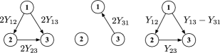
Figure 1: The two leftmost DAGs occur with probability $\frac{1}{2}$, yielding the difference graph $G_{\mu}$ at right, assuming $Y_{23}>Y_{32}$.

Definition 4.

The measure $\mu$ on a set $Y$ of adjacency matrices is low-noise when the corresponding difference graph $G_{\mu}$ satisfies the following reverse triangle inequality: whenever there is an edge $({i}\rightarrow{j})$ and an edge $({j}\rightarrow{k})$ in $G_{\mu}$, the weight $Y_{ik}^{\mu}-Y_{ki}^{\mu}$ on the edge $({i}\rightarrow{k})$ is greater than or equal to the path weight $Y^{\mu}_{ij}-Y^{\mu}_{ji}+Y^{\mu}_{jk}-Y^{\mu}_{kj}$ on the path $(i\to j\to k)$.

If $\mu$ satisfies Definition 4, its difference graph $G_{\mu}$ is a DAG. Indeed, the definition ensures that all global preference information in $G_{\mu}$ (the sum of weights along any path) conforms with and reinforces local preference information (the weight on a single edge). Hence, we would expect any reasonable ranking method to be consistent in this setting. Nevertheless, typical pairwise surrogate losses are inconsistent in this low-noise setting (see also the weaker Theorem 11 in our preliminary work DuchiMaJo10 ):

Theorem 2

Let $\varphi$ be a loss of the form (12) and assume $h(0)=0$. If $\phi$ is convex, then even in the low-noise setting of Definition 4 the loss $\varphi$ is not structure-consistent.

Given the difficulties we encounter using losses of the form (12), it is reasonable to consider a reformulation of the surrogate. A natural alternative is a margin-based loss, which encodes a desire to separate ranking scores by large margins dependent on the preferences in a graph. Similar losses have been proposed, for example, by ShashuaLe02 . The next result shows that convex margin-based losses are also inconsistent, even in low-noise settings. (See also the weaker Theorem 12 of our preliminary work DuchiMaJo10 .)

Theorem 3

Let $h\dvtx\mathbb{R}\rightarrow\mathbb{R}$ and $\varphi$ be a loss of the form

$$\varphi(\alpha,Y)=\sum_{i,j:Y_{ij}>0}\phi\bigl{(}\alpha_{i}-\alpha_{j}-h(Y_{ij})\bigr{)}.$$ (13)

If $\phi$ is convex, then even in the low-noise setting of Definition 4 the loss $\varphi$ is not structure-consistent.

3.3 Achieving Fisher consistency

Although Section 3.2 suggests an inherent difficulty in the development of tractable losses for ranking, tractable Fisher consistency is in fact achievable if one has access to complete preference data. We review a few of the known results here, showing how they follow from the Fisher consistency guarantees in Section 3.1, and derive some new Fisher consistency guarantees for the complete data setting (we defer all proofs to the supplementary material DuchiMaJo13supp ). These results may appear to be of limited practical value, since complete preference judgments are typically unavailable or untrustworthy, but, as we show in Sections 4 and 5, they can be combined with aggregation strategies to yield procedures that are both practical and come with consistency guarantees.

We first define the normalized discounted cumulative gain (NDCG) family of complete data losses. Such losses are common in applications like web search, since they penalize ranking errors at the top of a ranked list more heavily than errors farther down the list. Let $s\in\mathcal{S}\subseteq\mathbb{R}^{m}$ be a vector of relevance scores and $\alpha\in\mathbb{R}^{m}$ be a vector of predicted scores. Define $\pi_{\alpha}$ to be the permutation associated with $\alpha$, so that $\pi_{\alpha}(j)$ is the rank of item $j$ in the ordering induced by $\alpha$. Following Ravikumar et al. RavikumarTeYa11 , a general class of NDCG loss functions can be defined as follows:

$$L(\alpha,s)=1-\frac{1}{Z(s)}\sum_{j=1}^{{m}}\frac{G(s_{j})}{F(\pi_{\alpha}(j))},\qquad Z(s)=\max_{\alpha^{\prime}}\sum_{j=1}^{m}\frac{G(s_{j})}{F(\pi_{\alpha^{\prime}}(j))},$$ (14)

where $G$ and $F$ are functions monotonically increasing in their arguments. By inspection, $L\in[0,1]$, and we remark that the standard NDCG criterion JarvelinKe04 uses $G(s_{j})=2^{s_{j}}-1$ and $F(j)=\log(1+j)$. The “precision at $k$” loss ManningRaSc08 can also be written in the form (14), where $G(s_{j})=s_{j}$ (assuming that $s_{j}\geq 0$) and $F(j)=1$ for $j\leq k$ and $F(j)=+\infty$ otherwise, which measures the relevance of the top $k$ items given by the vector $\alpha$. This form generalizes standard forms of precision, which assume $s_{j}\in\{0,1\}$.

To analyze the consistency of surrogate losses for the NDCG family (14), we first compute the loss $\ell(\alpha,\mu)$ and then state a corollary to Proposition 2. Observe that for any $\mu\in\mathcal{M}(\mathcal{S})$,

$$\ell(\alpha,\mu)=1-\sum_{j=1}^{m}\frac{1}{F(\pi_{\alpha}(j))}\int\frac{G(s_{j})}{Z(s)}\,d\mu(s).$$

Since the function $F$ is increasing in its argument, minimizing $\ell(\alpha,\mu)$ corresponds to choosing any vector $\alpha$ whose values $\alpha_{j}$ obey the same order as the ${m}$ points $\int G(s_{j})/Z(s)\,d\mu(s)$. In particular, the range of $\ell$ is finite for any $\mu$ since it depends only on the permutation induced by $\alpha$, so we have Corollary 1.

Corollary 1

Define the set

$$A(\mu)=\biggl{\{}\alpha\in\mathbb{R}^{m}\mid\alpha_{j}>\alpha_{l}\mbox{ when }\int\frac{G(s_{j})}{Z(s)}\,d\mu(s)>\int\frac{G(s_{l})}{Z(s)}\,d\mu(s)\biggr{\}}.$$ (15)

A surrogate loss $\varphi$ is Fisher-consistent for the NDCG family (14) if and only if for all $\mu\in\mathcal{M}(\mathcal{S})$,

$$\inf_{\alpha}\Bigl{\{}\ell_{\varphi}(\alpha,\mu)-\inf_{\alpha^{\prime}}\ell_{\varphi}\bigl{(}\alpha^{\prime},\mu\bigr{)}\mid\alpha\notin A(\mu)\Bigr{\}}>0.$$

Corollary 1 recovers the main flavor of the consistency results in the papers of Ravikumar et al. RavikumarTeYa11 and Buffoni et al. BuffoniCaGaUs11 . The surrogate $\varphi$ is consistent if and only if it preserves the order of the integrated terms $\int G(s_{j})/Z(s)\,d\mu(s)$: any sequence $\alpha_{n}$ tending to the infimum of $\ell_{\varphi}(\alpha,\mu)$ must satisfy $\alpha_{n}\in A(\mu)$ for large enough $n$. Zhang Zhang04a presents several examples of such losses; as a corollary to his Theorem 5 (also noted by BuffoniCaGaUs11 ), the loss

$$\varphi(\alpha,s):=\sum_{j=1}^{m}\frac{G(s_{j})}{Z(s)}\sum_{l=1}^{m}\phi(\alpha_{l}-\alpha_{j})$$

is convex and structure-consistent (in the sense of Definition 3) whenever $\phi\dvtx\mathbb{R}\rightarrow\mathbb{R}_{+}$ is nonincreasing, differentiable and satisfies $\phi^{\prime}(0)<0$. The papers RavikumarTeYa11 , BuffoniCaGaUs11 contain more examples and a deeper study of NDCG losses. To extend Corollary 1 to a uniform result, we note that if $G(s_{j})>0$ for all $j$ and $\mathcal{S}$ is compact, then $\varphi$ is 0-coercive over the set $\{\alpha_{1}=0\}$, whence Theorem 1 implies that structure consistency coincides with uniform consistency.

Another family of loss functions is based on a cascade model of user behavior ChapelleMeZhGr09 . These losses model dependency among items or results by assuming that a user scans an ordered list of results from top to bottom and selects the first satisfactory result. Here, satisfaction is determined independently at each position. Let $\pi_{\alpha}^{-1}(i)$ denote the index of item that $\alpha\in\mathbb{R}^{m}$ assigns to rank $i$. The form of such expected reciprocal rank (ERR) losses is

$$L(\alpha,s)=1-\sum_{i=1}^{m}\frac{1}{F(i)}G(s_{\pi_{\alpha}^{-1}(i)})\prod_{j=1}^{i-1}\bigl{(}1-G(s_{\pi_{\alpha}^{-1}(j)})\bigr{)},$$ (16)

where $G\dvtx\mathbb{R}\rightarrow[0,1]$ is a nondecreasing function that indicates the prior probability that a result with score $s_{j}$ is selected, and $F\dvtx\mathbb{N}\rightarrow[{1},{\infty})$ is an increasing function that more heavily weights the first items. The ERR family also satisfies $L\in[0,1]$, and empirically correlates well with user satisfaction in ranking tasks ChapelleMeZhGr09 .

Computing the expected conditional risk $\ell(\alpha,\mu)$ for general $\mu\in\mathcal{M}(\mathcal{S})$ is difficult, but we can compute it when $\mu$ is a product measure over $s_{1},\ldots,s_{m}$. Indeed, in this case, we have

$$\ell(\alpha,\mu) = 1-\sum_{i=1}^{m}\frac{1}{F(i)}\int G(s_{\pi_{\alpha}^{-1}(i)})\prod_{j=1}^{i-1}\bigl{(}1-G(s_{\pi_{\alpha}^{-1}(j)})\bigr{)}\,d\mu(s)$$

$$= 1-\sum_{i=1}^{m}\frac{1}{F(i)}\mathbb{E}_{\mu}\bigl{[}G(s_{\pi_{\alpha}^{-1}(i)})\bigr{]}\prod_{j=1}^{i-1}\bigl{(}1-\mathbb{E}_{\mu}\bigl{[}G(s_{\pi_{\alpha}^{-1}(j)})\bigr{]}\bigr{)}.$$

When one believes that the values $G(s_{i})$ represent the a priori relevance of the result $i$, this independence assumption is not unreasonable, and indeed, in Section 5 we provide examples in which it holds. Regardless, we see that $\ell(\alpha,\mu)$ depends only on the permutation $\pi_{\alpha}$, and we can compute the minimizers of the conditional risk for the ERR family (16) using the following lemma, with proof provided in the supplementary material DuchiMaJo13supp .

Lemma 1

Let $p_{i}=\mathbb{E}_{\mu}[G(s_{i})]$. The permutation $\pi$ minimizing $\ell(\alpha,\mu)$ is in decreasing order of the $p_{i}$.

Lemma 1 shows that an order-preserving property is necessary and sufficient for the Fisher-consistency of a surrogate $\varphi$ for the ERR family (16), as it was for the NDCG family (14). To see this, we apply a variant of Corollary 1 where $A(\mu)$ as defined in equation (15) is replaced with the set

$$A(\mu)=\biggl{\{}\alpha\in\mathbb{R}^{m}\mid\alpha_{j}>\alpha_{l}\mbox{ whenever }\int G(s_{j})\,d\mu(s)>\int G(s_{l})\,d\mu(s)\biggr{\}}.$$

Theorem 5 of Zhang04a implies that $\varphi(\alpha,s)=\sum_{j=1}^{m}G(s_{j})\sum_{l=1}^{m}\phi(\alpha_{l}-\alpha_{j})$ is a consistent surrogate when $\phi$ is convex, differentiable and nonincreasing with $\phi^{\prime}(0)<0$. Theorem 1 also yields an equivalence between structure and uniform consistency under suitable conditions on $\mathcal{S}$.

Before concluding this section, we make a final remark, which has bearing on the aggregation strategies we discuss in Section 5. We have assumed that the structure spaces $\mathcal{S}$ for the NDCG (14) and ERR (16) loss families consist of real-valued relevance scores. This is certainly not necessary. In some situations, it may be more beneficial to think of $s\in\mathcal{S}$ as simply an ordered list of the results or as a directed acyclic graph over $\{1,\ldots,{m}\}$. We can then apply a transformation $r\dvtx\mathcal{S}\rightarrow\mathbb{R}^{m}$ to get relevance scores, using $r(s)$ in place of $s$ in the losses (14) and (16). This has the advantage of causing $\mathcal{S}$ to be finite, so Theorem 1 applies, and there exists a nondecreasing function $\zeta$ with $\zeta(0)=0$ such that for any distribution and any measurable $f$,

$$R(f)-R^{*}\leq\zeta\bigl{(}R_{\varphi}(f)-R_{\varphi}^{*}\bigr{)}.$$

4 Uniform laws and asymptotic consistency

In Section 3, we gave examples of losses based on readily available pairwise data but for which Fisher-consistent tractable surrogates do not exist. The existence of Fisher-consistent tractable surrogates for other forms of data, as in Section 3.3, suggests that aggregation of pairwise and partial data into more complete data structures, such as lists or scores, makes the problem easier. However, it is not obvious how to design statistical procedures based on aggregation. In this section, we formally define a class of suitable estimators that permit us to take advantage of the weak convergence of Assumption A and show that uniform laws of large numbers hold for our surrogate losses. This means that we can indeed asymptotically minimize the risk (3) as desired.

Our aim is to develop an empirical analogue of the population surrogate risk (6) that converges uniformly to the population risk under minimal assumptions on the loss $\varphi$ and structure function $s$. Given a dataset $\{(Q_{i},Y_{i})\}_{i=1}^{n}$ with $(Q_{i},Y_{i})\in\mathcal{Q}\times\mathcal{Y}$, we begin by defining, for each query $q$, the batch of data belonging to the query, $\mathcal{B}(q)=\{i\in\{1,\ldots,n\}\mid Q_{i}=q\}$, and the empirical count of the number of items in the batch, $\widehat{n}_{q}=|\mathcal{B}(q)|$. As a first attempt at developing an empirical objective, we might consider an empirical surrogate risk based on complete aggregation over the batch of data belonging to each query:

$$\frac{1}{n}\sum_{q}\widehat{n}_{q}\varphi\bigl{(}f(q),s\bigl{(}\bigl{\{}Y_{i_{j}}\mid i_{j}\in\mathcal{B}(q)\bigr{\}}\bigr{)}\bigr{)}.$$ (17)

While we would expect this risk to converge uniformly when $\varphi$ is a sufficiently smooth function of its structure argument, the analysis of the complete aggregation risk (17) requires overly detailed knowledge of the surrogate $\varphi$ and the structure function $s$.

To develop a more broadly applicable statistical procedure, we instead consider an empirical surrogate based on $U$-statistics. By trading off the nearness of an order-$k$ $U$-statistic to an i.i.d. sample and the nearness of the limiting structure distribution $\mu_{q}$ to a structure $s(Y_{1},\ldots,Y_{k})$ aggregated over $k$ draws, we can obtain consistency under mild assumptions on $\varphi$ and $s$. More specifically, for each query $q$, we consider the surrogate loss

$$\pmatrix{\widehat{n}_{q}\cr k}^{-1}\mathop{\sum_{i_{1}<\cdots<i_{k},}}_{i_{j}\in\mathcal{B}(q)}\varphi\bigl{(}f(q),s(Y_{i_{1}},\ldots,Y_{i_{k}})\bigr{)}.$$ (18)

When $\widehat{n}_{q}<k$, we adopt the convention ${\widehat{n}_{q}\choose k}=1$, and the above sum becomes the single term $\varphi(f(q),s(\{Y_{i_{j}}\mid i_{j}\in\mathcal{B}(q)\}))$ as in the expression (17). Hence, our $U$-statistic loss recovers the complete aggregation loss (17) when $k=\infty$.

An alternative formulation to loss (18) might consist of $\lceil{|\mathcal{B}(q)|/k}\rceil$ aggregation terms per query, with each query-preference pair appearing in a single term. However, the instability of such a strategy is high: a change in the ordering of the data or a substitution of queries could have a large effect on the final estimator. The $U$-statistic (18) grants robustness to such perturbations in the data. Moreover, by choosing the right rate of increase of the aggregation order $k$ as a function of $n$, we obtain consistent procedures for a broad class of surrogates $\varphi$ and structures $s$.

We associate with the surrogate loss (18) a surrogate empirical risk that weights each query by its empirical probability of appearance:

$$\qquad\widehat{R}_{\varphi,n}(f):=\frac{1}{n}\sum_{q}\widehat{n}_{q}\pmatrix{\widehat{n}_{q}\cr k}^{-1}\mathop{\sum_{i_{1}<\cdots<i_{k},}}_{i_{j}\in\mathcal{B}(q)}\varphi\bigl{(}f(q),s(Y_{i_{1}},\ldots,Y_{i_{k}})\bigr{)}.$$ (19)

Let $\mathbb{P}_{n}$ denote the probability distribution of the queries given that the dataset is of size $n$. Then by iteration of expectation and Fubini’s theorem, the surrogate risk (19) is an unbiased estimate of the population quantity

$$\quad R_{\varphi,n}(f):=\sum_{q}\Biggl{[}\sum_{l=1}^{n}l\mathbb{P}_{n}(\widehat{n}_{q}=l)\mathbb{E}\bigl{[}\varphi\bigl{(}f(Q),s(Y_{1},\ldots,Y_{l\wedge k})\bigr{)}\Bigm{|}Q=q\bigr{]}\Biggr{]}.$$ (20)

It remains to establish a uniform law of large numbers guaranteeing the convergence of the empirical risk (19) to the target population risk (6). Under suitable conditions such as those of Section 3, this ensures the asymptotic consistency of computationally tractable statistical procedures. Hereafter, we assume that we have a nondecreasing sequence of function classes $\mathcal{F}_{n}$, where any $f\in\mathcal{F}_{n}$ is a scoring function for queries, mapping $f\dvtx\mathcal{Q}\rightarrow\mathbb{R}^{m}$ and giving scores to the (at most ${m}$) results for each query $q\in\mathcal{Q}$. Our goal is to give sufficient conditions for the convergence in probability

$$\sup_{f\in\mathcal{F}_{n}}\bigl{|}\widehat{R}_{\varphi,n}(f)-R_{\varphi}(f)\bigr{|}\stackrel{{\scriptstyle p}}{{\rightarrow}}0\qquad\mbox{as }n\rightarrow\infty.$$ (21)

While we do not provide fully general conditions under which the convergence (21) occurs, we provide representative, checkable conditions sufficient for convergence. At a high level, to establish (21), we control the uniform difference between the expectations $R_{\varphi,n}(f)$ and $R_{\varphi}(f)$ and bound the distance between the empirical risk $\widehat{R}_{\varphi,n}$ and its expectation $R_{\varphi,n}$ via covering number arguments. We now specify assumptions under which our results hold, deferring all proofs to the supplementary material DuchiMaJo13supp .

Without loss of generality, we assume that $p_{q}$, the true probability of seeing the query $q$, is nonincreasing in the query index $q$. First, we describe the tails of the query distribution:

Assumption D.

There exist constants $\beta>0$ and $K_{1}>0$ such that $p_{q}\leq K_{1}q^{-\beta-1}$ for all $q$. That is, $p_{q}=\mathcal{O}(q^{-\beta-1})$.

Infinite sets of queries $\mathcal{Q}$ are reasonable, since search engines, for example, receive a large volume of entirely new queries each day. Our arguments also apply when $\mathcal{Q}$ is finite, in which case we can take $\beta\uparrow\infty$.

Our second main assumption concerns the behavior of the surrogate loss $\varphi$ over the function class $\mathcal{F}_{n}$, which we assume is contained in a normed space with norm $\|{\cdot}\|$.

Assumption E ((Bounded Lipschitz losses)).

The surrogate loss function $\varphi$ is bounded and Lipschitz continuous over $\mathcal{F}_{n}$: for any $s\in\mathcal{S}$, any $f,f_{1},f_{2}\in\mathcal{F}_{n}$, and any $q\in\mathcal{Q}$, there exist constants $B_{n}$ and $L_{n}<\infty$ such that

$$0\leq\varphi\bigl{(}f(q),s\bigr{)}\leq B_{n}$$

and

$$\bigl{|}\varphi\bigl{(}f_{1}(q),s\bigr{)}-\varphi\bigl{(}f_{2}(q),s\bigr{)}\bigr{|}\leq L_{n}\|{f_{1}-f_{2}}\|.$$

This assumption is satisfied whenever $\varphi(\cdot,s)$ is convex and $\mathcal{F}_{n}$ is compact [and contained in the interior of the domain of $\varphi(\cdot,s)$] HiriartUrrutyLe96ab . Our final assumption gives control over the sizes of the function classes $\mathcal{F}_{n}$ as measured by their covering numbers. (The $\varepsilon$-covering number of $\mathcal{F}$ is the smallest $N$ for which there are $f^{i}$, $i\leq N$, such that $\min_{i}\|{f^{i}-f}\|\leq\varepsilon$ for any $f\in\mathcal{F}$.)

Assumption F.

For all $\varepsilon>0$, $\mathcal{F}_{n}$ has $\varepsilon$-covering number $N(\varepsilon,n)<\infty$.

With these assumptions in place, we give a few representative conditions that enable us to guarantee uniform convergence (21). Roughly, these conditions control the interaction between the size of the function classes $\mathcal{F}_{n}$ and the order $k$ of aggregation used with $n$ data points. To that end, we let the aggregation order $k_{n}$ grow with $n$. In stating the conditions, we make use of the shorthand $\mathbb{E}_{q}[\varphi(f(q),s(Y_{1:k}))]$ for $\mathbb{E}[\varphi(f(Q),s(Y_{1},\ldots,Y_{k}))\mid Q=q]$.

Condition I.

There exist a $\rho>0$ and constant $C$ such that for all $q\in\mathcal{Q}$, $n\in\mathbb{N}$, $k\in\mathbb{N}$, and $f\in\mathcal{F}_{n}$,

$$\Bigl{|}\mathbb{E}_{q}\bigl{[}\varphi\bigl{(}f(q),s(Y_{1},\ldots,Y_{k})\bigr{)}\bigr{]}-\lim_{k^{\prime}}\mathbb{E}_{q}\bigl{[}\varphi\bigl{(}f(q),s(Y_{1},\ldots,Y_{k^{\prime}})\bigr{)}\bigr{]}\Bigr{|}\leq CB_{n}k^{-\rho}.$$

Additionally, the sequences $B_{n}$ and $k_{n}$ satisfy $B_{n}=o(k_{n}^{\rho})$.

This condition is not unreasonable; when $\varphi$ and $s$ are suitably continuous, we expect $\rho\geq\frac{1}{2}$. We also consider an alternative covering number condition.

Condition I^′.

Sequences $\{\varepsilon_{n}\}\subset\mathbb{R}_{+}$ and $\{k_{n}\}\subset\mathbb{N}$ and an $\varepsilon_{n}$-cover $\mathcal{F}_{n}^{1},\ldots,\mathcal{F}_{n}^{N(\varepsilon_{n},n)}$ of $\mathcal{F}_{n}$ can be chosen such that

$$\max_{i\in\{1,\dots,N(\varepsilon_{n},n)\}}\inf_{f\in\mathcal{F}_{n}^{i}}\biggl{|}R_{\varphi}(f)-\sum_{q}p_{q}\mathbb{E}_{q}\bigl{[}\varphi\bigl{(}f(q),s(Y_{1},\ldots,Y_{k_{n}})\bigr{)}\bigr{]}\biggr{|}+2L_{n}\varepsilon_{n}\rightarrow 0.$$

Condition I^′ is weaker than Condition I, since it does not require uniform convergence over $q\in\mathcal{Q}$. If the function class $\mathcal{F}$ is fixed for all $n$, then the weak convergence of $s(Y_{1},\ldots,Y_{k})$ as in Assumption A guarantees Condition I^′, since $N(\varepsilon,n)=N(\varepsilon,n^{\prime})<\infty$, and we may take $\varepsilon$ arbitrarily small. We require one additional condition, which relates the growth of $k_{n}$, $B_{n}$, and the function classes $\mathcal{F}_{n}$ more directly.

Condition II.

The sequences $k_{n}$ and $B_{n}$ satisfy $k_{n}B_{n}^{{(1+\beta)}/{\beta}}=o(n)$. Additionally, for any fixed $\varepsilon>0$, the sequences satisfy

$$k_{n}B_{n}\biggl{[}\log N\biggl{(}\frac{\varepsilon}{4L_{n}},n\biggr{)}\biggr{]}^{{1}/{2}}=o(\sqrt{n}).$$

By inspection, Condition II is satisfied for any $k_{n}=o(\sqrt{n})$ if the function classes $\mathcal{F}_{n}$ are fixed for all $n$. Similarly, if for all $k\geq k_{0}$, $s(Y_{1},\ldots,Y_{k})=s(Y_{1},\ldots,Y_{k_{0}})$, so $s$ depends only on its first $k_{0}$ arguments, Condition II holds whenever $\max\{B_{n}^{(1+\beta)/\beta},B_{n}^{2}\log N(\varepsilon/4L_{n},n)\}=o(n)$. If the function classes $\mathcal{F}_{n}$ consist of linear functionals represented by vectors $\theta\in\mathbb{R}^{d_{n}}$ in a ball of some finite radius, then $\log N(\varepsilon,n)\approx d_{n}\log\varepsilon^{-1}$, which means that Condition II roughly requires $k_{n}\sqrt{d_{n}/n}\rightarrow 0$ as $n\rightarrow\infty$. Modulo the factor $k_{n}$, this condition is familiar from its necessity in the convergence of parametric statistical problems.

The conditions in place, we come to our main result on the convergence of our $U$-statistic-based empirical loss minimization procedures.

Theorem 4

Assume Condition I or I^′ and additionally assume the growth Condition II. Under Assumptions D, E and F,

$$\sup_{f\in\mathcal{F}_{n}}\bigl{|}\widehat{R}_{\varphi,n}(f)-R_{\varphi}(f)\bigr{|}\stackrel{{\scriptstyle p}}{{\rightarrow}}0\qquad\mbox{as }n\rightarrow\infty.$$

We remark in passing that if Condition II holds, with the change that the $o(\sqrt{n})$ bound is replaced by $O(n^{\rho})$ for some $\rho<\frac{1}{2}$, the conclusion of Theorem 4 can be strengthened to both convergence almost surely and in expectation.

By inspection, Theorem 4 provides our desired convergence guarantee (21). By combining the Fisher-consistent loss families outlined in Section 3.3 with the consistency guarantees provided by Theorem 4, it is thus possible to design statistical procedures that are both computationally tractable—minimizing only convex risks—and asymptotically consistent.

5 Rank aggregation strategies

In this section, we give several examples of practical strategies for aggregating disparate user preferences under our framework. Motivated by the statistical advantages of complete preference data highlighted in Section 3.3, we first present strategies for constructing complete vectors of relevance scores from pairwise preference data. We then discuss a model for the selection or “click” data that arises in web search and information retrieval and show that maximum likelihood estimation under this model allows for consistent ranking. We conclude this section with a brief overview of structured aggregation strategies.

5.1 Recovering scores from pairwise preferences

Here we treat partial preference observations as noisy evidence of an underlying complete ranking and attempt to achieve consistency with respect to a complete preference data loss. We consider three methods that take as input pairwise preferences and output a relevance score vector $s\in\mathbb{R}^{m}$. Such procedures fit naturally into our ranking-with-aggregation framework: the results in Section 3.3 and Section 4 show that a Fisher-consistent loss is consistent for the limiting distribution of the scores $s$ produced by the aggregation procedure. Thus, it is the responsibility of the statistician—the designer of an aggregation procedure—to determine whether the scores accurately reflect the judgments of the population. We present our first example in some detail to show how aggregation of pairwise judgments can lead to consistency in our framework and follow with brief descriptions of alternate aggregation strategies. For an introduction to the design of aggregation strategies for pairwise data, see Tsukida and Gupta TsukidaGu11 as well as the book by David David69 .

Thurstone–Mosteller least squares and skew-symmetric scoring. The first aggregation strategy constructs a relevance score vector $s$ in two phases. First, it aggregates a sequence of observed preference judgments $Y_{i}\in\mathcal{Y}$, provided in any form, into a skew-symmetric matrix $A\in\mathbb{R}^{{m}\times{m}}$ satisfying $A=-A^{\top}$. Each entry $A_{ij}$ encodes the extent to which item $i$ is preferred to item $j$. Given such a skew-symmetric matrix, Thurstone and Mosteller Mosteller51 recommend deriving a score vector $s$ such that $s_{i}-s_{j}\approx A_{ij}$. In practice, one may not observe preference information for every pair of results, so we define a masking matrix $\Omega\in\{0,1\}^{{m}\times{m}}$ with $\Omega=\Omega^{\top}$, $\Omega_{ii}=1$, and $\Omega_{ij}=1$ if and only if preference information has been observed for the pair $i\neq j$. Letting $\circ$ denote the Hadamard product, a natural objective for selecting scores (e.g., Gulliksen56 ) is the least squares objective

$$\qquad\mathop{\mathrm{minimize}}_{x\dvtx x^{\top}{\mathbh{1}}=0}\frac{1}{4}\sum_{i,j}\Omega_{ij}\bigl{(}A_{ij}-(x_{i}-x_{j})\bigr{)}^{2}=\frac{1}{4}\bigl{\|}{\Omega\circ\bigl{(}A-\bigl{(}\mathbh{1}x^{\top}-x\mathbh{1}^{\top}\bigr{)}\bigr{)}}\bigr{\|}_{\mathrm{Fr}}^{2}.$$ (22)

The gradient of the objective (22) is

$$D_{\Omega}x-(\Omega\circ A)\mathbh{1}-\Omega x\qquad\mbox{where }D_{\Omega}:=\operatorname{diag}(\Omega\mathbh{1}).$$

Setting $s=(D_{\Omega}-\Omega)^{\dagger}(\Omega\circ A)\mathbh{1}$ yields the solution to the minimization problem (22), since $D_{\Omega}-\Omega$ is an unnormalized graph Laplacian matrix Chung98 , and therefore $\mathbh{1}^{\top}s=\mathbh{1}^{\top}(D_{\Omega}-\Omega)^{\dagger}(\Omega\circ A)\mathbh{1}=0$.

If $\Omega=\mathbh{1}\mathbh{1}^{\top}$, so that all pairwise preferences are observed, then the eigenvalue decomposition of $D_{\Omega}-\Omega={m}I-\mathbh{1}\mathbh{1}^{\top}$ can be computed explicitly as $V\Sigma V^{\top}$, where $V$ is any orthonormal matrix whose first column is $1/\sqrt{{m}}$, and $\Sigma$ is a diagonal matrix with entries $0$ (once) and ${m}$ repeated ${m}-1$ times. Thus, letting $s_{A}$ and $s_{B}$ denote solutions to the minimization problem (22) with different skew-symmetric matrices $A$ and $B$ and noting that $A\mathbh{1}\perp\mathbh{1}$ since $\mathbh{1}^{\top}A\mathbh{1}=0$, we have the Lipschitz continuity of the solutions $s$ in $A$:

$$\|{s_{A}-s_{B}}\|_{2}^{2}=\bigl{\|}{\bigl{(}{m}I-\mathbh{1}\mathbh{1}^{\top}\bigr{)}^{\dagger}(A-B)\mathbh{1}}\bigr{\|}_{2}^{2}=\frac{1}{{m}^{2}}\bigl{\|}{(A-B)\mathbh{1}}\bigr{\|}_{2}^{2}\leq\frac{1}{{m}}|\!|\!|{A-B}|\!|\!|_{2}^{2}.$$

Similarly, when $\Omega$ is fixed, the score structure $s$ is likewise Lipschitz in $A$ for any norm $|\!|\!|{\cdot}|\!|\!|$ on skew-symmetric matrices.

A variety of procedures are available for aggregating pairwise comparison data $Y_{i}\in\mathcal{Y}$ into a skew-symmetric matrix $A$. One example, the Bradley–Terry–Luce (BTL) model BradleyTe52 , is based upon empirical log-odds ratios. Specifically, assume that $Y_{i}\in\mathcal{Y}$ are pairwise comparisons of the form $j\succ l$, meaning item $j$ is preferred to item $l$. Then we can set

$$A_{jl}=\log\frac{\widehat{\mathbb{P}}(j\succ l)+c}{\widehat{\mathbb{P}}(j\prec l)+c}\qquad\mbox{for observed pairs }j,l,$$

where $\widehat{\mathbb{P}}$ denotes the empirical distribution over $\{Y_{1},\ldots,Y_{k}\}$ and $c>0$ is a smoothing parameter.

Since the proposed structure $s$ is a continuous function of the skew-symmetric matrix $A$, the limiting distribution $\mu$ is a point mass whenever $A$ converges almost surely, as it does in the BTL model. If aggregation is carried out using only a finite number of preferences rather than letting $k$ approach $\infty$ with $n$, then $\mu$ converges to a nondegenerate distribution. Theorem 1 grants uniform consistency since the score space $\mathcal{S}$ is finite.

Borda count and budgeted aggregation. The Borda count Borda1781 provides a computationally efficient method for computing scores from election results. In a general election setting, the procedure counts the number of times that a particular item was rated as the best, second best, and so on. Given a skew-symmetric matrix $A$ representing the outcomes of elections, the Borda count assigns the scores $s=A\mathbh{1}$. As above, a skew-symmetric matrix $A$ can be constructed from input preferences $\{Y_{1},\ldots,Y_{k}\}$, and the choice of this first-level aggregation can greatly affect the resulting rankings. Ammar and Shah AmmarSh11 suggest that if one has limited computational budget and only pairwise preference information then one should assign to item $j$ the score

$$s_{j}=\frac{1}{{m}-1}\sum_{l\neq j}\widehat{\mathbb{P}}(j\succ l),$$

which estimates the probability of winning an election against an opponent chosen uniformly. This is equivalent to the Borda count when we choose $A_{jl}=\widehat{\mathbb{P}}(j\succ l)-\widehat{\mathbb{P}}(j\prec l)$ as the entries in the skew-symmetric aggregate $A$.

Principal eigenvector method. Saaty Saaty03 describes the principal eigenvector method, which begins by forming a reciprocal matrix $A\in\mathbb{R}^{{m}\times{m}}$, with positive entries $A_{ij}=(A_{ji})^{-1}$, from pairwise comparison judgments. Here $A_{ij}$ encodes a multiplicative preference for item $i$ over item $j$; the idea is that ratios preserve preference strength Saaty03 . To generate $A$, one may use, for example, smoothed empirical ratios $A_{jl}=\frac{\widehat{\mathbb{P}}(j\succ l)+c}{\widehat{\mathbb{P}}(j\prec l)+c}$. Saaty recommends finding a vector $s$ so that $s_{i}/s_{j}\approx A_{ij}$, suggesting using the Perron vector of the matrix, that is, the first eigenvector of $A$.

5.2 Cascade models for selection data

Cascade models CraswellZoTaRa08 , ChapelleMeZhGr09 explain the behavior of a user presented with an ordered list of items, for example from a web search. In a cascade model, a user considers results in the presented order and selects the first to satisfy him or her. The model assumes the result $l$ satisfies a user with probability $p_{l}$, independently of previous items in the list. It is natural to express a variety of ranking losses, including the expected reciprocal rank (ERR) family (16), as expected disutility under a cascade model, but computation and optimization of these losses require knowledge of the satisfaction probabilities $p_{l}$. When the satisfaction probabilities are unknown, Chapelle et al. ChapelleMeZhGr09 recommend plugging in those values $p_{l}$ that maximize the likelihood of observed click data. Here we show that risk consistency for the ERR family is straightforward to characterize when scores are estimated via maximum likelihood.

To this end, fix a query $q$, and let each affiliated preference judgment $Y_{i}$ consist of a triple $({m}_{i},\pi_{i},c_{i})$, where ${m}_{i}$ is the number of results presented to the user, $\pi_{i}$ is the order of the presented results, which maps positions $\{1,\ldots,{m}_{i}\}$ to the full result set $\{1,\ldots,{m}\}$, and $c_{i}\in\{1,\ldots,{m}_{i}+1\}$ is the position clicked on by the user (${m}_{i}+1$ if the user chooses nothing). The likelihood $g$ of an i.i.d. sequence $\{Y_{1},\ldots,Y_{k}\}$ under a cascade model $p$ is

$$g\bigl{(}p,\{Y_{1},\ldots,Y_{k}\}\bigr{)}=\prod_{i=1}^{k}p_{\pi_{i}(c_{i})}^{1({c_{i}\leq m_{i}})}\prod_{j=1}^{c_{i}-1}(1-p_{\pi_{i}(j)}),$$

and the maximum likelihood estimator of the satisfaction probabilities has the closed form

$$\widehat{p}_{l}(Y_{1},\ldots,Y_{k})=\frac{\sum_{i=1}^{k}1({\pi_{i}(c_{i})=l})}{\sum_{i=1}^{k}\sum_{j=1}^{c_{i}}1({\pi_{i}(j)=l})},\qquad l=1,\ldots,{m}.$$

To incorporate this maximum likelihood aggregation procedure into our framework, we define the structure function $s$ to be the vector

$$s(Y_{1},\ldots,Y_{k}):=\widehat{p}(Y_{1},\ldots,Y_{k})\in\mathbb{R}^{m}$$

of maximum likelihood probabilities, and we take as our loss $L$ any member of the ERR family (16). The strong law of large numbers implies the a.s. convergence of $\widehat{p}$ to a vector $p\in[0,1]^{m}$, so that the limiting law $\mu_{q}(\{p\})=1$. Since $\mu_{q}$ is a product measure over $[0,1]^{m}$, Lemma 1 implies that any $\alpha$ inducing the same ordering over results as $p$ minimizes the conditional ERR risk $\ell(\alpha,\mu)$. By application of Theorems 1 (or Proposition 2) and 4, it is possible to asymptotically minimize the expected reciprocal rank by aggregation.

5.3 Structured aggregation

Our framework can leverage aggregation procedures (see, e.g., DworkKuNaSi01 ) that map input preferences into representations of combinatorial objects. Consider the setting of Section 3.2, in which each observed preference judgment $Y$ is the weighted adjacency matrix of a directed acyclic graph, our loss of interest $L$ is the edgewise indicator loss (10), and our candidate surrogate losses have the form (18). Theorems 2 and 3 establish that risk consistency is not generally attainable when $s(Y_{1},\ldots,Y_{k})=Y_{1}$. In certain cases, aggregation can recover consistency. Indeed, define

$$s(Y_{1},\ldots,Y_{k}):=\frac{1}{k}\sum_{i=1}^{k}Y_{i},$$

the average of the input adjacency matrices. For an i.i.d. sequence $Y_{1},Y_{2},\ldots$ associated with a given query $q$, we have $s(Y_{1},\ldots,Y_{n})\stackrel{{\scriptstyle\mathrm{a.s.}}}{{\rightarrow}}\mathbb{E}(Y\mid Q=q)$ by the strong law of large numbers, and hence the asymptotic surrogate risk

$$R_{\varphi}(f)=\sum_{q}p_{q}\int\varphi\bigl{(}f(q),s\bigr{)}\,d\mu_{q}(s)=\sum_{q}p_{q}\varphi\bigl{(}f(q),\mathbb{E}(Y\mid Q=q)\bigr{)}.$$

Recalling the conditional pairwise risk (11), we can rewrite the risk as

$$R(f) = \sum_{q}p_{q}\biggl{[}\sum_{i<j}Y_{ij}^{\mu_{q}}1\bigl{(}{f_{i}(q)\leq f_{j}(q)}\bigr{)}+\sum_{i>j}Y_{ij}^{\mu_{q}}1\bigl{(}{f_{i}(q)<f_{j}(q)}\bigr{)}\biggr{]}$$

$$= \sum_{q}p_{q}\sum_{i>j}\mathbb{E}[Y_{ij}\mid Q=q]$$

$${}+\sum_{q}p_{q}\sum_{i<j}\mathbb{E}[Y_{ij}-Y_{ji}\mid Q=q]1\bigl{(}{f_{i}(q)\leq f_{j}(q)}\bigr{)}.$$

The discussion immediately following Proposition 2 shows that any consistent surrogate $\varphi$ must be bounded away from its minimum for $\alpha\notin\break\operatorname{argmin}_{\alpha^{\prime}}\ell_{\varphi}(\alpha^{\prime},\mu)$. Since the limiting distribution $\mu$ is a point mass at some adjacency matrix $s$ for each $q$, a surrogate loss $\varphi$ is consistent if and only if

$$\inf_{\alpha}\Bigl{\{}\varphi(\alpha,s)-\inf_{\alpha^{\prime}}\varphi\bigl{(}\alpha^{\prime},s\bigr{)}\mid\alpha\notin\mathop{\operatorname{argmin}}_{\alpha^{\prime}}L\bigl{(}\alpha^{\prime},s\bigr{)}\Bigr{\}}>0.$$

In the important special case when the difference graph $G_{\mu}$ associated with $\mathbb{E}[Y\mid Q=q]$ is a DAG for each query $q$ (recall Section 3.2.2), structure consistency is obtained if for each $\alpha^{*}\in\operatorname{argmin}_{\alpha}\varphi(\alpha,s)$, $\operatorname{sign}(\alpha_{i}^{*}-\alpha_{j}^{*})=\operatorname{sign}(s_{ij}-s_{ji})$ for each pair of results $i,j$. As an example, in this setting

$$\varphi(\alpha,s):=\sum_{i,j}[{s_{ij}-s_{ji}}]_{+}\phi(\alpha_{i}-\alpha_{j})$$ (23)

is consistent when $\phi$ is nonincreasing, convex, and has derivative $\phi^{\prime}(0)<0$.

The Fisher-consistent loss (23) is similar to the inconsistent losses (12) considered in Section 3.2, but the coefficients adjoining each $\phi(\alpha_{i}-\alpha_{j})$ summand exhibit a key difference. While the inconsistent losses employ coefficients based solely on the average $i\to j$ weight $s_{ij}$, the consistent loss coefficients are nonlinear functions of the edge weight differences $s_{ij}-s_{ji}$: they are precisely the edge weights of the difference graph $G_{\mu}$ introduced Section 3.2.2. Since at least one of the two coefficients $[s_{ij}-s_{ji}]_{+}$ and $[s_{ji}-s_{ij}]_{+}$ is always zero, the loss (23) penalizes misordering either edge $i\to j$ or $j\to i$. This contrasts with the inconsistent surrogates of Section 3.2, which simultaneously associate nonzero convex losses with opposing edges $i\to j$ and $j\to i$. Note also that our argument for the consistency of the loss (23) does not require Definition 4’s low-noise assumption: consistency holds under the weaker condition that, on average, a population’s preferences are acyclic.

6 Experimental study and implementation

In this section, we describe strategies for solving the convex programs that emerge from our aggregation approach to ranking and demonstrate the empirical utility of our proposed procedures. We begin with a broad description of implementation strategies and end with a presentation of specific experiments.

6.1 Minimizing the empirical risk

At first glance, the empirical risk (19) appears difficult to minimize, since the number of terms grows exponentially in the level of aggregation $k$. Fortunately, we may leverage techniques from the stochastic optimization literature NemirovskiJuLaSh09 , DuchiSi09c to minimize the risk (19) in time linear in $k$ and independent of $n$. Let us consider minimizing a function of the form

$$\widehat{R}_{N}(f):=\frac{1}{N}\sum_{i=1}^{N}\varphi\bigl{(}f,s^{i}\bigr{)}+\Phi(f),$$ (24)

where $\{s^{i}\}_{i=1}^{N}$ is some collection of data, $\varphi(\cdot,s)$ is convex in its first argument, and $\Phi$ is a convex regularizing function (possibly zero).

Duchi and Singer DuchiSi09c , using ideas similar to those of Nemirovski et al. NemirovskiJuLaSh09 , develop a specialized stochastic gradient descent method for minimizing composite objectives of the form (24). Such methods maintain a parameter $f^{t}$, which is assumed to live in convex subset $\mathcal{F}$ of a Hilbert space with inner product $\langle\cdot,\cdot\rangle$, and iteratively update $f^{t}$ as follows. At iteration $t$, an index $i_{t}\in[N]$ is chosen uniformly at random and the gradient $\nabla_{f}\varphi(f^{t},s^{i_{t}})$ is computed at $f^{t}$. The parameter $f$ is then updated via

$$f^{t+1}=\mathop{\operatorname{argmin}}_{f\in\mathcal{F}}\biggl{\{}\bigl{\langle}f,\nabla\varphi\bigl{(}f^{t},s^{i_{t}}\bigr{)}\bigr{\rangle}+\Phi(f)+\frac{1}{2\eta_{t}}\bigl{\|}{f-f^{t}}\bigr{\|}^{2}\biggr{\}},$$ (25)

where $\eta_{t}>0$ is an iteration-dependent stepsize and $\|{\cdot}\|$ denotes the Hilbert norm. The convergence guarantees of the update (25) are well understood NemirovskiJuLaSh09 , DuchiSi09c , DuchiShSiTe10 . Define $\overline{f}^{T}=(1/T)\sum_{t=1}^{T}f^{t}$ to be the average parameter after $T$ iterations. If the function $\widehat{R}_{N}$ is strongly convex—meaning it has at least quadratic curvature—the step-size choice $\eta_{t}\propto 1/t$ gives

$$\mathbb{E}\bigl{[}\widehat{R}_{N}\bigl{(}\overline{f}^{T}\bigr{)}\bigr{]}-\inf_{f\in\mathcal{F}}\widehat{R}_{N}(f)=\mathcal{O}\biggl{(}\frac{1}{T}\biggr{)},$$

where the expectation is taken with respect to the indices $i_{t}$ chosen during each iteration of the algorithm. In the convex case (without assuming any stronger properties than convexity), the step-size choice $\eta_{t}\propto 1/\sqrt{t}$ yields

$$\mathbb{E}\bigl{[}\widehat{R}_{N}\bigl{(}\overline{f}^{T}\bigr{)}\bigr{]}-\inf_{f\in\mathcal{F}}\widehat{R}_{N}(f)=\mathcal{O}\biggl{(}\frac{1}{\sqrt{T}}\biggr{)}.$$

These guarantees also hold with high probability NemirovskiJuLaSh09 , DuchiShSiTe10 .

Neither of the convergence rates $1/T$ or $1/\sqrt{T}$ depends on the number of terms $N$ in the stochastic objective (24). As a consequence, we can apply the composite stochastic gradient method (25) directly to the empirical risk (19): we sample a query $q$ with probability $\widehat{n}_{q}/n$, after which we uniformly sample one of the ${\widehat{n}_{q}\choose k}$ collections $\{i_{1},\ldots,i_{k}\}$ of $k$ indices associated with query $q$, and we then perform the gradient update (25) using the gradient sample $\nabla\varphi(f^{t},s(Y_{i_{1}},\ldots,Y_{i_{k}}))$. This stochastic gradient scheme means that we can minimize the empirical risk in a number of iterations independent of both $n$ and $k$; the run-time behavior of the method scales independently of $n$ and depends on $k$ only so much as computing an instantaneous gradient $\nabla\varphi(f,s(Y_{1},\ldots,Y_{k}))$ increases with $k$.

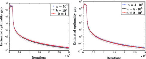
Figure 2: Timing experiments for different values of $k$ and $n$ when applying the method (25). The horizontal axes are the number of stochastic gradient iterations; the vertical axes are the estimated optimality gap for the empirical surrogate risk. Left: varying amount of aggregation $k$, fixed $n=4\cdot 10^{5}$. Right: varying total number of samples $n$, fixed $k=10^{2}$.

In Figure 2, we show empirical evidence that the stochastic method (25) works as described. In particular, we minimize the empirical $U$-statistic-based risk (19) with the loss (28) we employ in our experiments in the next section. In each plot in Figure 2, we give an estimated optimality gap, $\widehat{R}_{\varphi,n}(f^{t})-\inf_{f\in\mathcal{F}}\widehat{R}_{\varphi,n}(f)$, as a function of $t$, the number of iterations. As in the section to follow, $\mathcal{F}$ consists of linear functionals parameterized by a vector $\theta\in\mathbb{R}^{d}$ with $d=136$. To estimate $\inf_{f\in\mathcal{F}}$, we perform 100,000 updates of the procedure (25), then estimate $\inf_{f\in\mathcal{F}}\widehat{R}_{\varphi,n}(f)$ using the output predictor $\widehat{f}$ evaluated on an additional (independent) 50,000 samples (the number of terms in the true objective is too large to evaluate). To estimate the risk $\widehat{R}_{\varphi,n}(f^{t})$, we use a moving average of the previous 100 sampled losses $\varphi(f^{\tau},s^{i_{\tau}})$ for $\tau\in\{t-99,\ldots,t\}$, which is an unbiased estimate of an upper bound on the empirical risk $\widehat{R}_{\varphi,n}(f^{t})$ (see, e.g., CesaBianchiCoGe02 ). We perform the experiment 20 times and plot averages as well as 90% confidence intervals. As predicted by our theoretical results, the number of iterations to attain a particular accuracy is essentially independent of $n$ and $k$; all the plots lie on one another.

6.2 Experimental evaluation

To perform our experimental evaluation, we use a subset of the Microsoft Learning to Rank Web10K dataset QinLiDiXuLi11 , which consists of 10,000 web searches (queries) issued to the Microsoft Bing search engine, a set of approximately 100 potential results for each query, and a relevance score $r\in\mathbb{R}$ associated with each query/result pair. A query/result pair is represented by a $d=136$-dimensional feature vector of standard document-retrieval features.

To understand the benefits of aggregation and consistency in the presence of partial preference data, we generate pairwise data from the observed query/result pairs, so that we know the true asymptotic generating distribution. We adopt a loss $L$ from the NDCG-family (14) and compare three surrogate losses: a Fisher-consistent regression surrogate based on aggregation, an inconsistent but commonly used pairwise logistic loss DekelMaSi03 , and a Fisher-consistent loss that requires access to complete preference data RavikumarTeYa11 . Recalling the NDCG score (14) of a prediction vector $\alpha\in\mathbb{R}^{m}$ for scores $s\in\mathbb{R}^{m}$ (where $\pi_{\alpha}$ is the permutation induced by $\alpha$), we have the loss

$$L(\alpha,s)=1-\frac{1}{Z(s)}\sum_{j=1}^{m}\frac{G(s_{j})}{F(\pi_{\alpha}(j))},$$

where $Z(s)$ is the normalizing value for the NDCG score, and $F(\cdot)$ and $G(\cdot)$ are increasing functions.

Given a set of queries $q$ and relevance scores $r_{i}\in\mathbb{R}$, we generate $n$ pairwise preference observations according to a Bradley–Terry–Luce (BTL) model BradleyTe52 . That is, for each observation, we choose a query $q$ uniformly at random and then select a uniformly random pair $(i,j)$ of results to compare. The pair is ordered as $i\succ j$ (item $i$ is preferred to $j$) with probability $p_{ij}$, and $j\succ i$ with probability $1-p_{ij}=p_{ji}$, where

$$p_{ij}=\frac{\exp(r_{i}-r_{j})}{1+\exp(r_{i}-r_{j})}$$ (26)

for $r_{i}$ and $r_{j}$ the respective relevances of results $i$ and $j$ under query $q$.

We define our structure functions $s_{k}$ as score vectors in $\mathbb{R}^{m}$, where given a set of $k$ preference pairs, the score for item $i$ is

$$s_{k}(i)=\frac{1}{{m}-1}\sum_{j\neq i}\log\frac{\widehat{\mathbb{P}}(j\prec i)}{\widehat{\mathbb{P}}(j\succ i)},$$

the average empirical log-odds of result $i$ being preferred to any other result. Under the BTL model (26), as $k\to\infty$ the structural score converges foreach $i\in[{m}]$ to

$$s(i)=\frac{1}{{m}-1}\sum_{j\neq i}\bigl{[}\log\bigl{(}1+\exp(r_{i}-r_{j})\bigr{)}-\log\bigl{(}1+\exp(r_{j}-r_{i})\bigr{)}\bigr{]}.$$ (27)

In our setting, we may thus evaluate the asymptotic NDCG risk of a scoring function $f$ by computing the asymptotic scores (27). In addition, Corollary 1 shows that if all minimizers of a loss obey the ordering of the values

$$\int_{\mathcal{S}}\frac{G(s(j))}{Z(s)}\,d\mu(s),\qquad j\in\{1,\ldots,{m}\}$$

then the loss is Fisher-consistent. A well-known example CossockZh08 , RavikumarTeYa11 of such a loss is the least-squares loss, where the regression labels are $G(s(j))/Z(s)$:

$$\varphi(\alpha,s)=\frac{1}{2{m}}\sum_{j=1}^{m}\biggl{(}\alpha_{j}-\frac{G(s(j))}{Z(s)}\biggr{)}^{2}.$$ (28)

We compare the least-squares aggregation loss with a pairwise logistic loss natural for the pairwise data generated according to the BTL model (26). Specifically, given a data pair with $i\succ j$, the logistic surrogate loss is

$$\varphi(\alpha,i\succ j)=\log\bigl{(}1+\exp(\alpha_{j}-\alpha_{i})\bigr{)},$$ (29)

which is equivalent or similar to previous losses used for pairwise data in the ranking literature Joachims02 , DekelMaSi03 . For completeness, we also compare with a Fisher-consistent surrogate that requires access to complete preference information in the form of the asymptotic structure scores (27). Following Ravikumar et al. RavikumarTeYa11 , we obtain such a surrogate by granting the regression loss (28) direct access to the asymptotic structure scores. Note that such a construction would be infeasible in any true pairwise data setting.

Having described our sampling procedure, aggregation strategy, and loss functions, we now describe our model. We let $x^{q}_{i}$ denote the feature vector for the $i$th result from query $q$, and we model the scoring function $f(q)_{i}=\langle\theta,x^{q}_{i}\rangle$ for a vector $\theta\in\mathbb{R}^{d}$. For the regression loss (28), we minimize the $U$-statistic-based empirical risk (19) over a variety of orders $k$, while for the pairwise logistic loss (29), we minimize the empirical risk over all pairs sampled according to the BTL model (26). We regularize our estimates by adding $\Phi(\theta)=(\lambda/2)\|{\theta}\|_{2}^{2}$ to the objective minimized, and we use the specialized stochastic method (25) to minimize the empirical risk.

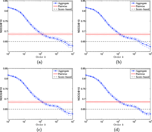
Figure 3: NDCG risk and 95% confidence intervals for $\theta$ estimated using the logistic pairwise loss (29) and the $U$-statistic empirical risk with $\varphi$ chosen to be regression loss (28). The horizontal axis of each plot is the order $k$ of the aggregation in the $U$-statistic (19), the vertical axis is the NDCG risk, and each plot corresponds to a different number $n$ of samples. (a) $n=2\cdot 10^{5}$; (b) $n=4\cdot 10^{5}$; (c) $n=8\cdot 10^{5}$; (d) $n=1.6\cdot 10^{6}$.

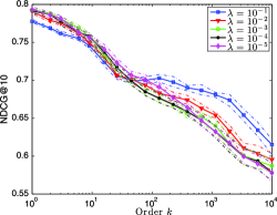
Figure 4: NDCG risk and 95% confidence intervals for $\theta$ estimated using the $U$-statistic empirical risk (19) with $\varphi$ chosen as the regression loss (28) under various choices of the regularization parameter, $\lambda$.

Our goals in the experiments are to understand the behavior of the empirical risk minimizer as the order $k$ of the aggregating statistic is varied and to evaluate the extent to which aggregation improves the estimated scoring function. A secondary concern is to verify that the method is insensitive to the amount $\lambda$ of regularization performed on $\theta$. We run each experiment 50 times and report confidence intervals based on those 50 experiments.

Let $\theta^{\mathrm{reg}}_{n,k}$ denote the estimate of $\theta$ obtained from minimizing the empirical risk (19) with the regression loss (28) on $n$ samples with aggregation order $k$, let $\theta^{\mathrm{log}}_{n}$ denote the estimate of $\theta$ obtained from minimizing the empirical pairwise logistic loss (29), and let $\theta^{\mathrm{full}}$ denote the estimate of $\theta$ obtained from minimizing the empirical risk with surrogate loss (28) using the asymptotic structure scores (27) directly. Then each plot of Figure 3 displays the risk $R(\theta^{\mathrm{reg}}_{n,k})$ as a function of the aggregation order $k$, using $R(\theta^{\mathrm{log}}_{n})$ and $R(\theta^{\mathrm{full}})$ as references. The four plots in the figure correspond to different numbers $n$ of data pairs.

Broadly, the four plots in Figure 3 match our theoretical results. Consistently across the plots, we see that for small $k$, it appears there is not sufficient aggregation in the regression-loss-based empirical risk, and for such small $k$ the pairwise logistic loss is better. However, as the order of aggregation $k$ grows, the risk performance of $\theta_{n,k}^{\mathrm{reg}}$ improves. In addition, with larger sample sizes $n$, the difference between the risk of $\theta^{\mathrm{log}}_{n}$ and $\theta^{\mathrm{reg}}_{n,k}$ becomes more pronounced. The second salient feature of the plots is a moderate flattening of the risk $R(\theta^{\mathrm{reg}}_{n,k})$ and widening of the confidence interval for large values of $k$. This seems consistent with the estimation error guarantees in the theoretical results in Lemmas 7 and 10 in the appendices, where the order $k$ being large has an evidently detrimental effect. Interestingly, however, large values of $k$ still yield significant improvements over $R(\theta^{\mathrm{log}}_{n})$. For very large $k$, the improved performance of $\theta^{\mathrm{reg}}_{n,k}$ over $\theta^{\mathrm{full}}$ is a consequence of sampling artifacts and the fact that we use a finite dimensional representation. [By using sufficiently many dimensions $d$, the estimator $\theta^{\mathrm{full}}$ attains zero risk by matching the asymptotic scores (27) directly.]

Figure 4 displays the risk $R(\theta^{\mathrm{reg}}_{n,k})$ for $n=800\mbox{,}000$ pairs, $k=100$, and multiple values of the regularization multiplier $\lambda$ on $\|{\theta}\|_{2}^{2}$. The results, which are consistent across many choices of $n$, suggest that minimization of the aggregated empirical risk (19) is robust to the choice of regularization multiplier.

7 Conclusions

In this paper, we demonstrated both the difficulty and the feasibility of designing consistent, practicable procedures for ranking. By giving necessary and sufficient conditions for the Fisher consistency of ranking algorithms, we proved that many natural ranking procedures based on surrogate losses are inconsistent, even in low-noise settings. To address this inconsistency while accommodating the incomplete nature of typical ranking data, we proposed a new family of surrogate losses, based on $U$-statistics, that aggregate disparate partial preferences. We showed how our losses can fruitfully leverage any well behaved rank aggregation procedure and demonstrated their empirical benefits over more standard surrogates in a series of ranking experiments.

Our work thus takes a step toward bringing the consistency literature for ranking in line with that for classification, and we anticipate several directions of further development. First, it would be interesting to formulate low-noise conditions under which faster rates of convergence are possible for ranking risk minimization (see, e.g., the work of ClemenconLuVa08 , which focuses on the minimization of a single pairwise loss). Additionally, it may be interesting to study structure functions $s$ that yield nonpoint distributions $\mu$ as the number of arguments $k$ grows to infinity. For example, would scaling the Thurstone–Mosteller least-squares solutions (22) by $\sqrt{k}$—to achieve asymptotic normality—induce greater robustness in the empirical minimizer of the $U$-statistic risk (19)? Finally, exploring tractable formulations of other supervised learning problems in which label data is naturally incomplete could be fruitful.

References

- (1) {bincollection}[auto:STB—2013/06/05—13:45:01] \bauthor\bsnmAmmar, \bfnmA.\binitsA. and \bauthor\bsnmShah, \bfnmD.\binitsD. (\byear2011). \btitleRanking: Compare, don’t score. In \bbooktitleThe 49th Allerton Conference on Communication, Control, and Computing. \bpublisherIEEE, \blocationWashington, DC. \bptokimsref \endbibitem
- (2) {bbook}[mr] \bauthor\bsnmArrow, \bfnmKenneth J.\binitsK. J. (\byear1951). \btitleSocial Choice and Individual Values. \bseriesCowles Commission Monograph \bvolume12. \bpublisherWiley, \blocationNew York, NY. \bidmr=0039976 \bptokimsref \endbibitem
- (3) {barticle}[mr] \bauthor\bsnmBartlett, \bfnmPeter L.\binitsP. L., \bauthor\bsnmJordan, \bfnmMichael I.\binitsM. I. and \bauthor\bsnmMcAuliffe, \bfnmJon D.\binitsJ. D. (\byear2006). \btitleConvexity, classification, and risk bounds. \bjournalJ. Amer. Statist. Assoc. \bvolume101 \bpages138–156. \biddoi=10.1198/016214505000000907, issn=0162-1459, mr=2268032 \bptokimsref \endbibitem
- (4) {bbook}[mr] \bauthor\bsnmBen-Tal, \bfnmAharon\binitsA. and \bauthor\bsnmNemirovski, \bfnmArkadi\binitsA. (\byear2001). \btitleLectures on Modern Convex Optimization: Analysis, Algorithms, and Engineering Applications. \bpublisherSIAM, \blocationPhiladelphia, PA. \biddoi=10.1137/1.9780898718829, mr=1857264 \bptokimsref \endbibitem
- (5) {barticle}[mr] \bauthor\bsnmBradley, \bfnmRalph Allan\binitsR. A. and \bauthor\bsnmTerry, \bfnmMilton E.\binitsM. E. (\byear1952). \btitleRank analysis of incomplete block designs. I. The method of paired comparisons. \bjournalBiometrika \bvolume39 \bpages324–345. \bidissn=0006-3444, mr=0070925 \bptokimsref \endbibitem
- (6) {bincollection}[auto:STB—2013/06/05—13:45:01] \bauthor\bsnmBuffoni, \bfnmD.\binitsD., \bauthor\bsnmCalauzenes, \bfnmC.\binitsC., \bauthor\bsnmGallinari, \bfnmP.\binitsP. and \bauthor\bsnmUsunier, \bfnmN.\binitsN. (\byear2011). \btitleLearning scoring functions with order-preserving losses and standardized supervision. In \bbooktitleProceedings of the 28th International Conference on Machine Learning \bpages825–832. \bpublisherOmnipress, \blocationMadison, WI. \bptokimsref \endbibitem
- (7) {bincollection}[auto:STB—2013/06/05—13:45:01] \bauthor\bsnmCesa-Bianchi, \bfnmN.\binitsN., \bauthor\bsnmConconi, \bfnmA.\binitsA. and \bauthor\bsnmGentile, \bfnmC.\binitsC. (\byear2002). \btitleOn the generalization ability of on-line learning algorithms. In \bbooktitleAdvances in Neural Information Processing Systems 14 \bpages359–366. \bpublisherMIT Press, \blocationCambridge, MA. \bptokimsref \endbibitem
- (8) {bincollection}[auto:STB—2013/06/05—13:45:01] \bauthor\bsnmChapelle, \bfnmO.\binitsO., \bauthor\bsnmMetzler, \bfnmD.\binitsD., \bauthor\bsnmZhang, \bfnmY.\binitsY. and \bauthor\bsnmGrinspan, \bfnmP.\binitsP. (\byear2009). \btitleExpected reciprocal rank for graded relevance. In \bbooktitleConference on Information and Knowledge Management. \bpublisherACM, \blocationNew York. \bptokimsref \endbibitem
- (9) {bbook}[mr] \bauthor\bsnmChung, \bfnmFan R. K.\binitsF. R. K. (\byear1997). \btitleSpectral Graph Theory. \bseriesCBMS Regional Conference Series in Mathematics \bvolume92. \bpublisherConference Board of the Mathematical Sciences, \blocationWashington, DC. \bidmr=1421568 \bptnotecheck year\bptokimsref \endbibitem
- (10) {barticle}[mr] \bauthor\bsnmClémençon, \bfnmStéphan\binitsS., \bauthor\bsnmLugosi, \bfnmGábor\binitsG. and \bauthor\bsnmVayatis, \bfnmNicolas\binitsN. (\byear2008). \btitleRanking and empirical minimization of -statistics. \bjournalAnn. Statist. \bvolume36 \bpages844–874. \biddoi=10.1214/009052607000000910, issn=0090-5364, mr=2396817 \bptokimsref \endbibitem
- (11) {bmisc}[auto:STB—2013/06/05—13:45:01] \bauthor\bsnmCondorcet, \bfnmN.\binitsN. (\byear1785). \bhowpublishedEssai sur l’Application de l’Analyse à la Probabilité des Décisions Rendues à la Pluralité des Voix. Paris. \bptokimsref \endbibitem
- (12) {barticle}[mr] \bauthor\bsnmCossock, \bfnmDavid\binitsD. and \bauthor\bsnmZhang, \bfnmTong\binitsT. (\byear2008). \btitleStatistical analysis of Bayes optimal subset ranking. \bjournalIEEE Trans. Inform. Theory \bvolume54 \bpages5140–5154. \biddoi=10.1109/TIT.2008.929939, issn=0018-9448, mr=2589888 \bptokimsref \endbibitem
- (13) {bincollection}[auto:STB—2013/06/05—13:45:01] \bauthor\bsnmCraswell, \bfnmN.\binitsN., \bauthor\bsnmZoeter, \bfnmO.\binitsO., \bauthor\bsnmTaylor, \bfnmM. J.\binitsM. J. and \bauthor\bsnmRamsey, \bfnmB.\binitsB. (\byear2008). \btitleAn experimental comparison of click position-bias models. In \bbooktitleWeb Search and Data Mining (WSDM) \bpages87–94. \bpublisherACM, \blocationNew York. \bptokimsref \endbibitem
- (14) {bbook}[auto:STB—2013/06/05—13:45:01] \bauthor\bsnmDavid, \bfnmH. A.\binitsH. A. (\byear1969). \btitleThe Method of Paired Comparisons. \bpublisherCharles Griffin & Company, \blocationLondon. \bptokimsref \endbibitem
- (15) {bmisc}[auto:STB—2013/06/05—13:45:01] \bauthor\bparticlede \bsnmBorda, \bfnmJ. C.\binitsJ. C. (\byear1781). \bhowpublishedMemoire sur les Elections au Scrutin. Histoire de l’Academie Royale des Sciences, Paris. \bptokimsref \endbibitem
- (16) {bincollection}[auto:STB—2013/06/05—13:45:01] \bauthor\bsnmDekel, \bfnmO.\binitsO., \bauthor\bsnmManning, \bfnmC.\binitsC. and \bauthor\bsnmSinger, \bfnmY.\binitsY. (\byear2004). \btitleLog-linear models for label ranking. In \bbooktitleAdvances in Neural Information Processing Systems \bvolume16. \bptokimsref \endbibitem
- (17) {barticle}[mr] \bauthor\bsnmDuchi, \bfnmJohn\binitsJ. and \bauthor\bsnmSinger, \bfnmYoram\binitsY. (\byear2009). \btitleEfficient online and batch learning using forward backward splitting. \bjournalJ. Mach. Learn. Res. \bvolume10 \bpages2899–2934. \bidissn=1532-4435, mr=2579916 \bptokimsref \endbibitem
- (18) {bmisc}[auto:STB—2013/06/05—13:45:01] \bauthor\bsnmDuchi, \bfnmJ. C.\binitsJ. C., \bauthor\bsnmMackey, \bfnmL.\binitsL. and \bauthor\bsnmJordan, \bfnmM. I.\binitsM. I. (\byear2013). \bhowpublishedSupplement to “The asymptotics of ranking algorithms.” DOI:\doiurl10.1214/13-AOS1142SUPP. \bptokimsref \endbibitem
- (19) {bincollection}[auto:STB—2013/06/05—13:45:01] \bauthor\bsnmDuchi, \bfnmJ. C.\binitsJ. C., \bauthor\bsnmMackey, \bfnmL.\binitsL. and \bauthor\bsnmJordan, \bfnmM. I.\binitsM. I. (\byear2010). \btitleOn the consistency of ranking algorithms. In \bbooktitleProceedings of the 27th International Conference on Machine Learning (ICML-10) (\beditor\binitsJ.\bfnmJ. \bsnmFürnkranz and \beditor\binitsT.\bfnmT. \bsnmJoachims, eds.) \bpages327–334. \bpublisherOmnipress, \baddressMadison, WI. \bptokimsref \endbibitem
- (20) {bincollection}[auto:STB—2013/06/05—13:45:01] \bauthor\bsnmDuchi, \bfnmJ. C.\binitsJ. C., \bauthor\bsnmShalev-Shwartz, \bfnmS.\binitsS., \bauthor\bsnmSinger, \bfnmY.\binitsY. and \bauthor\bsnmTewari, \bfnmA.\binitsA. (\byear2010). \btitleComposite objective mirror descent. In \bbooktitleProceedings of the Twenty Third Annual Conference on Computational Learning Theory. \bptokimsref \endbibitem
- (21) {bincollection}[auto:STB—2013/06/05—13:45:01] \bauthor\bsnmDwork, \bfnmC.\binitsC., \bauthor\bsnmKumar, \bfnmR.\binitsR., \bauthor\bsnmNaor, \bfnmM.\binitsM. and \bauthor\bsnmSivakumar, \bfnmD.\binitsD. (\byear2001). \btitleRank aggregation methods for the web. In \bbooktitleProceedings of the Tenth International Conference on World Wide Web (WWW10) \bpages613–622. \bpublisherACM, \blocationNew York. \bptokimsref \endbibitem
- (22) {barticle}[mr] \bauthor\bsnmFreund, \bfnmYoav\binitsY., \bauthor\bsnmIyer, \bfnmRaj\binitsR., \bauthor\bsnmSchapire, \bfnmRobert E.\binitsR. E. and \bauthor\bsnmSinger, \bfnmYoram\binitsY. (\byear2003). \btitleAn efficient boosting algorithm for combining preferences. \bjournalJ. Mach. Learn. Res. \bvolume4 \bpages933–969. \biddoi=10.1162/1532443041827916, issn=1532-4435, mr=2125342 \bptnotecheck year\bptokimsref \endbibitem
- (23) {barticle}[auto:STB—2013/06/05—13:45:01] \bauthor\bsnmGulliksen, \bfnmH.\binitsH. (\byear1956). \btitleA least squares method for paired comparisons with incomplete data. \bjournalPsychometrika \bvolume21 \bpages125–134. \bptokimsref \endbibitem
- (24) {bmisc}[auto] \bauthor\bsnmHerbrich, \bfnmR.\binitsR., \bauthor\bsnmGraepel, \bfnmT.\binitsT. and \bauthor\bsnmObermayer, \bfnmK.\binitsK. (\byear2000). \bhowpublishedLarge margin rank boundaries for ordinal regression. In Advances in Large Margin Classifiers. MIT Press, Cambridge, MA. \bptokimsref \endbibitem
- (25) {bbook}[auto:STB—2013/06/05—13:45:01] \bauthor\bsnmHiriart-Urruty, \bfnmJ.\binitsJ. and \bauthor\bsnmLemaréchal, \bfnmC.\binitsC. (\byear1996). \btitleConvex Analysis and Minimization Algorithms I & II. \bpublisherSpringer, \blocationNew York. \bptokimsref \endbibitem
- (26) {bbook}[mr] \bauthor\bsnmHopcroft, \bfnmJohn E.\binitsJ. E. and \bauthor\bsnmUllman, \bfnmJeffrey D.\binitsJ. D. (\byear1979). \btitleIntroduction to Automata Theory, Languages, and Computation. \bpublisherAddison-Wesley, \blocationReading, MA. \bidmr=0645539 \bptokimsref \endbibitem
- (27) {barticle}[auto:STB—2013/06/05—13:45:01] \bauthor\bsnmJärvelin, \bfnmK.\binitsK. and \bauthor\bsnmKekäläinen, \bfnmJ.\binitsJ. (\byear2002). \btitleCumulated gain-based evaluation of IR techniques. \bjournalACM Transactions on Information Systems \bvolume20 \bpages422–446. \bptokimsref \endbibitem
- (28) {bincollection}[auto:STB—2013/06/05—13:45:01] \bauthor\bsnmJoachims, \bfnmT.\binitsT. (\byear2002). \btitleOptimizing search engines using clickthrough data. In \bbooktitleProceedings of the ACM Conference on Knowledge Discovery and Data Mining. \bpublisherACM, \blocationNew York. \bptokimsref \endbibitem
- (29) {barticle}[mr] \bauthor\bsnmMallows, \bfnmC. L.\binitsC. L. (\byear1957). \btitleNon-null ranking models. I. \bjournalBiometrika \bvolume44 \bpages114–130. \bidissn=0006-3444, mr=0087267 \bptokimsref \endbibitem
- (30) {bbook}[auto:STB—2013/06/05—13:45:01] \bauthor\bsnmManning, \bfnmC.\binitsC., \bauthor\bsnmRaghavan, \bfnmP.\binitsP. and \bauthor\bsnmSchütze, \bfnmH.\binitsH. (\byear2008). \btitleIntroduction to Information Retrieval. \bpublisherCambridge Univ. Press, \blocationCambridge. \bptokimsref \endbibitem
- (31) {barticle}[auto:STB—2013/06/05—13:45:01] \bauthor\bsnmMiller, \bfnmG.\binitsG. (\byear1956). \btitleThe magic number seven, plus or minus two: Some limits on our capacity for processing information. \bjournalPsychological Review \bvolume63 \bpages81–97. \bptokimsref \endbibitem
- (32) {barticle}[auto:STB—2013/06/05—13:45:01] \bauthor\bsnmMosteller, \bfnmF.\binitsF. (\byear1951). \btitleRemarks on the method of paired comparisons: I. The least squares solution assuming equal standard deviations and equal correlations. \bjournalPsychometrika \bvolume16 \bpages3–9. \bptokimsref \endbibitem
- (33) {barticle}[mr] \bauthor\bsnmNemirovski, \bfnmA.\binitsA., \bauthor\bsnmJuditsky, \bfnmA.\binitsA., \bauthor\bsnmLan, \bfnmG.\binitsG. and \bauthor\bsnmShapiro, \bfnmA.\binitsA. (\byear2009). \btitleRobust stochastic approximation approach to stochastic programming. \bjournalSIAM J. Optim. \bvolume19 \bpages1574–1609. \biddoi=10.1137/070704277, issn=1052-6234, mr=2486041 \bptnotecheck year\bptokimsref \endbibitem
- (34) {bmisc}[auto:STB—2013/06/05—13:45:01] \bauthor\bsnmQin, \bfnmT.\binitsT., \bauthor\bsnmLiu, \bfnmT. Y.\binitsT. Y., \bauthor\bsnmDing, \bfnmW.\binitsW., \bauthor\bsnmXu, \bfnmJ.\binitsJ. and \bauthor\bsnmLi, \bfnmH.\binitsH. (\byear2012). \bhowpublishedMicrosoft learning to rank datasets. Available at http://research.microsoft.com/en-us/projects/mslr/. \bptokimsref \endbibitem
- (35) {bmisc}[auto:STB—2013/06/05—13:45:01] \bauthor\bsnmRavikumar, \bfnmP.\binitsP., \bauthor\bsnmTewari, \bfnmA.\binitsA. and \bauthor\bsnmYang, \bfnmE.\binitsE. (\byear2011). \bhowpublishedOn NDCG consistency of listwise ranking methods. In Proceedings of the 14th International Conference on Artificial Intelligence and Statistics. JMLR Workshop and Conference Proceedings 15 618–626. Society for Artificial Intelligence and Statistics. \bptokimsref \endbibitem
- (36) {barticle}[mr] \bauthor\bsnmSaaty, \bfnmThomas L.\binitsT. L. (\byear2003). \btitleDecision-making with the AHP: Why is the principal eigenvector necessary. \bjournalEuropean J. Oper. Res. \bvolume145 \bpages85–91. \biddoi=10.1016/S0377-2217(02)00227-8, issn=0377-2217, mr=1947158 \bptokimsref \endbibitem
- (37) {barticle}[mr] \bauthor\bsnmSaaty, \bfnmThomas L.\binitsT. L. (\byear2008). \btitleRelative measurement and its generalization in decision making. Why pairwise comparisons are central in mathematics for the measurement of intangible factors. The analytic hierarchy/network process. \bjournalRev. R. Acad. Cienc. Exactas FíS. Nat. Ser. A Math. RACSAM \bvolume102 \bpages251–318. \biddoi=10.1007/BF03191825, issn=1578-7303, mr=2479460 \bptokimsref \endbibitem
- (38) {bmisc}[auto:STB—2013/06/05—13:45:01] \bauthor\bsnmShashua, \bfnmA.\binitsA. and \bauthor\bsnmLevin, \bfnmA.\binitsA. (\byear2002). \bhowpublishedRanking with large margin principle: Two approaches. In Advances in Neural Information Processing Systems 15. \bptokimsref \endbibitem
- (39) {barticle}[pbm] \bauthor\bsnmShiffrin, \bfnmR. M.\binitsR. M. and \bauthor\bsnmNosofsky, \bfnmR. M.\binitsR. M. (\byear1994). \btitleSeven plus or minus two: A commentary on capacity limitations. \bjournalPsychological Review \bvolume101 \bpages357–361. \bidissn=0033-295X, pmid=8022968 \bptokimsref \endbibitem
- (40) {barticle}[mr] \bauthor\bsnmSteinwart, \bfnmIngo\binitsI. (\byear2007). \btitleHow to compare different loss functions and their risks. \bjournalConstr. Approx. \bvolume26 \bpages225–287. \biddoi=10.1007/s00365-006-0662-3, issn=0176-4276, mr=2327600 \bptokimsref \endbibitem
- (41) {barticle}[auto:STB—2013/06/05—13:45:01] \bauthor\bsnmStewart, \bfnmN.\binitsN., \bauthor\bsnmBrown, \bfnmG.\binitsG. and \bauthor\bsnmChater, \bfnmN.\binitsN. (\byear2005). \btitleAbsolute identification by relative judgment. \bjournalPsychological Review \bvolume112 \bpages881–911. \bptokimsref \endbibitem
- (42) {barticle}[auto:STB—2013/06/05—13:45:01] \bauthor\bsnmThurstone, \bfnmL. L.\binitsL. L. (\byear1927). \btitleA law of comparative judgment. \bjournalPsychological Review \bvolume34 \bpages273–286. \bptokimsref \endbibitem
- (43) {bmisc}[auto:STB—2013/06/05—13:45:01] \bauthor\bsnmTsukida, \bfnmK.\binitsK. and \bauthor\bsnmGupta, \bfnmM. R.\binitsM. R. (\byear2011). \bhowpublishedHow to analyze paired comparison data. Technical Report UWEETR-2011-0004, Univ. Washington, Dept. Electrical Engineering. \bptokimsref \endbibitem
- (44) {barticle}[mr] \bauthor\bsnmZhang, \bfnmTong\binitsT. (\byear2004). \btitleStatistical analysis of some multi-category large margin classification methods. \bjournalJ. Mach. Learn. Res. \bvolume5 \bpages1225–1251. \bidissn=1532-4435, mr=2248016 \bptnotecheck year\bptokimsref \endbibitem
- (45) {barticle}[mr] \bauthor\bsnmZhang, \bfnmTong\binitsT. (\byear2004). \btitleStatistical behavior and consistency of classification methods based on convex risk minimization. \bjournalAnn. Statist. \bvolume32 \bpages56–85. \biddoi=10.1214/aos/1079120130, issn=0090-5364, mr=2051001 \bptokimsref \endbibitem