Optimally-Weighted Herding is Bayesian Quadrature

Abstract

Herding and kernel herding are deterministic methods of choosing samples which summarise a probability distribution. A related task is choosing samples for estimating integrals using Bayesian quadrature. We show that the criterion minimised when selecting samples in kernel herding is equivalent to the posterior variance in Bayesian quadrature. We then show that sequential Bayesian quadrature can be viewed as a weighted version of kernel herding which achieves performance superior to any other weighted herding method. We demonstrate empirically a rate of convergence faster than $\mathcal{O}(1/N)$. Our results also imply an upper bound on the empirical error of the Bayesian quadrature estimate.

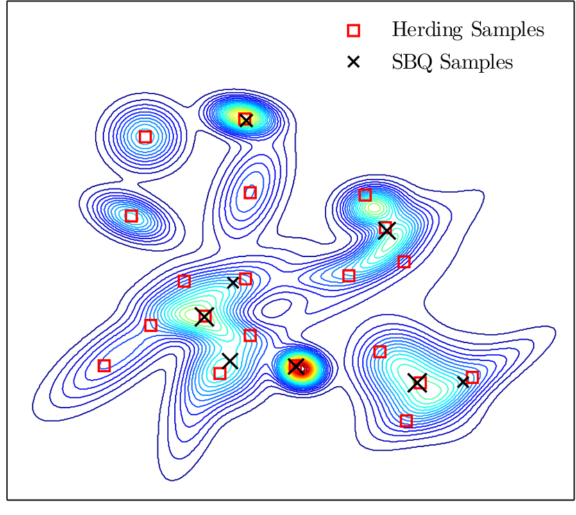
Figure 1: The first 8 samples from sequential Bayesian quadrature, versus the first 20 samples from herding. Only 8 weighted samples are needed to give an estimator with the same maximum mean discrepancy as using 20 herding samples with uniform weights. Relative sizes of samples indicate their relative weights.

1 INTRODUCTION

The problem: Integrals

A common problem in statistical machine learning is to compute expectations of functions over probability distributions of the form:

$$Z_{f,p}=\int f(x)p(x)dx$$ (1)

Examples include computing marginal distributions, making predictions marginalizing over parameters, or computing the Bayes risk in a decision problem. In this paper we assume that the distribution $p(x)$ is known in analytic form, and $f(x)$ can be evaluated at arbitrary locations.

Monte Carlo methods produce random samples from the distribution $p$ and then approximate the integral by taking the empirical mean $\hat{Z}=\frac{1}{N}\sum_{n=1}^{N}f_{x_{n}}$ of the function evaluated at those points. This non-deterministic estimate converges at a rate $\mathcal{O}(\frac{1}{\sqrt{N}})$. When exact sampling from $p$ is impossible or impractical, Markov chain Monte Carlo (MCMC) methods are often used. MCMC methods can be applied to almost any problem but convergence of the estimate depends on several factors and is hard to estimate (CowlesCarlin96). The focus of this paper is on quasi-Monte Carlo methods that – instead of sampling randomly – produce a set of pseudo-samples in a deterministic fashion. These methods operate by directly minimising some sort of discrepancy between the empirical distribution of pseudo-samples and the target distribution. Whenever these methods are applicable, they achieve convergence rates superior to the $\mathcal{O}(\frac{1}{\sqrt{N}})$ rate typical of random sampling.

In this paper we highlight and explore the connections between two deterministic sampling and integration methods: Bayesian quadrature () (BZHermiteQuadrature; BZMonteCarlo) (also known as Bayesian Monte Carlo) and kernel herding (chen2010super). Bayesian quadrature estimates integral (1) by inferring a posterior distribution over $f$ conditioned on the observed evaluations $f_{x_{n}}$, and then computing the posterior expectation of $Z_{f,p}$. The points where the function should be evaluated can be found via Bayesian experimental design, providing a deterministic procedure for selecting sample locations.

Herding, proposed recently by chen2010super, produces pseudosamples by minimising the discrepancy of moments between the sample set and the target distribution. Similarly to traditional Monte Carlo, an estimate is formed by taking the empirical mean over samples $\hat{Z}=\frac{1}{N}\sum_{n=1}^{N}f_{x_{n}}$. Under certain assumptions, herding has provably fast, $\mathcal{O}(\frac{1}{N})$ convergence rates in the parametric case, and has demonstrated strong empirical performance in a variety of tasks.

Summary of contributions

In this paper, we make two main contributions. First, we show that the Maximum Mean Discrepancy (MMD) criterion used to choose samples in kernel herding is identical to the expected error in the estimate of the integral $Z_{f,p}$ under a Gaussian process prior for $f$. This expected error is the criterion being minimized when choosing samples for Bayesian quadrature. Because Bayesian quadrature assigns different weights to each of the observed function values $f({x})$, we can view Bayesian quadrature as a weighted version of kernel herding. We show that these weights are optimal in a minimax sense over all functions in the Hilbert space defined by our kernel. This implies that Bayesian quadrature dominates uniformly-weighted kernel herding and other non-optimally weighted herding in rate of convergence.

Second, we show that minimising the MMD, when using weights is closely related to the sparse dictionary selection problem studied in (KrauseCevher10), and therefore is approximately submodular with respect to the samples chosen. This allows us to reason about the performance of greedy forward selection algorithms for Bayesian Quadrature. We call this greedy method Sequential Bayesian Quadrature ().

We then demonstrate empirically the relative performance of herding, i.i.d random sampling, and , and demonstrate that attains a rate of convergence faster than $\mathcal{O}(1/N)$.

2 HERDING

Herding was introduced by welling2009herding as a method for generating pseudo-samples from a distribution in such a way that certain nonlinear moments of the sample set closely match those of the target distribution. The empirical mean $\frac{1}{N}\sum_{n=1}^{N}f_{x_{n}}$ over these pseudosamples is then used to estimate integral (1).

2.1 Maximum Mean Discrepancy

For selecting pseudosamples, herding relies on an objective based on the maximum mean discrepancy (MMD;  Sriperumbudur2010). MMD measures the divergence between two distributions, $p$ and $q$ with respect to a class of integrand functions $\mathcal{F}$ as follows:

$${\rm MMD}_{\mathcal{F}}\left(p,q\right)=\sup_{f\in\mathcal{F}}\left|\int f_{x}p(x)dx-\int f_{x}q(x)dx\right|$$ (2)

Intuitively, if two distributions are close in the MMD sense, then no matter which function $f$ we choose from $\mathcal{F}$, the difference in its integral over $p$ or $q$ should be small. A particularly interesting case is when the function class $\mathcal{F}$ is functions of unit norm from a reproducing kernel Hilbert space (RKHS) $\mathcal{H}$. In this case, the MMD between two distributions can be conveniently expressed using expectations of the associated kernel $k(x,x^{\prime})$ only (Sriperumbudur2010):

$$MMD^{2}_{\mathcal{H}}(p,q)= \sup_{\begin{subarray}{c}f\in\mathcal{H}\\ \left\|f\right\|_{\mathcal{H}}=1\end{subarray}}\left|\int f_{x}p(x)dx-\int f_{x}q(x)dx\right|^{2}$$ (3)

$$= \left\|\mu_{p}-\mu_{q}\right\|_{\mathcal{H}}^{2}$$ (4)

$$= \iint k(x,y)p(x)p(y)dxdy$$

$$-2 \iint k(x,y)p(x)q(y)dxdy$$

$$+ \iint k(x,y)q(x)q(y)dxdy,$$ (5)

where in the above formula $\mu_{p}=\int\phi({x})p({x})d{x}\in\mathcal{H}$ denotes the mean element associated with the distribution $p$. For characteristic kernels, such as the Gaussian kernel, the mapping between a distribution and its mean element is bijective. As a consequence ${\rm MMD}_{\mathcal{H}}(p,q)=0$ if and only if $p=q$, making it a powerful measure of divergence.

Herding uses maximum mean discrepancy to evaluate of how well the sample set $\{{x}_{1},\ldots,{x}_{N}\}$ represents the target distribution $p$:

$$\epsilon^{2}_{herding} \left(\{{x}_{1},\ldots,{x}_{N}\}\right)={\rm MMD}^{2}_{\mathcal{H}}\left(p,\frac{1}{N}\sum_{n=1}^{N}\delta_{x_{n}}\right)$$ (6)

$$= \iint k(x,y)p(x)p(y)dxdy$$

$$- \frac{1}{N}\sum_{n=1}^{N}\int k(x,x_{n})p(x)dx+\frac{1}{N^{2}}\sum_{n,m=1}^{N}k(x_{n},x_{m})$$ (7)

The herding procedure greedily minimizes its objective $\epsilon_{herding}\left(\{{x}_{1},\ldots,{x}_{N}\}\right)$ , adding pseudosamples ${x}_{n}$ one at a time. When selecting the $n+1$-st pseudosample:

$${x}_{n+1} \leftarrow\operatornamewithlimits{argmin}_{{x}\in\mathcal{X}}\epsilon_{herding}\left(\{{x}_{1},\ldots,{x}_{n},{x}\}\right)$$ (8)

$$=\operatornamewithlimits{argmax}_{{x}\in\mathcal{X}}2\mathbb{E}_{{x}^{\prime}\sim p}\left[{k({x},{x}^{\prime})}\right]-\frac{1}{n+1}\sum_{m=1}^{n}k({x},{x}_{m})\mbox{,}$$

assuming $k({x},{x})=\mbox{const}$. The formula (8) admits an intuitive interpretation: the first term encourages sampling in areas with high mass under the target distribution $p({x})$. The second term discourages sampling at points close to existing samples.

Evaluating (8) requires us to compute $\mathbb{E}_{{x}^{\prime}\sim p}\left[{k({x},{x}^{\prime})}\right]$, that is to integrate the kernel against the target distribution. Throughout the paper we will assume that these integrals can be computed in closed form. Whilst the integration can indeed be carried out analytically in several cases (Song2008; chen2010super), this requirement is the most pertinent limitation on applications of kernel herding, Bayesian quadrature and related algorithms.

2.2 Complexity and Convergence Rates

Criterion (8) can be evaluated in only $\mathcal{O}(n)$ time. Adding these up for all subsequent samples, and assuming that optimisation in each step has $\mathcal{O}(1)$ complexity, producing $N$ pseudosamples via kernel herding costs $\mathcal{O}(N^{2})$ operations in total.

In finite dimensional Hilbert spaces, the herding algorithm has been shown to reduce ${\rm MMD}$ at a rate $\mathcal{O}(\frac{1}{N})$, which compares favourably with the $\mathcal{O}(\frac{1}{\sqrt{N}})$ rate obtained by non-deterministic Monte Carlo samplers. However, as pointed out by bach2012equivalence, this fast convergence is not guaranteed in infinite dimensional Hilbert spaces, such as the RKHS corresponding to the Gaussian kernel.

3 BAYESIAN QUADRATURE

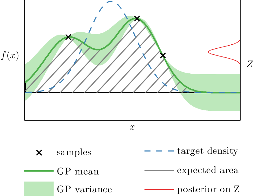
Figure 2: An illustration of Bayesian Quadrature. The function $f(x)$ is sampled at a set of input locations. This induces a Gaussian process posterior distribution on $f$, which is integrated in closed form against the target density, $p({x})$. Since the amount of volume under $f$ is uncertain, this gives rise to a (Gaussian) posterior distribution over $Z_{f,p}$.

So far, we have only considered integration methods in which the integral (1) is approximated by the empirical mean of the function evaluated at some set of samples, or pseudo-samples. Equivalently, we can say that Monte Carlo and herding both assign an equal $\frac{1}{N}$ weight to each of the samples.

In (BZMonteCarlo), an alternate method is proposed: Bayesian Monte Carlo, or Bayesian quadrature (). puts a prior distribution on ${f}$, then estimates integral (1) by inferring a posterior distribution over the function ${f}$, conditioned on the observations ${f}({x}_{n})$ at some query points ${x}_{n}$. The posterior distribution over $f$ then implies a distribution over $Z_{f,p}$. This method allows us to choose sample locations ${x}_{n}$ in any desired manner. See Figure 2 for an illustration of Bayesian Quadrature.

3.1 BQ Estimator

Here we derive the estimate of (1), after conditioning on function evaluations ${f}({x}_{1})\dots f({x}_{N})$, denoted as $f({X})$. The Bayesian solution implies a distribution over $Z_{f,p}$. The mean of this distribution, $\mathbb{E}\left[{Z}\right]$ is the optimal Bayesian estimator for a squared loss.

For simplicity, ${f}$ is assigned a Gaussian process prior with kernel function $k$ and mean $0$. This assumption is very similar to the one made by kernel herding in Eqn. (7).

After conditioning on ${f}_{{x}}$, we obtain a closed-form posterior over ${f}$:

$$p({f}({x}_{\star})|{f}({X}))=\mathcal{N}\!\left({f}_{{x}_{\star}}|\bar{{f}}({x}_{\star}),\operatorname{cov}({x}_{\star},{x}_{\star}^{\prime})\right)$$ (9)

where

$$\bar{{f}}({x}_{\star})= k({x}_{\star},{X})K^{-1}{f}({X})$$ (10)

$$\operatorname{cov}({x}_{\star},{x}_{\star}^{\prime})= k({x}_{\star},{x}^{\prime}_{\star})-k({x}_{\star},{X})K^{-1}k({X},{x}^{\prime}_{\star})$$ (11)

and $K=k({X},{X})$. Conveniently, the posterior allows us to compute the expectation of (1) in closed form:

$$\mathbb{E}_{{\lx@acro@@@def{gp}{gp}{}{{gp}}{{}}}}\left[{Z}\right] =\mathbb{E}_{{\lx@acro@@@def{gp}{gp}{}{{gp}}{{}}}}\left[{\int f({x})p({x})d{x}}\right]$$ (12)

$$=\int\!\!\!\int\!\!f({x})p(f({x})|{f}({X}))p({x})d{x}df$$ (13)

$$=\int\!\!\!\bar{{f}}({x})p({x})d{x}$$ (14)

$$=\left[\int\!\!k({x},{X})p({x})d{x}\right]K^{-1}{f}({X})$$ (15)

$$={\bf{z}}^{T}K^{-1}{f}({X})$$ (16)

where

$$z_{n} =\int\!\!k({x},{x}_{n})p({x})d{x}=\mathbb{E}_{{x}^{\prime}\sim p}\left[{k({x}_{n},{x}^{\prime})}\right].$$ (17)

Conveniently, as in kernel herding, the desired expectation of $Z_{f,p}$ is simply a linear combination of observed function values ${f}({x})$:

$$\mathbb{E}_{{\lx@acro@@@def{gp}{gp}{}{{gp}}{{}}}}\left[{Z}\right] ={\bf{z}}^{T}K^{-1}{f}({X})$$ (18)

$$=\sum_{n}w_{{\lx@acro@@@def{bq}{bq}{}{{bq}}{{}}}}^{(n)}{f}({x}_{n})$$ (19)

where

$$w_{{\lx@acro@@@def{bq}{bq}{}{{bq}}{{}}}}^{(n)} =\sum_{m}{\bf{z}}_{m}^{T}K^{-1}_{mn}$$ (20)

Thus, we can view the BQ estimate as a weighted version of the herding estimate. Interestingly, the weights ${w}_{{\lx@acro@@@def{bq}{bq}{}{{bq}}{{}}}}$ do not need to sum to 1, and are not even necessarily positive.

3.1.1 Non-normalized and Negative Weights

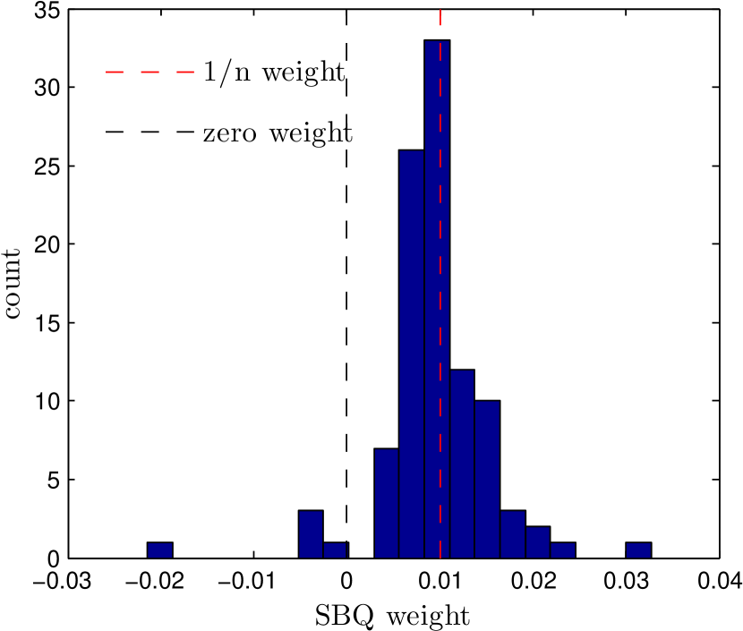
Figure 3: A set of optimal weights given by , after 100 samples were selected on the distribution shown in Figure 1. Note that the optimal weights are spread away from the uniform weight ($\frac{1}{N}$), and that some weights are even negative. The sum of these weights is 0.93.

When weighting samples, it is often assumed, or enforced (as in bach2012equivalence; Song2008), that the weights ${w}$ form a probability distribution. However, there is no technical reason for this requirement, and in fact, the optimal weights do not have this property. Figure 3 shows a representative set of 100 weights chosen on samples representing the distribution in figure 1. There are several negative weights, and the sum of all weights is 0.93.

Figure 4 demonstrates that, in general, the sum of the Bayesian weights exhibits shrinkage when the number of samples is small.

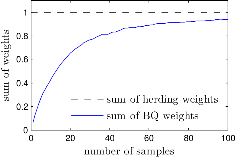
Figure 4: An example of Bayesian shrinkage in the sample weights. In this example, the kernel width is approximately $\nicefrac{{1}}{{20}}$ the width of the distribution being considered. Because the prior over functions is zero mean, in the small sample case the weights are shrunk towards zero. The weights given by simple Monte Carlo and herding do not exhibit shrinkage.

3.2 Optimal sampling for BQ

Bayesian quadrature provides not only a mean estimate of $Z_{f,p}$, but a full Gaussian posterior distribution. The variance of this distribution $\mathbb{V}\left[{Z_{f,p}|f_{x_{1}},\dots,f_{x_{N}}}\right]$ quantifies our uncertainty in the estimate. When selecting locations to evaluate the function $f$, minimising the posterior variance is a sensible strategy. Below, we give a closed form formula for the posterior variance of $Z_{f,p}$, conditioned on the observations $f_{x_{1}}\dots f_{x_{N}}$, which we will denote by $\epsilon^{2}_{{\lx@acro@@@def{bq}{bq}{}{{bq}}{{}}}{}}$. For a longer derivation, see BZMonteCarlo.

$$\epsilon^{2}_{{\lx@acro@@@def{bq}{bq}{}{{bq}}{{}}}{}}({x}_{1},\ldots,{x}_{N}) =\mathbb{V}\left[{Z_{f,p}|f_{x_{1}},\dots,f_{x_{N}}}\right]$$ (21)

$$=\mathbb{E}_{{x},{x}^{\prime}\sim p}\left[{k({x},{x}^{\prime})}\right]-{\bf{z}}^{T}K^{-1}{\bf{z}}\mbox{,}$$ (22)

where ${\bf{z}}_{n}=\mathbb{E}_{{x}^{\prime}\sim p}\left[{k({x}_{n},{x}^{\prime})}\right]$ as before. Perhaps surprisingly, the posterior variance of $Z_{f,p}$ does not depend on the observed function values, only on the location $x_{n}$ of samples. A similar independence is observed in other optimal experimental design problems involving Gaussian processes (guestrin1). This allows the optimal samples to be computed ahead of time, before observing any values of $f$ at all (minka2000dqr).

We can contrast the objective $\epsilon^{2}_{{\lx@acro@@@def{bq}{bq}{}{{bq}}{{}}}{}}$ in (22) to the objective being minimized in herding, $\epsilon^{2}_{herding}$ of equation (7). Just like $\epsilon^{2}_{herding}$, $\epsilon^{2}_{{\lx@acro@@@def{bq}{bq}{}{{bq}}{{}}}{}}$ expresses a trade-off between accuracy and diversity of samples. On the one hand, as samples get close to high density regions under $p$, the values in ${\bf{z}}$ increase, which results in decreasing variance. On the other hand, as samples get closer to each other, eigenvalues of $K$ increase, resulting in an increase in variance.

In a similar fashion to herding, we may use a greedy method to minimise $\epsilon^{2}_{{\lx@acro@@@def{bq}{bq}{}{{bq}}{{}}}{}}$, adding one sample at a time. We will call this algorithm Sequential Bayesian Quadrature ():

$${x}_{n+1} \leftarrow\operatornamewithlimits{argmin}_{{x}\in\mathcal{X}}\epsilon_{{\lx@acro@@@def{bq}{bq}{}{{bq}}{{}}}{}}\left(\{{x}_{1},\ldots,{x}_{n},{x}\}\right)$$ (23)

Using incremental updates to the Cholesky factor, the criterion can be evaluated in $\mathcal{O}(n^{2})$ time. Iteratively selecting $N$ samples thus takes $\mathcal{O}(N^{3})$ time, assuming optimisation can be done on $\mathcal{O}(1)$ time.

4 RELATING $\mathbb{V}\left[{Z_{f,p}}\right]$ TO ${\rm MMD}$

The similarity in the behaviour of $\epsilon^{2}_{herding}$ and $\epsilon^{2}_{{\lx@acro@@@def{bq}{bq}{}{{bq}}{{}}}{}}$ is not a coincidence, the two quantities are closely related to each other, and to MMD.

Proposition 1.

The expected variance in the Bayesian quadrature $\epsilon^{2}_{{\lx@acro@@@def{bq}{bq}{}{{bq}}{{}}}{}}$ is the maximum mean discrepancy between the target distribution $p$ and $q_{{\lx@acro@@@def{bq}{bq}{}{{bq}}{{}}}{}}(x)=\sum_{n=1}^{N}w^{(n)}_{{\lx@acro@@@def{bq}{bq}{}{{bq}}{{}}}{}}\delta_{x_{n}}(x)$

Proof.

The proof involves invoking the representer theorem, using bilinearity of scalar products and the fact that if $f$ is a standard Gaussian process then $\forall g\in\mathcal{H}:\left\langle f,g\right\rangle\sim\mathcal{N}(0,\left\|g\right\|_{\mathcal{H}}^{2})$:

$$\mathbb{V}\left[{Z_{f,p}|f_{x_{1}},\dots,f_{x_{N}}}\right]=$$ (24)

$$=\mathbb{E}_{f\sim GP}\left(\int f(x)p(x)dx-\sum_{n=1}^{N}w^{(n)}_{{\lx@acro@@@def{bq}{bq}{}{{bq}}{{}}}{}}f(x_{n})\right)^{2}$$ (25)

$$=\mathbb{E}_{f\sim GP}\left(\int\left\langle f,\phi(x)\right\rangle p(x)dx-\sum_{n=1}^{N}w^{(n)}_{{\lx@acro@@@def{bq}{bq}{}{{bq}}{{}}}{}}\left\langle f,\phi(x_{n})\right\rangle\right)^{2}$$ (26)

$$=\mathbb{E}_{f\sim GP}\left\langle f,\int\phi(x)p(x)dx-\sum_{n=1}^{N}w^{(n)}_{{\lx@acro@@@def{bq}{bq}{}{{bq}}{{}}}{}}\phi(x_{n})\right\rangle^{2}$$ (27)

$$=\left\|\mu_{p}-\mu_{q_{{\lx@acro@@@def{bq}{bq}{}{{bq}}{{}}}{}}}\right\|_{\mathcal{H}}^{2}$$ (28)

$$={\rm MMD}^{2}(p,q_{{\lx@acro@@@def{bq}{bq}{}{{bq}}{{}}}{}})$$ (29)

∎

We know that the the posterior mean $\mathbb{E}_{{\lx@acro@@@def{gp}{gp}{}{{gp}}{{}}}}\left[{Z_{f,p}|f_{1},\ldots,f_{N}}\right]$ is a Bayes estimator and has therefore the minimal expected squared error amongst all estimators. This allows us to further rewrite $\epsilon^{2}_{{\lx@acro@@@def{bq}{bq}{}{{bq}}{{}}}{}}$ into the following minimax forms:

$$\epsilon^{2}_{{\lx@acro@@@def{bq}{bq}{}{{bq}}{{}}}{}} =\sup_{\begin{subarray}{c}f\in\mathcal{H}\\ \left\|f\right\|_{\mathcal{H}}=1\end{subarray}}\left|\int f_{x}p(x)dx-\sum_{n=1}^{N}w^{(n)}_{{\lx@acro@@@def{bq}{bq}{}{{bq}}{{}}}{}}f_{x_{n}}\right|^{2}$$ (30)

$$=\inf_{\hat{Z}:\mathcal{X}^{N}\mapsto\mathbb{R}}\sup_{\begin{subarray}{c}f\in\mathcal{H}\\ \left\|f\right\|_{\mathcal{H}}=1\end{subarray}}\left|Z-\hat{Z}\left(f_{x_{1}},\ldots,f_{x_{N}}\right)\right|^{2}$$ (31)

$$=\inf_{\bm{w}\in\mathbb{R}^{N}}\sup_{\begin{subarray}{c}f\in\mathcal{H}\\ \left\|f\right\|_{\mathcal{H}}=1\end{subarray}}\left|\int f_{x}p(x)dx-\sum_{n=1}^{N}w_{n}f_{x_{n}}\right|^{2}$$ (32)

Looking at $ϵ{}^2{}_{}$