Convergence, Non-negativity and Stability of a New Milstein Scheme with Applications to Finance

Abstract

We propose and analyse a new Milstein type scheme for simulating stochastic differential equations (SDEs) with highly nonlinear coefficients. Our work is motivated by the need to justify multi-level Monte Carlo simulations for mean-reverting financial models with polynomial growth in the diffusion term. We introduce a double implicit Milstein scheme and show that it possesses desirable properties. It converges strongly and preserves non-negativity for a rich family of financial models and can reproduce linear and nonlinear stability behaviour of the underlying SDE without severe restriction on the time step. Although the scheme is implicit, we point out examples of financial models where an explicit formula for the solution to the scheme can be found.

Key words: Milstein scheme, implicit schemes stochastic differential equation, stability, strong convergence, non-negativity

2000 Mathematics Subject Classification: 60H10, 65J15

1 Introduction

We study numerical approximation of the scalar stochastic differential equation (SDE)

$$dx(t)=f(x(t))dt+g(x(t))dw(t).$$ (1.1)

Here $x(t)\in\mathbb{R}$ for each $t\geq 0$, and, for simplicity, $x(0)$ is taken to be constant. We assume that $f\in C^{1}(\mathbb{R},\mathbb{R})$ and $g\in C^{2}(\mathbb{R},\mathbb{R})$. Throughout we let $(\Omega,{\mathcal{F}},\{{\mathcal{F}}_{t}\}_{t\geq 0},\mathbb{P})$ be a complete probability space with a filtration $\{{\mathcal{F}}_{t}\}_{t\geq 0}$ satisfying the usual conditions, that is, right continuous and increasing while ${\mathcal{F}}_{0}$ contains all $\mathbb{P}$-null sets, and we let $w(t)$ be a Brownian motion defined on the probability space.

Numerical approximations for equation (1.1) are well studied in the case of globally Lipschitz continuous coefficients [17]. Super-linearly growing coefficients, however, raise many new questions. An important example is the Heston stochastic volatility 3/2-model [9, 18]:

$$dx(t)=x(t)(\mu-\alpha x(t))dt+\beta x(t)^{3/2}dw(t),\quad\mu,\alpha,\beta>0.$$ (1.2)

This equation is also known as an inverse square-root process and was shown to be useful for modelling term structure dynamics [1]. We may also view (1.2) as a stochastic extension to the logistic equation [4]. Recently [12] demonstrated that the standard Euler-Maruyama (EM) discretization scheme can diverge in strong and weak senses for SDEs with super-linear coefficients. However, in [26, 27] it is shown that an implicit Euler-type method strongly converges for nonlinearities similar to (1.2). These positive results rely heavily on a one-sided Lipschitz condition satisfied by the drift coefficients of the SDE (1.1), that is, for some constant $K$,

$$(x-y)(f(x)-f(y))\leq K\left|x-y\right|^{2},\quad\hbox{for }x,y\in\mathbb{R}.$$ (1.3)

The solution of (1.2) is non-negative and condition (1.3) holds in the relevant region $x,y\geq 0$. However, in general, numerical approximations do not preserve non-negativity and hence convergence theorems developed in [26, 27] cannot be applied in this situation.

Preservation of positivity is a desirable modeling property, and, in many cases, non-negativity of the numerical approximation is needed in order for the scheme to be well defined. For example, evaluating the diffusion coefficient in (1.2) for a negative argument does not make sense. Many fixes have been proposed in the literature, but these can lead to substantial bias [20]. For more information about positivity preservation we refer the reader to [3, 14, 23, 28]. It was shown in [15] that a class of balanced methods can preserve positivity under an appropriate choice of the weight functions, but strong convergence was proved only under a global Lipschitz condition [21]. Kahl et al. [14] proved that the classical EM scheme does not preserve positivity for any scalar SDE. In the case of the drift implicit EM scheme positivity can be preserved, [28], if the drift coefficient has a very special form, for example as in the Ait-Sahalia interest rate model [2]. It was also shown in [14] that the drift implicit Milstein scheme applied to

$$dx(t)=\alpha(\mu-x(t))dt+\beta x(t)^{p}dw(t)\quad\alpha,\mu,\beta>0,\mathrm{and}\,\,\,p\in[0.5],$$ (1.4)

preserves positivity with no restriction on the time step if $p=0.5$. For $p\in(0.5,1]$ we need to restrict the step size to lie below $\beta^{-2}$.

Higher order approximation carries some pitfalls. It was demonstrated in [10] that Milstein applied to a linear scalar SDE has worse stability properties than EM, even once we allow for implicitness in the drift coefficient. This is undesirable, particularly in the multi-level Monte Carlo (MLMC) setting [5, 6], where we are required to use many simulations with large discretization time step. It is therefore natural to look for more advanced numerical techniques that automatically capture such a property.

In order to address the issues mentioned above, we introduce a new $(\theta,\sigma)$-Milstein scheme for a general scalar SDE. Given any step size $\Delta t$, we define the partition $\mathcal{P}_{\Delta t}:=\{t_{k}=k\Delta t:k=0,1,2,...\}$ of the half line $[0,\infty)$. Letting $X_{t_{k}}$ denote the approximation to $x(t_{k})$, with $X_{t_{0}}=x(0)$ and $\Delta w_{t_{k}}=w(t_{k+1})-w(t_{k})$, the $(\theta,\sigma)$-Milstein-scheme then has the following form

$$X_{t_{k+1}} =X_{t_{k}}+\theta f(X_{t_{k+1}})\Delta t+(1-\theta)f(X_{t_{k}})\Delta t+g(X_{t_{k}})\Delta w_{t_{k}}+\frac{1}{2}L^{1}g(X_{t_{k}})\Delta w_{t_{k}}^{2}$$

$$-\frac{(1-\sigma)}{2}L^{1}g(X_{t_{k}})\Delta t-\frac{\sigma}{2}L^{1}g(X_{t_{k+1}})\Delta t,$$ (1.5)

where $0\leq\theta,\sigma\leq 1$ are free parameters and $L^{1}=g\frac{\partial}{\partial x}$. We note that the $(0,0)$-Milstein scheme reduces to classical Milstein [22]. We will sometimes refer to $(1,1)$-Milstein as the double implicit scheme. The advantage of the extra degree of implicitness offered by $\sigma$ will become clear as we analyse the method. We note that the $(\theta,\sigma)$-Milstein scheme can be naturally derived from the Itô-Stratonovich expansion. Indeed, we can rewrite SDE (1.1) into its Stratonovich form

$$dx(t)=\underline{f}(x(t))dt+g(x(t))\circ dw(t),$$

where $\underline{f}(x)=f(x)-L^{1}g(x)$. In the scalar case the drift-implicit Milstein scheme for the Stratonovich SDE is given by (see [17] p. 345)

$$\bar{X}_{t_{k+1}} =\bar{X}_{t_{k}}+\underline{f}(\bar{X}_{t_{k+1}})\Delta t+g(\bar{X}_{t_{k}})\Delta w_{t_{k}}+\frac{1}{2}L^{1}g(\bar{X}_{t_{k}})\Delta w_{t_{k}}^{2}.$$

Hence, we note that $(\theta,\sigma)$-Milstein may be obtained from the implicit Milstein scheme for a Stratonovich SDE.

In this work, we allow for a nonlinear drift coefficient and show that once $p>0.5$ in (1.4) the step size restriction for non-negativity can be eliminated by the $(\theta,\sigma)$-Milstein method. We also present fairly general conditions for a family of Milstein schemes to preserve positivity. Due to that property the one-sided Lipschitz structure (1.3) will not be lost. Hence, the new scheme can be shown to converge strongly to the solution of the SDE (1.2). Numerically we observe that the rate of strong convergence is $1$, which Giles [5, 6] has shown to be the optimal rate from the MLMC perspective.

The material is structured as follows. Section 2 contains proofs of the existence of positive solutions to (1). In Section 3 we consider stability properties of the double implicit scheme. As motivation we demonstrate that for linear test SDEs we can significantly improve stability properties of the Milstein scheme. We then extend this result to a more general nonlinear setting. In Section 4 we develop the convergence results. We give conclusions in Section 5.

2 Existence of a Solution for the Implicit Schemes

We begin with conditions that guarantee the existence of a unique solution to (1). These will motivate the assumptions that we use to force positivity.

Lemma 2.1.

Let $F$ be a function defined on $\mathbb{R}$ and consider the equation

$$F(x)=b,$$ (2.1)

for a given $b\in\mathbb{R}$. If $F$ is strictly monotone, i.e.,

$$(x-y)(F(x)-F(y))>0,$$ (2.2)

for all $x,y\in\mathbb{R}$, $x\neq y$, then equation (2.1) has at most one solution. If $F$ is continuous and coercive, i.e.,

$$\lim_{\left|x\right|\rightarrow\infty}\frac{xF(x)}{\left|x\right|}=\infty,$$ (2.3)

then for every $b\in\mathbb{R}$, equation (2.1) has a solution $x\in\mathbb{R}$. Moreover, the inverse operator $F^{-1}$ exists.

A proof follows directly from Theorem 26.A in [29]. In order to prove that the $(\theta,\sigma)$-Milstein (1) scheme is well defined we impose two conditions.

Assumption 2.2.

Coefficients $f$ and $g$ in (1.1) are locally Lipschitz continuous and satisfy the following two conditions:
One-sided Lipschitz condition. There exists a constant $K>0$ such that

$$(x-y)(f(x)-f(y))\leq K\left|x-y\right|^{2}\quad\hbox{for all}\quad x,y\in\mathbb{R}.$$ (2.4)

Monotone condition. Operator $L^{1}$ acting on $g$ satisfies

$$(x-y)(L^{1}g(x)-L^{1}g(y))\geq 0\quad\hbox{for all}\quad x,y\in\mathbb{R}.$$ (2.5)

Remark 2.3.

From Assumption 2.2 and the Young inequality we may show that the drift coefficient $f$ satisfies a one-sided Lipschitz-type condition

$$xf(x)\leq K\left|x^{2}\right|+xf(0)\leq a+b\left|x\right|^{2}\quad\hbox{for all}\quad x\in\mathbb{R},$$

where $a=0.5\left|f(0)\right|^{2}$ and $b=(2K+1)/2$. Also from Assumption 2.2 we can show that $xL^{1}g(x)$ is bounded below by a linear function

$$xL^{1}g(x)\geq xL^{1}g(0)\quad\hbox{for all}\quad x,y\in\mathbb{R}.$$ (2.6)

Lemma 2.4.

Define, for any given $\Delta t<(\theta(K+1))^{-1}$,

$$F(x)=x-\theta f(x)\Delta t+\frac{\sigma}{2}L^{1}g(x),\quad x\in\mathbb{R}.$$ (2.7)

Then under Assumption 2.2, for any $b\in\mathbb{R}$ there exists a unique $x\in\mathbb{R}$ such that $F(x)=b$ and hence the method (1) is well defined.

Proof.

In view of Lemma 2.1 it is enough to show that the function $F$ is continuous, coercive and strictly monotone. Clearly, $F(x)$ is continuous on $\mathbb{R}$. By Assumption 2.2,

$$(x-y)(F(x)-F(y))\geq\left|x-y\right|^{2}-\theta K\Delta t\left|x-y\right|^{2}=(1-\theta K\Delta t)\left|x-y\right|^{2}>0,$$

for $\Delta t<(\theta(K+1))^{-1}$. Also by Assumption 2.2 and Remark 2.3

$$xF(x) =x(x-\theta f(x)\Delta t+\frac{\sigma}{2}L^{1}g(x)\Delta t)$$ (2.8)

$$\geq\left|x\right|^{2}(1-\theta\frac{2K+1}{2}\Delta t)-\frac{\theta}{2}x\left|f(0)\right|^{2}\Delta t+\frac{\sigma}{2}xL^{1}g(0)\Delta t,$$

so $F$ is coercive. ∎

From now on we assume that

$$\Delta t<(\theta(K+1))^{-1}$$ (2.9)

2.1 Existence of a Positive Solution for the $(\theta,\sigma)$-Milstein Scheme

In this subsection we introduce assumptions on coefficients $f$ and $g$ of equation (1.1) that allow us to prove the existence of a positive solution to (1).

Definition 2.5.

Given $x(0)>0$, if the solution of (1.1) satisfies $\mathbb{P}(\{x(t)>0:t>0\})=1$ $(\mathbb{P}(\{x(t)\geq 0:t>0\})=1)$, then a stochastic one-step integration scheme computing approximations $X_{t_{k}}\approx x(t_{k})$ preserves positivity (non-negativity) if

$$\mathbb{P}(\{X_{t_{k+1}}>0|X_{t_{k}}>0\})=1\quad(\mathbb{P}(\{X_{t_{k+1}}\geq 0|X_{t_{k}}\geq 0\})=1).$$

Let us note that to use the ideas from Lemma 2.4 to prove the existence of a positive solution to the implicit scheme we need to assume that a one-sided Lipschitz condition on $f$ and monotone condition on $L^{1}g$ hold only on the positive domain. This significantly relaxes the conditions required for the existence and uniqueness of a solution to the implicit scheme (1).

Assumption 2.6.

Coefficients $f$ and $g$ of the equation (1.1) are locally Lipschitz continuous and satisfy the following two conditions:
One-sided Lipschitz condition on $\mathbb{R}_{+}$. There exists a constant $K>0$ such that

$$(x-y)(f(x)-f(y))\leq K\left|x-y\right|^{2}\quad\hbox{for all}\quad x,y\in\mathbb{R}_{+}.$$ (2.10)

Monotone condition on $\mathbb{R}_{+}$. Operator $L^{1}$ acting on $g$ satisfies

$$(x-y)(L^{1}g(x)-L^{1}g(y))\geq 0\quad\hbox{for all}\quad x,y\in\mathbb{R}_{+}.$$ (2.11)

Many mean-reverting models with super- and sub-linear diffusion coefficients satisfy Assumption 2.6; for example, the mean-reverting SDEs

$$dx(t)=(\mu-x(t)^{q})dt+x(t)^{p}dw(t)\quad\hbox{for }x\in\mathbb{R},$$

with $\mu,q>0$ and $p\geq 0.5$.

In general, boundary behavior of one-dimensional SDEs can be fully characterized by the Feller test [16]. Let us consider the interval $(0,\infty)$. We assume that $f$ and $g$ are locally Lipschitz continuous in $(0,\infty)$ and that $g^{2}(x)>0$, for $x\in(0,\infty)$. Let us also define the scale function

$$p(x)=\int_{c}^{x}\exp\left[-2\int_{c}^{s}\frac{f(z)}{g^{2}(z)}dz\right]ds,$$

where $c\in\mathbb{R}$. Since we analyse the behaviour of the above function at $0$, we assume that $c>x$. By Proposition 5.22 in [16] we have that if $p(0+)=-\infty$ then $\mathbb{P}\left[\inf_{0\leq t<\infty}x(t)=0\right]=1$. Therefore, in order to show that the solution to (1.1) is non-negative it is enough to show that $p(0+)=-\infty$.

Assumption 2.7.

The coefficients $f$ and $g$ in (1.1) satisfy the following conditions:

$$f(0)\geq 0,\quad g^{2}(x)>0\;\hbox{for}\;x\in(0,\infty),\;\hbox{and}\;g(0)=0\;\hbox{for}\;x=0.$$

To understand Assumption 2.7 better, we proceed with a heuristic argument. Lets assume that the solution of (1.1) attained $0$ at time $t$. Since the solution is Markovian we can consider the solution to this SDE with initial condition $x(t)=0$ that reads

$$dx(t)=f(0)dt+g(0)dw(t).$$

It is clear that we need to have $g(0)=0$ and $f(0)\geq 0$ in order for $x(t)$ to stay non-negative.

Theorem 2.8.

Let Assumptions 2.6 and 2.7 hold. In addition we require that

$$L^{1}g(x)>0\quad\hbox{for }x>0.$$

Then there exists a unique positive solution to the $(\theta,\sigma)$-Milstein scheme (1) if

$$x-\frac{g^{2}(x)}{2L^{1}g(x)}+(1-\theta)f(x)\Delta t-\frac{(1-\sigma)}{2}L^{1}g(x)\Delta t>\,-\theta f(0)\Delta t,\qquad x>0.$$ (2.12)

Similarly, a unique non-negative solution exists if

$$x-\frac{g^{2}(x)}{2L^{1}g(x)}+(1-\theta)f(x)\Delta t-\frac{(1-\sigma)}{2}L^{1}g(x)\Delta t\geq\,-\theta f(0)\Delta t,\qquad x>0.$$ (2.13)

Proof.

In view of Lemma 2.1 and Definition 2.5 in order to prove the lemma we analyse the following equation

$$F(X_{k+1})=X_{k},\quad\forall k.$$

First we prove that $\mathbb{P}\{X_{k+1}>0\mid X_{k}>0\}=1.$ By Assumptions 2.6 operator $F$ in (2.7) is monotone on $(0,\infty)$ and we have

$$\lim_{x\rightarrow\infty}\frac{xF(x)}{\left|x\right|}=\infty.$$

By Assumption 2.7 we arrive at

$$\lim_{x\rightarrow 0^{+}}\frac{xF(x)}{\left|x\right|}=-\theta f(0)\Delta t.$$

Hence operator $F$ is coercive on $(0,\infty)$. Due to Lemma 2.1, we may complete the proof by showing

$$b(x)=x+(1-\theta)f(x)\Delta t+g(x)\Delta w_{t_{k+1}}+\frac{1}{2}L^{1}g(x)\Delta w_{t_{k+1}}^{2}-\frac{(1-\sigma)}{2}L^{1}g(x)\Delta t>-\theta f(0)\Delta t,\quad\hbox{for}\quad x>0,$$

from which it follows that there exists a positive solution to $F(X_{t_{k+1}})=b(X_{t_{k}})$. First, for any given $x>0$ we find the minimum of the function

$$H(y)=g(x)y+\frac{1}{2}L^{1}g(x)y^{2}.$$

Under the assumption $L^{1}g(x)>0$, for $x>0$, this function possesses a global minimum

$$\min_{y}H(y)=-\frac{g^{2}(x)}{2L^{1}g(x)}.$$

Hence

$$b(x)\geq x+(1-\theta)f(x)\Delta t-\frac{(1-\sigma)}{2}L^{1}g(x)\Delta t-\frac{g^{2}(x)}{2L^{1}g(x)}>-\theta f(0)\Delta t,\quad x>0,$$

as required. For the non-negative case we have $b(x)\geq-\theta f(0)\Delta t$, $x>0$. In that case we also need to check what happens if for some $k$ we have the following event $\{X_{k+1}=0\mid X_{k}>0\}$ (that corresponds to the case where $b(x)=-\theta f(0)\Delta t$ ). Then by Assumption 2.7, $b(0)=(1-\theta)f(0)\Delta t$ and we require that $b(0)\geq-\theta f(0)\Delta t$. That holds due to Assumption 2.7. ∎

For the fully implicit $(1,1)$-Milstein scheme we see from (2.12) that a condition guaranteeing non-negativity independently of $\Delta t$ is

$$x-\frac{g^{2}(x)}{2L^{1}g(x)}\geq 0,\qquad x>0.$$

2.2 Example: Heston Volatility Model

Now we demonstrate that approximation of the $3/2$-Heston volatility model (1.2) with the double implicit Milstein scheme preserves non-negativity. We point out that implicitness in the numerical approximation does not increase computational cost in this case, since we are able to find an explicit solution. This often will be the case in mathematical finance, where typical models have drift and diffusion coefficients of a polynomial type.

The $(1,1)$-Milstein scheme has the form

$$X_{t_{k+1}} =X_{t_{k}}+f(X_{t_{k+1}})\Delta t+g(X_{t_{k}})\Delta w_{t_{k}}+\frac{1}{2}L^{1}g(X_{t_{k}})\Delta w_{t_{k}}^{2}-\frac{1}{2}L^{1}g(X_{t_{k+1}})\Delta t,$$ (2.14)

where now $f(x)=\mu x-\alpha x^{2}$, $g(x)=\beta x^{3/2}$ and $L^{1}g(x)=\frac{3}{2}\beta^{2}x^{2}$. Clearly, the coefficients of equation (1.2) satisfy Assumptions 2.6 and 2.7. Hence, we may show that (2.14) has a unique non-negative solution by verifying condition (2.13) in Theorem 2.8. This reduces to $x-x/3\geq 0$ for $x\geq 0$ and the result follows.

An explicit formula for $X_{t_{k+1}}$ can be found by solving the relevant quadratic equation and choosing the positive solution, to give

$$X_{t_{k+1}}=(2(\alpha+\frac{3}{4}\beta^{2}\Delta t))^{-1}\biggl{(}\sqrt{(1-\mu\Delta t)^{2}+4(\alpha+\frac{3}{4}\beta^{2})\Delta t(X_{t_{k}}+\beta X_{t_{k}}^{3/2}\Delta w_{t_{k}}+3/4\beta^{2}X_{t_{k}}^{2}w^{2}_{t_{k}})}-(1-\mu\Delta t)\biggr{)}.$$

3 Stability Analysis

In this section we examine the global stability of the $(\sigma,\theta)$-Milstein scheme (1). The stability conditions we derive are related to mean-square stability, and we are interested in results that do not put severe restrictions on the time step. We begin with linear test equations where we can derive sharp results and represent stability regions graphically.

3.1 Linear Mean-Square Stability

For the linear test SDE

$$dx(t)=\alpha x(t)dt+\mu x(t)dw(t),$$ (3.1)

the property of mean-square stability,

$$\lim_{t\rightarrow\infty}\mathbb{E}\left|x(t)\right|^{2}=0,$$

is characterized by

$$(2\alpha+\mu^{2})<0.$$ (3.2)

For the $\theta$-Milstein scheme on (3.1),

$$X_{t_{k+1}}=X_{t_{k}}+\theta\alpha X_{t_{k+1}}\Delta t+(1-\theta)\alpha X_{t_{k}}\Delta t+\mu X_{t_{k}}\Delta w_{t_{k+1}}+\frac{1}{2}\mu^{2}X_{t_{k}}[\Delta w_{t_{k+1}}^{2}-\Delta t],$$

the analogous property

$$\lim_{k\rightarrow\infty}\mathbb{E}\left|X_{t_{k}}\right|^{2}=0,$$ (3.3)

was studied in [10]. In particular, the linear stability region

$$R_{MS}:=\{\Delta t\alpha,\Delta t\mu^{2}\in\mathbb{R}:\hbox{method mean-square stable on (\ref{eq:testSDE})}\}$$ (3.4)

was shown to be significantly smaller than that for the corresponding Euler-based scheme. We now examine the new Milstein scheme (1) in this setting, which reduces to

$$X_{t_{k+1}}=X_{t_{k}}+\theta\alpha X_{t_{k+1}}\Delta t+(1-\theta)\alpha X_{t_{k}}\Delta t+\mu X_{t_{k}}\Delta w_{t_{k+1}}$$ (3.5)

$$+\frac{1}{2}\mu^{2}X_{t_{k}}\Delta w_{t_{k+1}}^{2}-\frac{(1-\sigma)}{2}\mu^{2}X_{t_{k}}\Delta t-\frac{\sigma}{2}\mu^{2}X_{t_{k+1}}\Delta t.$$

Theorem 3.1.

The $(\theta,\sigma)$-Milstein scheme (3.5) is linearly mean-square stable, (3.3), if and only if

$$(2\alpha+\mu^{2})+\Delta t\alpha^{2}(1-2\theta)+\frac{\Delta t\mu^{2}}{2}(2\sigma\alpha+\mu^{2})<0.$$ (3.6)

Proof.

We rewrite (3.5) as a recurrence of the form

$$X_{t_{k+1}}=X_{t_{k}}\left(p+q\xi_{t_{k+1}}+r\xi^{2}_{t_{k+1}}\right),$$

where $\xi\sim\mathbb{N}(0,1)$ and

$$p=\frac{1+(1-\theta)\alpha\Delta t-\frac{(1-\sigma)}{2}\mu^{2}\Delta t}{1-\theta\alpha\Delta t+\frac{\sigma}{2}\mu^{2}\Delta t},$$

$$q=\frac{\mu\sqrt{\Delta t}}{1-\theta\alpha\Delta t+\frac{\sigma}{2}\mu^{2}\Delta t},$$

$$r=\frac{\frac{1}{2}\mu^{2}\Delta t}{1-\theta\alpha\Delta t+\frac{\sigma}{2}\mu^{2}\Delta t}.$$

Then

$$\left|X_{t_{k+1}}\right|^{2}=\left|X_{t_{k}}\right|^{2}\left(p^{2}+q^{2}\xi_{t_{k+1}}^{2}+r^{2}\xi^{4}_{t_{k+1}}+2pq\xi_{t_{k+1}}+2pr\xi^{2}_{t_{k+1}}+2qr\xi^{3}_{t_{k+1}}\right).$$

Taking conditional expectation of both sides lead us to

$$\mathbb{E}[\left|X_{t_{k+1}}\right|^{2}|{\cal F}_{t_{k}}]=\left|X_{t_{k}}\right|\left(p^{2}+q^{2}+3r^{2}+2pr\right).$$

Taking conditional expectation of both sides again we obtain

$$\mathbb{E}\left|X_{t_{k+1}}\right|^{2}=\mathbb{E}\left|X_{t_{k}}\right|^{2}\left(p^{2}+q^{2}+3r^{2}+2pr\right).$$ (3.7)

Therefore stability is characterized by $(p+r)^{2}+q^{2}+2r^{2}<1$. This is equivalent to (3.6), as required. ∎

Remark 3.2.

Let us observe that for $\theta=0.5$ and $\sigma=1$ we have recovered precisely the condition (3.2) for the underlying SDE, so the method perfectly reproduces stability for any step-size. More generally, for $\theta\geq 0.5$ and $\sigma=1$ we have the property that “problem stable implies method stable for all $\Delta t$”, which is refered to as A-stability in the deterministic literature.

Motivated by [10, 11] we will draw stability regions for (3.5) in the $x$-$y$ plane, where $x=\alpha\Delta t$ and $y=\mu^{2}\Delta t$. In Figure 1 the stability region of the underyling SDE (3.1) is shaded light grey. The upper pictures in Figure 1 superimpose the stability region of the $(\theta,0)$-Milstein scheme with $\theta=0,0.5,1$, respectively, using darker shading. We see that even in the case of a linear scalar equation we are not able to reproduce the stability region of the underyling test equation (3.1). However, by introducing additional implicitness we overcome this poor performance. The lower pictures in Figure 1 superimpose the stability region of the $(\theta,\sigma)$-Milstein scheme with $(0,1),(0.5,1),(1,1)$, respectively. As stated in Remark 3.2, we recover exactly the stability region of underlying test SDE (3.1) for $\theta=0.5$ and $\sigma=1$.

Figure 1: Light shading: linear mean-square stability of the SDE. Darker shading: linear mean-square stability of Implicit Milstein (upper) and double-implicit Milstein (lower).

3.2 Lyapunov Stability

We begin this section by stating a result that combines Doob’s Decomposition and Martingale Convergence Theorems.

Theorem 3.3 (Lipster and Shiryaev [19]).

Let $Z=\{Z_{n}\}_{n\in\mathbb{N}}$ be a nonnegative decomposable stochastic process with Doob-Meyer decomposition ${Z_{n}}=Z_{0}+A_{n}^{1}-A_{n}^{2}+M_{n}$, where $A^{1}=\{A_{n}^{1}\}_{n\in\mathbb{N}}$ and $A^{1}=\{A_{n}^{1}\}_{n\in\mathbb{N}}$ are a.s. nondecreasing, predictable processes with $A_{0}^{1}=A_{0}^{2}=0$, and $M=\{M_{n}\}_{n\in\mathbb{N}}$ is local $\{{\cal F}_{n}\}_{n\in\mathbb{N}}$-martingale with $M_{0}=0$. Then

$$\left\{\omega:\lim_{n\rightarrow\infty}A^{1}(n)<\infty\right\}\subseteq\left\{\omega:\lim_{n\rightarrow\infty}A^{2}(n)<\infty\right\}\cap\left\{\lim_{n\rightarrow\infty}Z_{n}<\infty\right\}\quad\hbox{a.s.}$$

In [24], the authors proved a very general Stochastic LaSalle Theorem. Here we present a simplified version of their theorem, with fixed Lyapunov function $V(x)=\left|x\right|^{2}$.

Theorem 3.4 (Shen et al. [24]).

Let local Lipschitz conditions hold for $f$ and $g$. Assume further that there exists a function $z\in C(\mathbb{R};\mathbb{R}_{+})$ such that

$$xf(x)+\frac{1}{2}\left|g(x)\right|^{2}\leq-z(x),$$ (3.8)

for all $x\in\mathbb{R}$. For any $x_{0}\in\mathbb{R}$, the solution $(x(t))_{t\geq 0}$ of (1.1) then has the properties that

$$\limsup_{t\rightarrow\infty}\left|x(t)\right|^{2}<\infty\qquad\mathrm{a.s.}\qquad\mathrm{and}\qquad\lim_{t\rightarrow\*}z(x(t))=0\qquad\mathrm{a.s.}$$

Further if $z(x)=0$ if and only if $x=0$, then

$$\lim_{t\rightarrow\infty}x(t)=0\qquad\mathrm{a.s.}\quad\hbox{$\forall$ $x\in\mathbb{R}$}.$$

Now we present a counterpart of this Stochastic LaSalle Theorem for the new Milstein scheme.

Theorem 3.5.

Let Assumption 2.2 hold. Assume that for the $(\theta,\sigma)$-Milstein Scheme (1) there exists a function $z\in C(\mathbb{R};\mathbb{R}_{+})$ such that

$$2xf(x)+\left|g(x)\right|^{2}+(1-2\theta)\left|f(x)\right|^{2}\Delta t$$

$$+\frac{\Delta t}{2}L^{1}g(x)(2\sigma f(x)+L^{1}g(x))\leq-z(x)\quad\quad\hbox{for all }x\in\mathbb{R}.$$ (3.9)

Then

$$\limsup_{k\rightarrow\infty}\left|X_{t_{k}}\right|^{2}<\infty$$

and

$$\lim_{k\rightarrow\infty}z(X_{t_{k}})=0\qquad\mathrm{a.s.}$$

Further if $z(x)=0$ if and only if $x=0$ then

$$\lim_{k\rightarrow\infty}X_{t_{k}}=0\qquad\mathrm{a.s.}$$

Proof.

We can rewrite $F$ in (2.7) as

$$F(X_{t_{k+1}}) =F(X_{t_{k}})+f(X_{t_{k}})\Delta t+g(X_{t_{k}})\Delta w_{t_{k+1}}+\frac{1}{2}L^{1}g(X_{t_{k}})(\Delta w_{t_{k+1}}^{2}-\Delta t).$$

Squaring both sides, we arrive at

$$\left|F(X_{t_{k+1}})\right|^{2}= \left|F(X_{t_{k}})\right|^{2}+\left|f(X_{t_{k}})\Delta t\right|^{2}+\left|g(X_{t_{k}})\right|^{2}\Delta t+\frac{1}{2}\left|L^{1}g(X_{t_{k}})\right|^{2}\Delta t^{2}+2F(X_{t_{k}})f(X_{t_{k}})\Delta t+m_{k+1},$$

where

$$\begin{split}m_{k+1}=&\left|g(X_{t_{k}})\right|^{2}(\Delta w_{t_{k+1}}^{2}-\Delta t)+\frac{1}{2}\left|L^{1}g(X_{t_{k}})\right|^{2}[(\Delta w_{t_{k+1}}^{2}-\Delta t)^{2}-2\Delta t^{2}]\\ &+2F(X_{t_{k}})\left[g(X_{t_{k}})\Delta w_{t_{k+1}}+\frac{1}{2}L^{1}g(X_{t_{k}})(\Delta w_{t_{k+1}}^{2}-\Delta t)\right]\\ &+2f(X_{t_{k}})\Delta t\left[g(X_{t_{k}})\Delta w_{t_{k+1}}+\frac{1}{2}L^{1}g(X_{t_{k}})(\Delta w_{t_{k+1}}^{2}-\Delta t)\right]\\ &+g(X_{t_{k}})L^{1}g(X_{t_{k}})(\Delta w_{t_{k+1}}^{2}-\Delta t)\Delta w_{t_{k+1}}\end{split}$$ (3.10)

is a local martingale difference. From the definition of $F$ we arrive at

$$\left|F(X_{t_{k+1}})\right|^{2}= \left|F(X_{t_{k}})\right|^{2}+2X_{k}f(X_{t_{k}})\Delta t+\left|g(X_{t_{k}})\right|^{2}\Delta t+\frac{1}{2}L^{1}g(X_{t_{k}})\left[L^{1}g(X_{t_{k}})+2\sigma f(X_{t_{k}})\right]\Delta t^{2}$$

$$+(1-2\theta)\left|f(X_{t_{k}})\right|^{2}\Delta t^{2}+m_{k+1}.$$ (3.11)

Therefore

$$\left|F(X_{t_{k+1}})\right|^{2}=\left|F(X_{t_{k}})\right|^{2}-A_{t_{k}}\Delta t+m_{k+1},$$

where

$$A_{t_{k}}(x) = -\left(2X_{t_{k}}f(X_{t_{k}})+\left|g(X_{t_{k}})\right|^{2}+\frac{1}{2}L^{1}g(X_{t_{k}})\left[L^{1}g(X_{t_{k}})+2\sigma f(X_{t_{k}})\right]\Delta t\right.$$

$$\mbox{}+\left.(1-2\theta)\left|f(X_{t_{k}})\right|^{2}\Delta t\right).$$

Hence, we have obtained a decomposition that allows us to apply Theorem 3.3, i.e.,

$$\left|F(X_{t_{N+1}})\right|^{2}=\left|F(X_{t_{0}})\right|^{2}-\sum_{k=0}^{N}A_{t_{k}}\Delta t+\sum_{k=0}^{N}m_{k+1}.$$

Theorem 3.3 gives $\lim_{k\rightarrow\infty}\left|F(X_{t_{k}})\right|^{2}<\infty$. By condition (3.5) and (2.6)

$$\left|F(x)\right|^{2}= \left(x-\theta f(x)\Delta t+\frac{1}{2}\sigma L^{1}g(x)\Delta t\right)^{2}$$

$$= \left|x\right|^{2}-2\theta xf(x)\Delta t-\theta\sigma f(x)L^{1}g(x)\Delta t^{2}+\theta^{2}(f(x))^{2}\Delta t^{2}+\frac{1}{4}\sigma^{2}(L^{1}g(x))^{2}\Delta t^{2}+\sigma xL^{1}g(x)\Delta t$$

$$\geq \left|x\right|^{2}+\theta z(x)\Delta t+\sigma xL^{1}g(x)\Delta t$$

$$\geq \left|x\right|^{2}-\sigma\left|x\right|\left|L^{1}g(0)\right|\Delta t$$

$$\geq (1-0.5\Delta t)\left|x\right|^{2}-0.5\,\sigma^{2}\left|L^{1}g(0)\right|^{2}\Delta t.$$

Hence $\limsup_{k\rightarrow\infty}\left|X(t_{k})\right|^{2}$ exists and is finite almost surely. Another implication of Theorem 3.3 is

$$\sum_{k=0}^{\infty}z(X_{t_{k}})\Delta t\leq\sum_{k=0}^{\infty}A_{t_{k}}\Delta t<\infty\quad\text{a.s},$$

as required. ∎

In the case where (1) is non-negative it is enough if condition (3.5) holds on the non-negative half line.

Theorem 3.6.

Let conditions required for existence of non-negative solution in Theorem 2.8 hold. Assume that for the $(\theta,\sigma)$-Milstein Scheme (1) there exists a function $z\in C(\mathbb{R};\mathbb{R}_{+})$ such that

$$2xf(x)+\left|g(x)\right|^{2}+(1-2\theta)\left|f(x)\right|^{2}\Delta t$$

$$+\frac{\Delta t}{2}L^{1}g(x)(2\sigma f(x)+L^{1}g(x))\leq-z(x)\quad\quad\hbox{for all }x\in\mathbb{R}_{+}.$$

Then

$$\limsup_{k\rightarrow\infty}\left|X(t_{k})\right|^{2}<\infty$$

and

$$\lim_{k\rightarrow\infty}z(X_{t_{k}})=0\qquad\mathrm{a.s.}$$

Further if $z(x)=0$ if and only if $x=0$ then

$$\lim_{k\rightarrow\infty}X_{t_{k}}=0\qquad\mathrm{a.s.}$$

Proof.

The proof is analogous to the proof of Theorem 3.5. ∎

Remark 3.7.

Following on from Remark 3.2, suppose that (3.8) holds, so the results of Theorem 3.4 hold for the SDE. Then, to minimize restrictions on the stepsize in (3.5), the choice $\theta=0.5$ is clearly best, and the extra freedom allowed by the parameter $\sigma$ can be used to exploit dissipativity. For example, on the SDE

$$dx(t)=-x(t)^{3}dt+x(t)^{2}dw(t),$$

we have

$$L^{1}g(x)(2\sigma f(x)+L^{1}g(x))=L^{1}g(x)(-2\sigma x^{3}+2x^{3}),$$

so the choice $\sigma=1$ makes (3.5) independent of $\Delta t$ and identical to (3.8).

4 Convergence Result

In this section we show that the numerical approximation (1) strongly converges to the solution of (1.1) under fairly general conditions. We will not establish the rate of convergence, but we perform numerical experiments that suggest a rate of $1$. We note that the $(1,1)$ scheme was considered in [17] as an alternative to the more typical $(1,0)$ version. In particular, those authors showed that when the coefficients $f$, $g$ and $L^{1}g(x)$ in (1.1) are globally Lipschitz, the $(1,1)$ case retains the usual first order of strong convergence. This result is easily extended to the general $(\theta,\sigma)$ case.

Theorem 4.1.

Let $f$, $g$ and $L^{1}g(x)$ be globally Lipschitz. Then the $(\theta,\sigma)$-Milstein scheme (1) strongly converges to the solution of the SDE (1.1), that is

$$\mathbb{E}\left[\sup_{0\leq t_{k}\leq T}\left|x(t_{k})-X_{t_{k}}\right|^{p}\right]=\Delta t^{p}\quad\hbox{for }p\geq 2.$$

Proof.

A proof follows by extending the $(1,1)$ case from Chapter 12 of Kloeden and Platen [17]. ∎

Then using a localization procedure as in [8, 13] we can prove pathwise convergence without global Lipschitz Assumption. From [13] we know that scheme (1) almost surely converges to the solution of (1.1), that is:

Theorem 4.2.

Assume that the solution to SDE (1.1) has a strong solution. Then the $(\theta,\sigma)$-Milstein scheme (1) converges to the solution of the SDE (1.1) in the pathwise sense, that is for $\gamma>0$ there exists a random variable $K=K(\omega)$, $\omega\in\Omega$, such that

$$\sup_{0\leq t_{k}\leq T}\left|x(t_{k})-X_{t_{k}}\right|\leq K(\omega)\Delta t^{1-\gamma},\quad\hbox{for }T,\gamma>0.$$ (4.1)

Proof.

A proof can be written in an analogous way to the proof of Theorem 1 in [13], or Theorem 2.3 in [8]. A key difference is that those authors used explicit schemes and defined continuous extensions to overcome some technical difficulties. In our setting, we need to define an ${\cal F}_{t}$-adapted continuous extension of the approximation (1). Using notation of Lemma 2.4 we can write (1) in the form

$$X_{t_{k+1}} =F^{-1}\Biggl{(}X_{t_{k}}+(1-\theta)f(X_{t_{k}})\Delta t+g(X_{t_{k}})\Delta w_{t_{k}}+\frac{1}{2}L^{1}g(X_{t_{k}})\Delta w_{t_{k}}^{2}-\frac{(1-\sigma)}{2}L^{1}g(X_{t_{k}})\Delta t\Biggr{)}.$$

Then a suitable continuous extension of (1) for $t\in[t_{k},t_{k+1})$ could be defined by

$$X(t) =F^{-1}\Biggl{(}X_{t_{k}}+(1-\theta)f(X_{t_{k}})(t-t_{k})+g(X_{t_{k}})(w(t)-w(t_{k})$$

$$+\frac{1}{2}L^{1}g(X_{t_{k}})(w(t)-w(t_{k})^{2}-\frac{(1-\sigma)}{2}L^{1}g(X_{t_{k}})(t-t_{k})\Biggr{)}.$$

∎

In order to show that we also have strong convergence we need to show that the solution to (1) has bounded moments. We will prove boundedness of the moments under the following assumption.

Assumption 4.3.

Monotone-type condition. There exist constants $a$ and $b$ such that

$$2xf(x)+\left|g(x)\right|^{2}+(1-2\theta)\left|f(x)\right|^{2}\Delta t$$

$$+\frac{\Delta t}{2}L^{1}g(x)(2\sigma f(x)+L^{1}g(x))\leq a+b\left|x\right|^{2}\quad\quad\hbox{for all }x\in\mathbb{R}.$$ (4.2)

The following lemma establishes a useful relation between function $F(x)$ defined in 2.7 and its argument $x$.

Lemma 4.4.

Lets Assumptions 2.2 and 4.3 hold. Then there exist constants $c_{1},c_{2}>0$ such that

$$\left|F(x)\right|^{2}\geq c_{1}\left|x\right|^{2}-c_{2}\Delta t\quad\hbox{for }x\in\mathbb{R}.$$

Proof.

By Assumptions 2.2 and 4.3 we have

$$\begin{split}\left|F(x)\right|^{2}&\geq\left|x\right|^{2}-\theta a\Delta t-\theta b\left|x\right|^{2}\Delta t+\sigma xL^{1}g(x)\Delta t\\ &\geq\left|x\right|^{2}-\theta a\Delta t-\theta b\left|x\right|^{2}\Delta t-\sigma\left|x\right|\left|L^{1}g(0)\right|\Delta t\\ &\geq\left|x\right|^{2}-\theta a\Delta t-\theta b\left|x\right|^{2}\Delta t-\theta/2\left|x\right|^{2}\Delta t-\sigma^{2}/(2\theta)\left|L^{1}g(0)\right|^{2}\Delta t\\ &\geq(1-(\theta b+\theta/2)\Delta t)\left|x\right|^{2}-\theta a\Delta t-\sigma^{2}/(2\theta)\left|L^{1}g(0)\right|^{2}\Delta t,\end{split}$$ (4.3)

and we take $c_{1}=(1-(\theta b+\theta/2)\Delta t)$ and $c_{2}=-\theta a+\sigma^{2}/(2\theta)\left|L^{1}g(0)\right|^{2}$. Due to (2.9) $c_{1}>0$. ∎

Our analysis uses a localization procedure. We define the stopping time $\lambda_{m}$ by

$$\lambda_{m}=\inf\{k:\left|X_{t_{k}}\right|>m\}.$$ (4.4)

We observe that when $k\in[0,\lambda_{m}(\omega)]$, $\left|X_{t_{k-1}}(\omega)\right|\leq m$, but we might have that $\left|X_{t_{k}}(\omega)\right|>m$, so the following lemma is not trivial.

Lemma 4.5.

Let Assumptions 2.2 and 4.3 hold. Then for $p\geq 2$ and sufficiently large integer $m$, there exists a constant $K=K(p,m)$, such that

$$\mathbb{E}\left[\left|X_{t_{k}}\right|^{p}\mathbf{1}_{[0,\lambda_{m}]}(k)\right]<K\quad\mathrm{~{}~{}for~{}any~{}~{}}k\geq 0.$$

Proof.

By (3.2) and Assumption 4.3 we obtain

$$\left|F(X_{t_{k}})\right|^{2}\leq \left|F(X(t_{k-1})\right|^{2}+a\Delta t+b\left|X{t_{k-1}}\right|^{2}\Delta t+\Delta m_{k},$$

where $\Delta m_{k+1}$ is defined by (3.10). Using the basic inequality $(a_{1}+a_{2}+a_{3}+a_{4})^{p/2}\leq 4^{p/2-1}(a_{1}^{p}+a_{2}^{p}+a_{3}^{p}+a_{4}^{p})$, where $a_{i}\geq 0$, we obtain

$$\left|F(X_{t_{k}})\right|^{p}\leq 4^{p-1}\left(\left|F(X_{t_{k-1}}\right|^{p}+(a\Delta t)^{p/2}+b\left|X_{t_{k-1}}\right|^{p}\Delta t+\left|\Delta m_{k}\right|^{p/2}\right).$$ (4.5)

As a consequence

$$\mathbb{E}\left[\left|F(X_{t_{k}})\right|^{p}\mathbf{1}_{[0,\lambda_{m}]}(k)\right]\leq 4^{p-1}\biggl{(}\mathbb{E}\left[\left|F(X_{t_{k-1}}\right|^{p}\mathbf{1}_{[0,\lambda_{m}]}(k)\right]+(a\Delta t)^{p/2}$$

$$+bm^{p}\Delta t+\mathbb{E}\left[\left|\Delta m_{k}\right|^{p/2}\mathbf{1}_{[0,\lambda_{m}]}(k)\right]\biggr{)}.$$

In order to bound $\mathbb{E}\left[\left|\Delta m_{k}\right|^{p/2}\mathbf{1}_{[0,\lambda_{m}]}(k)\right]$ we need to consider all the terms of $\Delta m_{k}$ separately. By the Cauchy-Schwarz inequality

$$\mathbb{E}\biggl{[}\left|g(X_{t_{k-1}})\right|^{p}\left|\Delta w_{t_{k+1}}^{2}-\Delta t\right|^{p/2}\biggr{]}\mathbf{1}_{[0,\lambda_{m}]}(k)$$

$$\leq\biggl{[}\bigl{(}\mathbb{E}\bigl{[}\left|g(X_{t_{k-1}})\right|^{2p}\mathbf{1}_{[0,\lambda_{m}]}(k)\bigr{]}\bigr{)}^{1/2}\bigl{(}\mathbb{E}\left|\Delta w_{t_{k+1}}^{2}-\Delta t\right|^{p}\bigr{)}^{1/2}\biggr{]}.$$

Since there exists a positive constant $C(p)$, such that $\mathbb{E}\left|\Delta w_{t_{k-1}}\right|^{2p}<C(p)$, there exists a constant $C(m,p)$ such that

$$\mathbb{E}\biggl{[}\left|g(X_{t_{k-1}})\right|^{p}\left|\Delta w_{t_{k+1}}^{2}-\Delta t\right|^{p/2}\biggr{]}\mathbf{1}_{[0,\lambda_{m}]}(k)\leq C(m,p).$$

In the same way we can bound all the other terms of $\Delta m_{k}$. Hence

$$\mathbb{E}\left[\left|F(X_{t_{k}})\right|^{p}\mathbf{1}_{[0,\lambda_{m}]}(k)\right]<C(m,p).$$

Due to Lemma 4.4 the proof is complete. ∎

In addition to Assumption 4.3 we require the following very mild restriction on the coefficients of the SDE.

Assumption 4.6.

The coefficients of equation (1.1) satisfy a polynomial growth condition. That is, there exists a pair of constants $h\geq 1$ and $H>0$ such that

$$\left|f(x)\right|\vee\left|g(x)\right|\leq H(1+\left|x\right|^{h}),\qquad\forall x.$$ (4.6)

Now we formulate the key theorem that allows us to prove a strong convergence result.

Theorem 4.7.

Let Assumptions 2.2, 4.3 and 4.6 hold. Then there exists a constant $K=K(T)$ such that the $(\theta,\sigma)$-Milstein scheme (1) satisfies

$$\sup_{0\leq t_{k}\leq T}\mathbb{E}\left|X_{t_{k}}\right|^{2}\leq K.$$

Proof.

By (3.2) and Assumption 4.3 we arrive at

$$\left|F(X_{t_{k+1}})\right|^{2}\leq \,\left|F(X_{t_{k}})\right|^{2}+a\Delta t+b\left|X_{t_{k}}\right|^{2}\Delta t+\Delta m_{k+1},$$ (4.7)

where $\Delta m_{k+1}$ is defined by (3.10). Let $N$ be any non-negative integer such that $N\Delta t\leq T$. Summing both sides of inequality (4.7) from $k=0$ to $N\wedge\lambda_{m}$, we get

$$\begin{split}\left|F(X_{t_{N\wedge\lambda_{m}+1}})\right|^{2}&\leq\left|F(X_{t_{0}})\right|^{2}+aT+b\sum_{k=0}^{N\wedge\lambda_{m}}\left|X_{t_{k}}\right|^{2}\Delta t+\sum_{k=0}^{N\wedge\lambda_{m}}\Delta m_{k+1}\\ &\leq\left|F(X_{t_{0}})\right|^{2}+aT+b\sum_{k=0}^{N}\left|X_{t_{k\wedge\lambda_{m}}}\right|^{2}\Delta t+\sum_{k=0}^{N}\Delta m_{k+1}\mathbf{1}_{[0,\lambda_{m}]}(k).\end{split}$$

Due to Lemma 4.5 $\sum_{k=0}^{N}\Delta m_{k+1}\mathbf{1}_{[0,\lambda_{m}]}(k)$ is a martingale. Hence

$$\mathbb{E}\left|F(X_{t_{N\wedge\lambda_{m}+1}})\right|^{2} \leq\left|F(X_{t_{0}})\right|+aT+b\,\mathbb{E}\left[\sum_{k=1}^{N}\left|X_{t_{{}_{k\wedge\lambda_{m}}}}\right|^{2}\Delta t\right].$$

Due to Lemma 4.4 we have

$$\mathbb{E}\left|F(X_{t_{N\wedge\lambda_{m}+1}})\right|^{2} \leq\left|F(X_{t_{0}})\right|+(a+c_{2}\,c_{1}^{-1})\,T+b\,c_{1}^{-1}\mathbb{E}\left[\sum_{k=0}^{N}\left|F(X_{t_{{}_{k\wedge\lambda_{m}}}})\right|^{2}\Delta t\right].$$

By the discrete Gronwall Lemma

$$\mathbb{E}\left|F(X_{t_{N\wedge\lambda_{m}+1}})\right|^{2}\leq\left[\left|F(X_{t_{0}})\right|+(a+c_{2}\,c_{1}^{-1})\,T\right]\exp\left(b\,c_{1}^{-1}\,T\right),$$ (4.8)

where we used the fact that $N\Delta t\leq T$. Thus, letting $m\rightarrow\infty$ in (4.8) and applying Fatou’s lemma, we obtain

$$\ \mathbb{E}\left|F(X_{t_{N+1}})\right|^{2}\leq\left[\left|F(X_{t_{0}})\right|+(a+c_{2}\,c_{1}^{-1})\,T\right]\exp\left(b\,c_{1}^{-1}\,T\right).$$

The final bound follows from Lemma 4.4. ∎

We are ready to prove a strong convergence result.

Theorem 4.8.

Let Assumptions 2.2, 4.3 and 4.6 hold. Then the $(\theta,\sigma)$-Milstein scheme (1) strongly converges to the solution of the SDE (1.1), that is

$$\lim_{\Delta t\rightarrow 0}\mathbb{E}\left|x(t_{k})-X_{t_{k}}\right|^{p}=0\quad\hbox{for }0<p<2.$$ (4.9)

Proof.

By (4.1) the $(\theta,\sigma)$-Milstein approximnation (1) $X_{t_{k}}$ converges to $x(t_{k})$ in probability (Theorem 2.2 in [25]). Theorem 4.7 implies that the sequence $\{\left|X_{t_{k}}\right|^{2-\varepsilon}\}_{t_{k}}$ is uniformly integrable (Lemma 2.3 in [25]). Therefore by the Vitali convergence theorem (Theorem 2.4 in [25] ) the statement of the theorem holds. ∎

In case where we can guarantee non-negativity of approximation, conditions required to prove Theorem 4.8 can be significantly relaxed.

Assumption 4.9.

Monotone-type condition on $\mathbb{R}_{+}$. There exist constants $a$ and $b$ such that

$$2xf(x)+\left|g(x)\right|^{2}+(1-2\theta)\left|f(x)\right|^{2}\Delta t$$

$$+\frac{\Delta t}{2}L^{1}g(x)(2\sigma f(x)+L^{1}g(x))\leq a+b\left|x\right|^{2}\quad\quad\hbox{for all }x\in\mathbb{R}_{+}.$$ (4.10)

Theorem 4.10.

Let conditions required for existence of non-negative solution in Theorem 2.8 hold. Then under Assumptions 4.6 and 4.9 the $(\theta,\sigma)$-Milstein scheme (1) strongly converges to the solution of the SDE (1.1), that is

$$\lim_{\Delta t\rightarrow 0}\mathbb{E}\left|x(t_{k})-X_{t_{k}}\right|^{p}=0\quad\hbox{for }0<p<2.$$ (4.11)

Proof.

The theorem can be proved in an analogous way to Theorem 4.8 ∎

It is clear that 3/2-model (1.2) doest not satisfy Assumption 4.3, but satisfies Assumption 4.9 as long as $\alpha\geq\beta^{2}/4$. These condition seems not be restrictive as pointed out in [7].

4.1 Numerical Experiment

In order to estimate the rate of convergence we proceed with numerical experiments for (1.2). We focus on the strong endpoint error, $e^{\mathrm{strong}}_{\Delta t}=\mathbb{E}\left|x(T)-X_{T}\right|$, with $T=1$. We used $\mu=0.1$, $\alpha=0.2$, $\beta=\sqrt{0.2}$ and $x(0)=0.5$. We plot $e^{\mathrm{strong}}_{\Delta t}$ against $\Delta t$ on a log-log scale. Error bars representing $95\%$ confidence intervals are shown by circles, and a reference line of slope $1$ is also given.

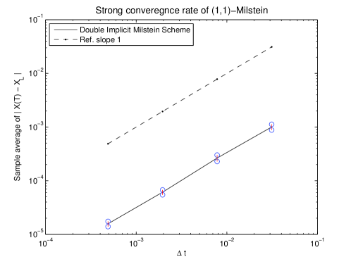
Figure 2: Strong error of double-implicit Milstein scheme applied to Heston 3/2 Stochastic volatility model.

Although we do not know the explicit form of the solution, Theorem 4.8 guarantees that the (1,1)-Milstein scheme (2.14) strongly converges to the true solution. We therefore take the (1,1)-Milstein scheme with $\Delta t=2^{-14}$ as a reference solution. We compare this with the (1,1)-Milstein scheme evaluated with $(2\Delta t,2^{3}\Delta t,2^{5}\Delta t,2^{7}\Delta t)$ in order to estimate the rate of convergence. Since we are using a Monte Carlo method, the sampling error decays like $1/\sqrt{M}$, where $M=10000$ is the number of sample paths. From Figure 2 we see that there appears to exist a positive constant $C$ such that

$$e^{\mathrm{strong}}_{\Delta t}\leq C\Delta t,\quad\hbox{for sufficiently small $\Delta t$}.$$

A least squares fit for equality produced the value $1.1304$ for the rate with residual of $0.2468$. Hence, our results are consistent with strong order of convergence equal to one.

5 Conclusions

Our aim was to introduce a new discretization scheme that can be shown to work well on highly nonlinear SDEs arising in mathematical finance and to possess excellent linear and nonlinear stability properties. There are several interesting areas for follow-up work; most notably (a) establishing a strong order of convergence for this method in a nonlinear setting, and (b) developing a theory of positivity preservation in the case of SDE systems and their numerical simulation.

References

- [1] D.H. Ahn and B. Gao. A parametric nonlinear model of term structure dynamics. Review of Financial Studies, 12(4):721, 1999.
- [2] Y. Ait-Sahalia. Testing continuous-time models of the spot interest rate. Review of Financial Studies, 9(2):385–426, 1996.
- [3] J. A. D. Appleby, M. Guzowska, C. Kelly, and A. Rodkina. Preserving positivity in solutions of discretised stochastic differential equations. Applied Mathematics and Computation, 217(2):763–774, 2010.
- [4] T.C. Gard. Introduction to Stochastic Differential Equations. Marcel Dekker, New York, 1988.
- [5] M. Giles. Improved multilevel Monte Carlo convergence using the Milstein scheme. Monte Carlo and Quasi-Monte Carlo Methods 2006, pages 343–358, 2006.
- [6] M.B. Giles. Multilevel Monte Carlo path simulation. Operations Research-Baltimore, 56(3):607–617, 2008.
- [7] J. Goard and M. Mazur. Stochastic volatility models and the pricing of vix options. Mathematical Finance, 2011.
- [8] I. Gyöngy. A note on Euler’s approximations. Potential Analysis, 8(3):205–216, 1998.
- [9] S.L. Heston. A simple new formula for options with stochastic volatility. Course notes of Washington University in St. Louis, Missouri, 1997.
- [10] D.J. Higham. A-stability and stochastic mean-square stability. BIT Numerical Mathematics, 40(2):404–409, 2000.
- [11] D.J. Higham. Mean-square and asymptotic stability of the stochastic theta method. SIAM Journal on Numerical Analysis, 38:753–769, 2001.
- [12] M. Hutzenthaler, A. Jentzen, and P.E. Kloeden. Strong and weak divergence in finite time of Euler’s method for stochastic differential equations with non-globally Lipschitz continuous coefficients. Proceedings of the Royal Society A, 467(2130):1563–1576, 2011.
- [13] A. Jentzen, P.E. Kloeden, and A. Neuenkirch. Pathwise approximation of stochastic differential equations on domains: higher order convergence rates without global Lipschitz coefficients. Numerische Mathematik, 112(1):41–64, 2009.
- [14] C. Kahl, M. Gunther, and T. Rosberg. Structure preserving stochastic integration schemes in interest rate derivative modeling. Applied Numerical Mathematics, 58(3):284–295, 2008.
- [15] C. Kahl and H. Schurz. Balanced Milstein methods for ordinary SDEs. Monte Carlo Methods and Applications, 12(2):143–170, 2006.
- [16] I. Karatzas and S.E. Shreve. Brownian Motion and Stochastic Calculus. Springer, 1991.
- [17] P.E. Kloeden and E. Platen. Numerical Solution of Stochastic Differential Equations. Springer, 1992.
- [18] A.L. Lewis. Option Valuation Under Stochastic Volatility. Finance Press, 2000.
- [19] R.S. Liptser and A.N. Shiryayev. Theory of Martingales. Kluwer Academic Publishers, 1989.
- [20] R. Lord, R. Koekkoek, and D.J.C. Van Dijk. A comparison of biased simulation schemes for stochastic volatility models. Quantitative Finance, 10(2):177–194, 2009.
- [21] G.N. Milstein, E. Platen, and H. Schurz. Balanced implicit methods for stiff stochastic systems. SIAM Journal on Numerical Analysis, 35(3):1010–1019, 1998.
- [22] G.N. Milstein and M.V. Tretyakov. Stochastic Numerics for Mathematical Physics. Scientific Computation. Springer-Verlag, Berlin, 2004.
- [23] H. Schurz. Convergence and stability of balanced implicit methods for systems of SDEs. Int. J. Numer. Anal. Model, 2(2):197–220, 2005.
- [24] Y. Shen, Q. Luo, and X. Mao. The improved LaSalle-type theorems for stochastic functional differential equations. Journal of Mathematical Analysis and Applications, 318(1):134–154, 2006.
- [25] A.N. Shiryaev. Probability. Springer-Verlag, New York, 1996.
- [26] L. Szpruch. Strong convergence of stochastic dissipative systems with super-linear diffusion term. Stochastics, 2012, to appear.
- [27] L. Szpruch and X. Mao. Strong convergence of numerical methods for nonlinear stochastic differential equations under monotone conditions. working paper, 2010.
- [28] L. Szpruch, X. Mao, D.J. Higham, and J. Pan. Numerical simulation of a strongly nonlinear Ait-Sahalia type interest rate model. BIT Numerical Mathematics, 51:405–425, 2011.
- [29] E. Zeidler. Nonlinear Functional Analysis and its Applications. Springer Verlag, 1985.