How Correlations Influence Lasso Prediction

Abstract

We study how correlations in the design matrix influence Lasso prediction. First, we argue that the higher the correlations are, the smaller the optimal tuning parameter is. This implies in particular that the standard tuning parameters, that do not depend on the design matrix, are not favorable. Furthermore, we argue that Lasso prediction works well for any degree of correlations if suitable tuning parameters are chosen. We study these two subjects theoretically as well as with simulations.
Keywords: Correlations, Lars Algorithm, Lasso, Restricted Eigenvalue, Tuning Parameter.

1 Introduction

Although the Lasso estimator is very popular and correlations are present in many of its diverse applications, the influence of these correlations is still not entirely understood. Correlations are surely problematic for parameter estimation and variable selection. The influence of correlations on prediction, however, is far less clear.

Let us first set the framework for our study. We consider the linear regression model

$$Y=X\beta_{0}+\sigma\epsilon,$$ (1)

where $Y\in\mathbb{R}^{n}$ is the response vector, $X\in\mathbb{R}^{n\times p}$ is the design matrix, $\epsilon\in\mathbb{R}^{n}$ is the noise and $\sigma\in\mathbb{R}^{+}$ is the noise level. We assume in the following that the noise level $\sigma$ is known and that the noise $\epsilon$ obeys an $n$ dimensional normal distribution with covariance matrix equal to the identity. Moreover, we assume that the design matrix $X$ is normalized, that is, $\left(X^{T}X\right)_{jj}=n$ for $1\leq j\leq p$. Three main tasks are then usually considered: estimating $\beta_{0}$ (parameter estimation), selecting the non-zero components of $\beta_{0}$ (variable selection), and estimating $X\beta_{0}$ (prediction). Many applications of the above regression model are high dimensional, that is, the number of variables $p$ is larger than the number of observations $n$ but are also sparse, that is, the true solution $\beta_{0}$ has only few nonzero entries. A computationally feasible method for the mentioned tasks is, for instance, the widely used Lasso estimator introduced in [Tib96]:

$$\hat{\beta}:=\operatorname*{arg\,min}_{\beta\in\mathbb{R}^{p}}\left\{\|Y-X\beta\|_{2}^{2}+\lambda\|\beta\|_{1}\right\}.$$

In this paper, we focus on the prediction error of this estimator for different degrees of correlations. The literature on the Lasso estimator has become very large, we refer the reader to the well written books [BC11, BvdG11, HTF01] and the references therein.

Two types of bounds for the prediction error are known in the theory for the Lasso estimator. On the one hand, there are the so called fast rate bounds (see [BRT09, BTW07b, vdGB09] and references therein). These bounds are nearly optimal but imply restricted eigenvalues or similar conditions and therefore only apply for weakly correlated designs. On the other hand, there are the so called slow rate bounds (see [HCB08, KTL11, MM11, RT11]). These bounds are valid for any degree of correlations but - as their name suggests - are usually thought of as unfavorable.

Regarding the mentioned bounds, one could claim that correlations lead in general to large prediction errors. However, recent results in [vdGL12] suggest that this is not true. It is argued in [vdGL12] that for (very) highly correlated designs, small tuning parameters can be chosen and favorable slow rate bounds are obtained. In the present paper, we provide more insight into the relation between Lasso prediction and correlations. We find that the larger the correlations are, the smaller the optimal tuning parameter is. Moreover, we find both in theory and simulations that Lasso performs well for any degree of correlations if the tuning parameter is chosen suitably.

We finally give a short outline of this paper: we first discuss the known bounds on the Lasso prediction error. Then, after some illustrating numerical results, we study the subject theoretically. We then present several simulations, interpret our results and finally close with a discussion.

2 Known Bounds for Lasso Prediction

To set the context of our contribution, we first discuss briefly the known bounds for the prediction error of the Lasso estimator. We refer to the books [BC11] and [BvdG11] for a detailed introduction to the theory of the Lasso.

Fast rate bounds, on the one hand, are bounds proportional to the square of the tuning parameter $\lambda$. These bounds are only valid for weakly correlated design matrices. We first recall the corresponding assumption. Let $a$ be a vector in $\mathbb{R}^{p}$, $J$ a subset of $\{1,\ldots,p\}$, and finally $a_{J}$ the vector in $\mathbb{R}^{p}$ that has the same coordinates as $a$ on $J$ and zero coordinates on the complement $J^{c}$. Denote the cardinality of a given set by $|\cdot|$. For a given integer $\bar{s}$, the Restricted Eigenvalues (RE) assumption introduced in [BRT09] reads then

Assumption RE($\bar{s}$):

$$\phi(\bar{s}):=\min_{J_{0}\subset\{1,\ldots,p\}:|J_{0}|\leq\bar{s}}\min_{\Delta\neq 0:\|\Delta_{J_{0}^{c}}\|_{1}\leq 3\|\Delta_{J_{0}}\|_{1}}\frac{\|X\Delta\|_{2}}{\sqrt{n}\|\Delta_{J_{0}}\|_{2}}>0.$$

The integer $\bar{s}$ plays the role of a sparsity index and is usually comparable to the number of nonzero entries of $\beta_{0}$. More precisely, to obtain the following fast rates, it is assumed that $\bar{s}\geq s$, where $s:=|\{j:(\beta_{0})_{j}\neq 0\}|$. Also, we notice that $\phi(\bar{s})\approx 0$ corresponds to correlations. Under the above assumption it holds (see for example Bickel et al. [BRT09] and more recently Koltchinskii et al. [KTL11]):

$$\|X(\hat{\beta}-\beta_{0})\|_{2}^{2}\leq\frac{\lambda^{2}\bar{s}}{n\phi^{2}(\bar{s})}$$ (2)

on the set $\mathcal{T}:=\left\{\sup_{\beta}\frac{2\sigma|\epsilon^{T}X\beta|}{\|\beta\|_{1}}\leq\lambda\right\}$. Similar bounds, under slightly different assumptions, can be found in [vdGB09]. Usually, the tuning parameter $\lambda$ is chosen proportional to $\sigma\sqrt{n\log(p)}$. For fixed $\phi$, the above rate then is optimal up to a logarithmic term (see [BTW07a, Theorem 5.1]) and the set $\mathcal{T}$ has a high probability (see Section 3.2.2). For correlated designs, however, this choice of the tuning parameter is not suitable. This is detailed in the following section.

Slow rate bounds, on the other hand, are bounds only proportional to the tuning parameter $\lambda$. These bounds are valid for arbitrary designs, in particular, they are valid for highly correlated designs. The result [KTL11, Eq. (2.3) in Theorem 1] yields in our setting

$$\|X(\hat{\beta}-\beta_{0})\|_{2}^{2}\leq 2\lambda\|\beta_{0}\|_{1}$$ (3)

on the set $\mathcal{T}$. Similar bounds can be found in [HCB08] (for a related work on a truncated version of the Lasso), in [MM11, Theorem 3.1] (for estimation of a general function in a Banach space), and in [RT11, Theorem 4.1] (which also applies to the non-parametric setting; note that the corresponding bound can be written in the form above with arbitrary tuning parameter $\lambda$). We note that these bounds depend on $\|\beta_{0}\|_{1}$ instead of $\bar{s}$. Moreover, they depend on $\lambda$ to the first power, and these bounds are therefore considered unfavorable compared to the fast rate bounds.

The mentioned bounds are only useful for sufficiently large tuning parameters such that the set $\mathcal{T}$ has a high probability. This is crucial for the following. We show that the higher the correlations, the larger the probability of $\mathcal{T}$ is. Correlations thus allow for small tuning parameters; this implies for correlated designs, via the factor $\lambda$ in the slow rate bounds, favorable bounds even though no fast rate bounds are available.

Remark 2.1.

The slow rate bound (3) can be improved if $\|\beta_{0}\|_{1}$ is large. Indeed, we proof in the Appendix that

$$\|X(\hat{\beta}-\beta_{0})\|_{2}^{2}\leq 2\lambda\min\left\{\|\beta_{0}\|_{1}\ ,\ \|(\hat{\beta}-\beta_{0})_{J_{0}}\|_{1}\right\}$$

on the set $\mathcal{T}$. That is, the prediction error can be bounded both with $\|\beta_{0}\|_{1}$ and with the $\ell_{1}$ estimation error restricted on the sparsity pattern of $\beta_{0}$. The latter term can be considerably smaller than $\|\beta_{0}\|_{1}$ (in particular for weakly correlated designs). A detailed analysis of this observation, however, is not within the scope of the present paper.

3 The Lasso and Correlations

We show in this section that correlations strongly influence the optimal tuning parameters. Moreover, we show that - for suitably chosen tuning parameters - Lasso performs well in prediction for different levels of correlations. For this, we first present simulations where we compare Lasso prediction for an initial design with Lasso prediction for an expanded design with additional impertinent variables. Then, we discuss the theoretical aspects of correlations. We introduce, in particular, a simple and illustrating notion about correlations. Further simulations finally confirm our analysis.

3.1 The Lasso on Expanded Design Matrices

Is Lasso prediction becoming worse when many impertinent variables are added to the design? Regarding the bounds and the usual value of the tuning parameter $\lambda$ described in the last section, one may expect that many additional variables lead to notably larger optimal tuning parameters and prediction errors. However, as we see in the following, this is not true in general.

Let us first describe the experiments.

Algorithm 1

We simulate from the linear regression model (1) and take as input the number of observations $n$, the number of variables $p$, the noise level $\sigma$, the number of nonzero entries of the true solution $s:=\left\{j:(\beta_{0})_{j}\neq 0\right\}$ and finally a correlation factor $\rho\in[0,1)$. We then sample the $n$ independent rows of the design matrix $X$ from a normal distribution with mean zero and covariance matrix with diagonal entries equal to $1$ and off-diagonal entries equal to $\rho$, and we normalize $X$ such that $(X^{\top}X)_{jj}=n$ for $1\leq j\leq n$. Then, we define $(\beta_{0})_{i}:=1$ for $1\leq i\leq s$ and $(\beta_{0})_{i}:=0$ otherwise, sample the error $\epsilon$ from a standard normal distribution and compute the response vector $Y$ according to (1). After calculating the Lasso solution $\hat{\beta}$, we finally compute the prediction error $\|X(\hat{\beta}-\beta_{0})\|_{2}^{2}$ for different tuning parameters $\lambda$ and find the optimal tuning parameter, that is, the tuning parameter that leads to the smallest prediction error.

Algorithm 2

This algorithm only differs from the above algorithm in one point. In an additional step after the initial design matrix $X$ is sampled, we add for each column $X^{(j)}$ of the initial design matrix $p\text{~{}-~{}}1$ columns sampled according to $X^{(j)}+\eta N$. We finally normalize the resulting matrix. The parameter $\eta$ controls the correlation among the added columns and the initial columns and $N$ is a standard normally distributed random vector. Compared to the initial design, we have now a design with $p^{2}\text{~{}-~{}}p$ additional impertinent variables.

Several algorithms for computing a Lasso solution have been proposed: For example, using interior point methods [CDS98], using homotopy parameters [EHJT04, OPT00, Tur05], or using a so-called shooting algorithm [DDDM04, Fu98, FHHT07]. We use the LARS algorithm introduced in [EHJT04], since, among others, Bach et al. [BJMO11, Section 1.7.1] have confirmed the good behavior of this algorithm when the variables are correlated.

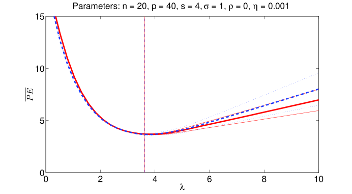
Figure 1: We plot the mean values $\overline{PE}$ of the prediction errors $\|A\hat{\beta}-A\beta_{0}\|_{2}^{2}$ for $1000$ iterations as a function of the tuning parameter $\lambda$. The blue, dashed line corresponds to Algorithm 1, where $A$ stands for the initial design matrices. The blue, dotted lines give the confidence bounds. The red, solid line corresponds to Algorithm 2, where $A$ represents the extended matrices. The faint, red lines give the confidence bounds. The parameters for the algorithms are given in the header. The mean of the optimal tuning parameters is $3.62\pm 0.01$ for Algorithm 1 and $3.63\pm 0.01$ for Algorithm 2. These values are represented by the blue and red vertical lines.

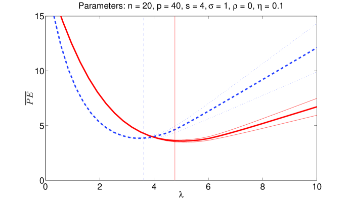
Figure 2: We plot the mean values $\overline{PE}$ of the prediction errors $\|A\hat{\beta}-A\beta_{0}\|_{2}^{2}$ for $1000$ iterations as a function of the tuning parameter $\lambda$. The blue, dashed line corresponds to Algorithm 1, where A stands for the initial design matrices. The blue, dotted lines give the confidence bounds. The red, solid line corresponds to Algorithm 2, where A stands for the extended matrices. The faint, red lines give the confidence bounds. The parameters for the algorithms are given in the header. The mean of the optimal tuning parameters is $3.63\pm 0.01$ for Algorithm 1 and $4.77\pm 0.01$ for Algorithm 2. These values are represented by the blue and red vertical lines.

Results

We did $1000$ iterations of the above algorithms for different $\lambda$ and with $n=20$, $p=40$, $s=4$, $\sigma=1$, $\rho=0$ and with $\eta=0.001$ (Figure 1) and $\eta=0.1$ (Figure 2). We plot the means $\overline{PE}$ of the prediction errors as a function of $\lambda$. The blue, dashed curves correspond to the initial designs (Algorithm 1), the red, solid curves correspond to the extended designs (Algorithm 2). The confidence bounds are plotted with faint lines in the according color and finally the mean values of the optimal tuning parameters are plotted with vertical lines.
We find in both examples that the minimal prediction errors, that is, the minima of the red and blue curves, do not differ significantly. Additionally, in the first example, corresponding to highly correlated added variables ($\eta=0.001$, see Figure 1), also the optimal tuning parameters do not differ significantly. However, in the second example ($\eta=0.1$, see Figure 2), the optimal tuning parameter is considerably larger for the extended designs.

First Conclusions

Our results indicate that tuning parameters proportional to $\sqrt{n\log p}$ (cf. [BRT09] and most other contributions on the subject) independent of the degree of correlations are not favorable. Indeed, for Algorithm 2, this would lead to a tuning parameter proportional to $\sqrt{n\log p^{2}}=\sqrt{2n\log p}$, whereas for Algorithm 1 to $\sqrt{n\log p}$. But regarding Figure 1, the two optimal tuning parameters are nearly equal and hence these choices are not favorable. In contrast, the results illustrate that the optimal tuning parameters depend strongly on the level of correlations: for Algorithm 2 (red, solid curves), the means of the optimal tuning parameters corresponding to the highly correlated case ($3.63\pm 0.01$, see Figure 1) are be considerably smaller than the ones corresponding to the weakly correlated case ($4.77\pm 0.01$, see Figure 2).
Our results indicate additionally that the minimal mean prediction errors are comparable for all cases. This implies, that a suitable tuning parameters lead to good prediction even with additional impertinent parameters. We only give two examples here but made these observations for any values of $n$, $p$ and $s$.

3.2 Theoretical Evidence

We provide in this section theoretical explanations for the above observations. For this, we first discuss results derived in [vdGL12]. They find that high correlations allow for small tuning parameters and that this can lead to bounds for Lasso prediction that are even more favorable than the fast rate bounds. Then, we introduce and apply new correlation measures that provide some insight for (in contrast to [vdGL12]) arbitrary degrees of correlations. For no correlations, in particular, these results simplify to the classical results.

3.2.1 Highly Correlated Designs

First results for the highly correlated case are derived in [vdGL12]. Crucial in their study is the treatment of the stochastic term with metric entropy.

The bound on the prediction error for Lasso reads as follows:

Lemma 3.1.

[vdGL12, Theorem 4.1 & Corollary 4.2] On the set

$$\mathcal{T}_{\alpha}:=\left\{\sup_{\beta}\frac{2\sigma|\epsilon^{T}X\beta|}{\|X\beta\|_{2}^{1-\alpha}\|\beta\|_{1}^{\alpha}}\leq\widetilde{\lambda}\right\}$$

we have for $\lambda=(2\widetilde{\lambda}n^{\alpha-1})^{\frac{2}{1+\alpha}}\|\beta_{0}\|_{1}^{\frac{\alpha-1}{1+\alpha}}$ and $0<\alpha<1$

$$\|X(\hat{\beta}-\beta_{0})\|_{2}^{2}\leq\frac{21}{2}\left(2\widetilde{\lambda}n^{\alpha-1}\right)^{\frac{2}{1+\alpha}}\|\beta_{0}\|_{1}^{\frac{2\alpha}{1+\alpha}}.$$

We show in the following that for high correlations the stochastic term $\mathcal{T}_{\alpha}$ has a high probability even for small $\alpha$ and thus favorable bounds are obtained. The parameter $\alpha$ can be thought of as a measure of correlations: $\alpha$ small corresponds to high correlations, $\alpha$ large corresponds to small correlations.

The stochastic term $\mathcal{T}_{\alpha}$ is estimated using metric entropy. We recall, that the covering numbers $N(\delta,\mathcal{F},d)$ measure the complexity of a set $\mathcal{F}$ with respect to a metric $d$ and a radius $\delta$. Precisely, $N(\delta,\mathcal{F},d)$ is the minimal number of balls of radius $\delta$ with respect to the metric $d$ needed to cover $\mathcal{F}$. The entropy numbers are then defined as $H(\delta,\mathcal{F},d):=\log N(\delta,\mathcal{F},d)$. In this framework, we say that the design is highly correlated if the covering numbers $N(\delta,\operatorname{sconv}\{X^{(1)},...,X^{(p)}\},\|\cdot\|_{2})$ (or the corresponding entropy numbers) increase only mildly with $1/\delta$, where $\{X^{(1)},...,X^{(p)}\}$ are the columns of the design matrix and $\operatorname{sconv}$ denotes the symmetric convex hull. This is specified in the following lemma:

Lemma 3.2.

[vdGL12, Corollary 5.2] Let $0<\alpha<1$ be fixed. Then, assuming

$$\log\left(1+N(\sqrt{n}\delta,\operatorname{sconv}\{X^{(1)},...,X^{(p)}\},\|\cdot\|_{2})\right)\leq\left(\frac{A}{\delta}\right)^{2\alpha},0<\delta\leq 1,$$ (4)

there exists a value $C(\alpha,A)$ depending on $\alpha$ and $A$ only such that for all $\kappa>0$ and for

$$\widetilde{\lambda}=\sigma C(\alpha,A)\sqrt{n^{2-\alpha}\log(2/\kappa)},$$

the following bound is valid:

$$\mathbb{P}(\mathcal{T}_{\alpha})\geq 1-\kappa.$$

We observe indeed that the smaller $\alpha$ is, the higher the correlations are. We also mention that Assumption (4) only applies to highly correlated designs. An example is given in [vdGL12]: the assumption is met if the eigenvalues of the Gram matrix $\frac{X^{T}X}{n}$ decrease sufficiently fast.

Lemma 3.1 and Lemma 3.2 can now be combined to the following bound for the prediction error of the Lasso:

Theorem 3.1.

With the choice of $\lambda$ as in Lemma 3.1 and under the assumptions of Lemma 3.2, it holds that

$$\|X(\hat{\beta}-\beta_{0})\|_{2}^{2}\leq\frac{21}{2}\left(\sigma C(\alpha,A)\sqrt{n^{\alpha}\log(2/\kappa)}\right)^{\frac{2}{1+\alpha}}\|\beta_{0}\|_{1}^{\frac{2\alpha}{1+\alpha}}$$

with probability at least $1-\kappa$.

High correlations allow for small values of $\alpha$ and lead therefore to favorable bounds. For $\alpha$ sufficiently small, these bounds may even outmatch the classical fast rate bounds. For moderate or weak correlations, however, Assumption (4) is not met and therefore the above lemma does not apply.

3.2.2 Arbitrary Designs

In this section, we introduce bounds that apply to any degree of correlations. The correlations are in particular allowed to be moderate or small and the bounds simplify to the classical results for weakly correlated designs. We first introduce two measure for correlations that are then used to bound the stochastic term. These results are then combined with the classical slow rate bound to obtain a new bound for Lasso prediction. We finally give some simple examples.

Two Measures for Correlations

We introduce two numbers that measure the correlations in the design. For this, we first define the correlation function $K:\mathbb{R}^{+}_{0}\to\mathbb{N}$ as

$$K(x):=\min\{ l\in\mathbb{N}:\exists x^{(1)},\ldots,x^{(l)}\in\sqrt{n}S^{n-1},$$ (5)

$$X^{(m)}\in(1+x)\operatorname{sconv}\{x^{(1)},\ldots,x^{(l)}\}~{}\forall 1\leq m\leq p\},$$

where $S^{n-1}$ denotes the unit sphere in $\mathbb{R}^{n}$. We observe that $K(x)\leq p$ for all $x\in\mathbb{R}_{0}^{+}$ and that $K$ is a decreasing function of $x$. A measure for correlations should, as the metric entropy above, measure how close to one another the columns of the design matrix are. Indeed, for moderate $x$, $K(x)\approx p$ for uncorrelated designs, whereas $K(x)$ may be considerably smaller for correlated designs. This information is concentrated in the correlation factors that we define as

$$K_{\kappa}:=\inf_{x\in\mathbb{R}_{0}^{+}}(1+x)\sqrt{\frac{\log(2K(x)/\kappa)}{\log(2p/\kappa)}},$$

$\kappa\in(0,1]$, and as

$$F:=\inf_{x\in\mathbb{R}_{0}^{+}}(1+x)\sqrt{\frac{\log(1+K(x))}{\log(1+p)}}.$$

Since $K(0)\leq p$, it holds that $F,K_{\kappa}\in(0,1]$. We also note that similar quantities could can be defined for $p=\infty$ (removing the normalization). In any case, large $F$ and $K_{\kappa}$ correspond to uncorrelated designs, whereas small $F$ and $K_{\kappa}$ correspond to correlated designs.

Control of the Stochastic Term

We now show that small correlation factors allow for small tuning parameters and thus lead to favorable bounds for Lasso prediction. Crucial in our analysis is again the treatment of a stochastic term similar to the one above.

We prove the following bound in the appendix:

Theorem 3.2.

With the definitions above, $\mathcal{T}$ as defined in Section 2 and for all $\kappa>0$ and $\lambda\geq\lambda_{\kappa}:=K_{\kappa}2\sigma\sqrt{2n\log(2p/\kappa)}$, it holds that

$$\mathbb{P}\left(\mathcal{T}\right)\geq 1-\kappa.$$

Additionally, independently of the choice of $\lambda$,

$$\mathbb{E}\left[\sup_{\|\beta\|_{1}\leq M}\sigma\mid\epsilon^{T}X\beta\mid\right]\leq F\sigma\sqrt{\frac{8n\log(1+p)}{3}}M.$$

For small correlation factors $K_{\kappa}$ and $F$, the minimal tuning parameters $\lambda_{\kappa}$ and the expectation of the stochastic term are small. For $K_{\kappa}\to 1$, the minimal tuning parameters simplify to $2\sigma\sqrt{2n\log(2p/\kappa)}$ (cf. [BRT09]). Similarly, for $F\to 1$, the expectation of the stochastic term simplifies to $\sigma\sqrt{\frac{8n\log(1+p)}{3}}M$.

Together with the slow rate bound introduced in Section 2, this permits the following bound:

Corollary 3.1.

For $\lambda\geq\lambda_{\kappa}$ it holds that

$$\|X(\hat{\beta}-\beta_{0})\|_{2}^{2}\leq 2\lambda\|\beta_{0}\|_{1}$$

with probability at least $1-\kappa$.

Our contribution to this result concerns the tuning parameters: for the classical value $\lambda=2\sigma\sqrt{2n\log(2p/\kappa)}$, the bound simplifies to the classical slow rate bounds. Correlations, however, allow for smaller $\lambda$ and thus lead to more favorable bounds.

Let us have a look at some general aspects of the above bound. Most importantly, Corollary 3.1 applies to any degree of correlations. In contrast, Theorem 3.1 only applies for highly correlated designs, and the classical fast rate bounds only apply for weakly correlated designs. We also observe that the sparsity index $\bar{s}$, which appears in the classical fast rate bounds, does not appear in Corollary 3.1. Hence, Corollary 3.1 can be useful even if the true regression vector $\beta_{0}$ is only approximately sparse. However, for very large $\|\beta_{0}\|_{1}$, the bound is unfavorable. An example in this context can be found in [CP09, Section 2.2]. (However, we do not agree with their conclusions corresponding to this example. We stress, in contrast, that correlation are not problematic in general.) We finally refer to Remark 2.1 and to [MM11] for some additional considerations on the optimality of this kind of bounds.

Remark 3.1 (Weakly Correlated Designs).

Corollary 3.1 holds for any degree of correlations because it follows directly from the classical slow rate bound and the properties of the refined tuning parameter. However, for weakly correlated designs, we can also make use of the refined tuning parameter to improve the classical fast rate bound by a factor $K_{\kappa}^{2}$. Usually, the gain is moderate, but in special cases such as sparse designs (see Example 3.2), the gain can be large. Finally, we note that optimal rates, that is, lower bounds for the prediction error $\|X(\hat{\beta}-\beta_{0})\|_{2}^{2}$, are available for weakly correlated designs. The optimal rate is then $s\log(1+\frac{p}{s})$ and is deduced from Fano’s Lemma (see [BTW07a, Theorem 5.1, Lemma A.1]). For similar results in matrix regression, we refer to [KTL11], where the assumptions on the design needed for such lower bounds are explicitly stated (see, in particular, their Assumption 2).

Examples

In this final section, we illustrate some properties of the correlation numbers $K_{\kappa}$ and $F$ for various settings. We consider, in particular, design matrices with different geometric properties and with different degrees of correlations.

$\hookrightarrow$ Example 3.1 (Low Dimensional Design).

Let $\operatorname{dim}~{}\operatorname{span}\{X^{(1)},...,X^{(p)}\}\leq W$. Then,

$$X^{(j)}\in\sqrt{W}~{}\operatorname{sconv}\{x_{1},...,x_{W}\}~{}\text{for all}~{}1\leq j\leq p$$

for properly chosen $x_{1},...,x_{W}\in\sqrt{n}S^{n-1}$ (for example orthogonal vectors in a suitable subspace). Hence, $K_{\kappa}\leq(1+\sqrt{W})\sqrt{\frac{\log(2W/\kappa)}{\log(2p/\kappa)}}$ and $F\leq(1+\sqrt{W})\sqrt{\frac{\log(1+W)}{\log(1+p)}}$.

$\hookrightarrow$ Example 3.2 (Sparse Design).

Let the number of non-zero coefficients in $X^{(j)}$ be such that $\|X^{(j)}\|_{0}\leq d$ for all $1\leq j\leq p$, with $d\leq n$. Then,

$$X^{(j)}\in\sqrt{d}\operatorname{sconv}\{x_{1},...,x_{n}\}~{}\text{for all}~{}1\leq j\leq p$$

for properly chosen $x_{1},...,x_{n}\in\sqrt{n}S^{n-1}$ (for example orthogonal vectors in $\mathbb{R}^{n}$). Hence, $K_{\kappa}\leq\sqrt{d}\sqrt{\frac{\log(2n/\kappa)}{\log(2p/\kappa)}}$ and $F\leq\sqrt{d}\sqrt{\frac{\log(1+n)}{\log(1+p)}}$.

$\hookrightarrow$ Example 3.3 (Weakly Correlated Design).

We consider a weakly correlated design with $p\gg n$. It turns out that the results in Section 3.2.1 lead to a tuning parameter $\lambda\sim n$ . This implies in particular that the results in Section  3.2.1, unlike the results in this section, do not simplify to the classical results for uncorrelated designs. We give a sketch of the proof in the Appendix.

$\hookrightarrow$ Example 3.4 (Highly Correlated Design).

We illustrate with an example that highly correlated designs indeed involve small correlation factors $K_{\kappa}$. This implies, in accordance to the simulation results, that tuning parameters depending on the design rather than tuning parameters depending only on $\sigma$, $n$, and $p$ should be applied.
Let us describe how the design matrix $X$ is chosen: Fix an arbitrary $n$ dimensional vector $X^{(1)}$ of Euclidian norm $\sqrt{n}$. Then, we add $p-1$ columns sampled according to $X^{(1)}+\nu N$ where $\nu$ is a positive (but small) constant and $N$ is a standard normally distributed random vector. We finally normalize the resulting matrix.
For simplicity, we do not give explicit constants but present a coarse asymptotic result that highlights the main ideas. For this, we consider the number of variables $p$ as a function of the number of observations $n$ and impose the usual restrictions in high dimensional regression, that is, $p\sim n^{w}$ for a $w\in\mathbb{N}$. If the correlations are sufficiently large, more precisely $\nu\leq\frac{1}{\sqrt{8}n}$, it holds that

$$K_{\kappa}\to\frac{1}{\sqrt{w}}\ \text{~{}as~{}}n\to\infty$$

with probability tending to 1. This implies especially that the standard tuning parameters $\sim\sigma\sqrt{n\log p}$ can be considerably too large if $\nu$ is large. The proof of the above statement is given in the Appendix.

$\hookrightarrow$ Example 3.5 (Equal Columns).

Let the cardinality of the set $|\{X^{(j)}:1\leq j\leq p\}|=v$. Then, $K_{\kappa}\leq\sqrt{\frac{\log(2v/\kappa)}{\log(2p/\kappa)}}$ and $F\leq\sqrt{\frac{\log(1+v)}{\log(1+p)}}$.

3.3 Experimental Study

We consider Algorithm 1 with different sets of parameters to make statements about the influence of the single parameters on Lasso prediction. In particular, we are interested in the influence of the correlations $\rho$.

Table 1: The means of the optimal tuning parameters $\overline{\lambda}_{min}$ and the means of the minimal prediction errors $\overline{PE}_{min}$ calculated according to Algorithm 1 with 1000 iterations and for different sets of parameters.

$n$	$p$	$s$	$\sigma$	$\rho$	$\overline{\lambda}_{min}$	$\overline{PE}_{min}$
$20$	$40$	$4$	$1$	$0.99$	$0.69\pm 0.03$	$1.77\pm 0.05$
				$0.9$	$1.58\pm 0.03$	$2.37\pm 0.04$
				$0$	$3.60\pm 0.03$	$3.17\pm 0.03$
$50$	$40$	$4$	$1$	$0.99$	$0.67\pm 0.03$	$1.29\pm 0.04$
				$0.9$	$1.71\pm 0.03$	$1.85\pm 0.03$
				$0$	$3.91\pm 0.03$	$3.48\pm 0.02$
$20$	$400$	$4$	$1$	$0.99$	$0.97\pm 0.03$	$1.75\pm 0.05$
				$0.9$	$2.11\pm 0.04$	$2.58\pm 0.04$
				$0$	$4.82\pm 0.03$	$3.34\pm 0.03$
$20$	$40$	$10$	$1$	$0.99$	$0.59\pm 0.03$	$6.50\pm 0.22$
				$0.9$	$1.46\pm 0.03$	$7.97\pm 0.19$
				$0$	$2.90\pm 0.03$	$6.65\pm 0.06$
$20$	$40$	$4$	$3$	$0.99$	$2.42\pm 0.15$	$6.16\pm 0.17$
				$0.9$	$5.33\pm 0.13$	$6.47\pm 0.14$
				$0$	$12.33\pm 0.10$	$3.80\pm 0.03$

Results

We collect in Table 1 the means of the optimal tuning parameters $\overline{\lambda}_{min}$ and the means of the minimal prediction errors $\overline{PE}_{min}$ for 1000 iterations and different parameter sets. Let us first highlight the two most important observations: first, correlations ($\rho$ large) lead to small tuning parameters. Second, correlations do not necessarily lead to high prediction errors. In contrast, the prediction errors are mostly smaller for the correlated settings.
Let us now make some other observations. First, we find that the optimal tuning parameters do not increase considerably when the number of observations $n$ is increased. In contrast, the means of the minimal prediction errors decrease for the correlated case as expected, whereas this is not true for the uncorrelated case.
Second, increasing the number of variables $p$ leads to increasing optimal tuning parameters as expected (interestingly by factors close to $\sqrt{\frac{\log 400}{\log 40}}$, cf. Corrollary 3.1). The means of the minimal prediction errors do, surprisingly, not increase considerably.
Third, as expected, increasing the sparsity $s$ does not considerably influence the optimal tuning parameters but leads to increasing means of the minimal prediction errors.
Forth, for $\sigma=3$ both the optimal tuning parameter as well as the mean of the minimal prediction error increase approximately by a factor $3$. The mean of the minimal prediction errors for $\sigma=3$ and $\rho=0$ is an exception and remains unclear.
We finally mention that we obtained analogeous results for many other values of $\beta_{0}$ and sets of parameters.

Conclusions

The experiments illustrate the good performance of the Lasso estimator for prediction even for highly correlated designs. Crucial is the choice of the tuning parameters: we found that the optimal tuning parameters depend highly on the design. This implies in particular that choosing $\lambda$ proportional to $\sqrt{n\log{p}}$ independent of the design is not favorable.

4 Discussion

Our study suggests that correlations in the design matrix are not problematic for Lasso prediction. However, the tuning parameter has to be chosen suitable to the correlations. Both, the theoretical results and the simulations strongly indicate that the larger the correlations are, the smaller the optimal tuning parameter is. This implies in particular, that the tuning parameter should not be chosen only as a function of the number of observations, the number of parameters and the variance. The precise dependence of the optimal tuning parameter on the correlations is not known, but we expect that cross validation provides a suitable choice in many applications.

Acknowledgments

We thank Sara van de Geer for the great support. Moreover, we thank Arnak Dalalyan, who read a draft of this paper carefully and gave valuable and insightful comments. Finally, we thank the reviewers for their helpful suggestions and comments.

Appendix

Proof of Remark 2.1.

By the definition of the Lasso estimator, we have

$$\|Y-X\hat{\beta}\|_{2}^{2}+\lambda\|\hat{\beta}\|_{1}\leq\|Y-X\beta_{0}\|_{2}^{2}+\lambda\|\beta_{0}\|_{1}.$$

This implies, since $Y=X\beta_{0}+\sigma\epsilon$, that

$$\|X(\hat{\beta}-\beta_{0})\|_{2}^{2}\leq 2\sigma|\epsilon^{T}X(\hat{\beta}-\beta_{0})|+\lambda\|\beta_{0}\|_{1}-\lambda\|\hat{\beta}\|_{1}.$$

Next, on the set $\mathcal{T}$, we have $2\sigma|\epsilon^{T}X(\hat{\beta}-\beta_{0})|\leq\lambda\|\hat{\beta}-\beta_{0}\|_{1}$. Additionally, by the definition of $J_{0}$,

$$\|\hat{\beta}-\beta_{0}\|_{1}=\|(\hat{\beta}-\beta_{0})_{J_{0}}\|_{1}+\|\hat{\beta}_{J_{0}^{c}}\|_{1}.$$

Combining these two arguments and using the triangular inequality, we get

$$\|X(\hat{\beta}-\beta_{0})\|_{2}^{2} \leq \lambda\|(\hat{\beta}-\beta_{0})_{J_{0}}\|_{1}+\lambda\|\hat{\beta}_{J_{0}^{c}}\|_{1}+\lambda\|\beta_{0}\|_{1}-\lambda\|\hat{\beta}\|_{1}$$

$$\leq 2\lambda\|(\hat{\beta}-\beta_{0})_{J_{0}}\|_{1}.$$

On the other hand, using the triangular inequality, we also get

$$\|X(\hat{\beta}-\beta_{0})\|_{2}^{2}\leq\lambda\|\hat{\beta}-\beta_{0}\|_{1}+\lambda\|\beta_{0}\|_{1}-\lambda\|\hat{\beta}\|_{1}\leq 2\lambda\|\beta_{0}\|_{1}.$$

This completes the proof.

∎

Proof of Theorem 3.2.

We first show that for a fixed $x\in\mathbb{R}^{+}_{0}$, the parameter space $\{\beta\in\mathbb{R}^{p}:\|\beta\|_{1}\leq M\}$ can be replaced by the $K(x)$ dimensional parameter space $\{\beta\in\mathbb{R}^{K(x)}:\|\beta\|_{1}\leq(1+x)M\}$. Then, we bound the stochastic term in expectation and probability and eventually take the infimum over $x\in\mathbb{R}^{+}_{0}$ to derive the desired inequalities.
As a start, we assume without loss of generality $\sigma=1$, we fix $x\in\mathbb{R}_{0}^{+}$ and set $K:=K(x)$. Then, according to the definition of the correlation function (5), there exist vectors $x^{(1)},...,x^{(K)}\in\sqrt{n}S^{n-1}$ and numbers $\{\kappa_{j}(m):1\leq j\leq K\}$ for all $1\leq m\leq p$ such that $X^{(m)}=\sum_{j=1}^{K}\kappa_{j}(m)x^{(j)}$ and $\sum_{j=1}^{K}|\kappa_{j}(m)|\leq(1+x)$. Thus,

$$(X\beta)_{i}=\sum_{m=1}^{p}X^{(m)}_{i}\beta_{m}=\sum_{m=1}^{p}\sum_{j=1}^{K}\kappa_{j}(m)x^{(j)}_{i}\beta_{m}=\sum_{j=1}^{K}x^{(j)}_{i}\sum_{m=1}^{p}\kappa_{j}(m)\beta_{m}$$

and additionally

$$\sum_{j=1}^{K}|\sum_{m=1}^{p}\kappa_{j}(m)\beta_{m}|\leq\sum_{m=1}^{p}|\beta_{m}|\sum_{j=1}^{K}|\kappa_{j}(m)|\leq(1+x)\|\beta\|_{1}.$$

These two results imply

$$\sup_{\|\beta\|_{1}\leq M}\mid\epsilon^{T}X\beta\mid\leq\sup_{\|\widetilde{\beta}\|_{1}\leq(1+x)M}\mid\epsilon^{T}\widetilde{X}\widetilde{\beta}\mid,$$

where $\widetilde{\beta}\in\mathbb{R}^{K}$ and $\widetilde{X}:=(x^{(1)},...,x^{(K)})$. That is, we can replace the $p$ dimensional parameter space by a $K$ dimensional parameter space at the price of an additional factor $1+x$.
We now bound the stochastic term in expectation. First, we obtain by Cauchy-Schwarz’s Inequality

$$\mathbb{E}\left[\sup_{\|\widetilde{\beta}\|_{1}\leq(1+x)M}\mid\epsilon^{T}\widetilde{X}\widetilde{\beta}\mid\right] =\mathbb{E}\left[\sup_{\|\widetilde{\beta}\|_{1}\leq(1+x)M}|\sum_{i=1}^{n}\sum_{j=1}^{K}\epsilon_{i}\widetilde{X}^{(j)}_{i}\widetilde{\beta}_{j}|\right]$$

$$\leq\left[\mathbb{E}\sup_{\|\widetilde{\beta}\|_{1}\leq(1+x)M}\|\widetilde{\beta}\|_{1}\max_{1\leq j\leq K}\mid\epsilon^{T}\widetilde{X}^{(j)}\mid\right]$$

$$=(1+x)M\mathbb{E}\left[\max_{1\leq j\leq K}\mid\epsilon^{T}\widetilde{X}^{(j)}\mid\right].$$

Next (cf. the proof of [vdGL11, Lemma 3]), we obtain for $\Psi(x):=e^{x^{2}}-1$

$$\mathbb{E}\left[\max_{1\leq j\leq K}\mid\epsilon^{T}\widetilde{X}^{(j)}\mid\right]\leq\Psi^{-1}(K)\max_{1\leq j\leq K}\|\epsilon^{T}\widetilde{X}^{(j)}\|_{\Psi},$$

where $\|\cdot\|_{\Psi}$ denotes the Orlicz norm with respect to the function $\Psi$ (see [vdGL11] for a definition). Since $\frac{\epsilon^{T}\widetilde{X}^{(j)}}{\sqrt{n}}$ is standard normally distributed, we obtain $\|\frac{\epsilon^{T}\widetilde{X}^{(j)}}{\sqrt{n}}\|_{\Psi}=\sqrt{\frac{8}{3}}$ (see for example [vdVW00, Page 100]). Moreover, one may check that $\Psi^{-1}(y)=\sqrt{\log(1+y)}$. Consequently,

$$\mathbb{E}\left[\sup_{\|\widetilde{\beta}\|_{1}\leq(1+x)M}\mid\epsilon^{T}\widetilde{X}\widetilde{\beta}\mid\right] \leq(1+x)M\sqrt{\frac{8n\log(1+K)}{3}}$$

One can then derive the second assertion of the theorem by taking the infimum over $x\in\mathbb{R}_{0}^{+}$.
As a next step, we deduce similarly as above (compare also to [BRT09])

$$\mathbb{P}\left(\sup_{\|\beta\|_{1}\leq M}2\mid\epsilon^{T}X\beta\mid\geq\lambda M\right)\leq \mathbb{P}\left(\sup_{\|\widetilde{\beta}\|_{1}\leq 1}2\mid\epsilon^{T}\widetilde{X}\widetilde{\beta}\mid\geq\frac{\lambda}{1+x}\right)$$

$$\leq K\max_{1\leq j\leq K}\mathbb{P}\left(\left|\epsilon^{T}\frac{\widetilde{X}^{(j)}}{\sqrt{n}}\right|\geq\frac{\lambda}{2(1+x)\sqrt{n}}\right)$$

$$= K\mathbb{P}\left(|\gamma|\geq\frac{\lambda}{2(1+x)\sqrt{n}}\right),$$

where $\gamma$ is a standard normally distributed random variable. Setting $\lambda:=2(1+x)\sqrt{2n\log(2K/\kappa)}$, we obtain

$$\mathbb{P}\left(\sup_{\|\beta\|_{1}\leq M}2\mid\epsilon^{T}X\beta\mid\geq\lambda M\right) \leq 2K\exp{\left(\text{-}\frac{\lambda^{2}}{8(1+x)^{2}n}\right)}$$

$$=2K\exp{\left(\text{-}\log(2K/\kappa)\right)}$$

$$=\kappa.$$

The first assertion can finally be derived taking the infimum over $x\in\mathbb{R}_{0}^{+}$ and applying monotonous convergence. ∎

Proposition 1.

It holds for all $0<\delta\leq 1$

$$\left(\frac{1}{\delta}\right)^{n}\leq N(\delta,\{x\in\mathbb{R}^{n}:\|x\|_{2}\leq 1\},\|\cdot\|_{2})\leq\left(\frac{3}{\delta}\right)^{n}.$$

Proof.

If a collection of balls covers the set $\{x\in\mathbb{R}^{n}:\|x\|_{2}\leq 1\}$, the volume covered by these balls is at least as large as the volume of $\{x\in\mathbb{R}^{n}:\|x\|_{2}\leq 1\}$. Thus,

$$N(\delta,\{x\in\mathbb{R}^{n}:\|x\|_{2}\leq 1\},\|\cdot\|_{2})\cdot\delta^{n}\geq 1,$$

and the left inequality follows. The right inequality can be deduced similarly. ∎

Proof Sketch for Example 3.3.

For weakly correlated designs and for $p$ very large, it holds that

$$\log\left(1+N(\sqrt{n}\delta,\operatorname{sconv}\{X^{(1)},...,X^{(p)}\},\|\cdot\|_{2})\right)$$

$$\approx \log\left(N(\delta,\{x\in\mathbb{R}^{n}:\|x\|_{2}\leq 1\},\|\cdot\|_{2})\right).$$

We can then apply Proposition 1 to deduce

$$\log\left(1+N(\sqrt{n}\delta,\operatorname{sconv}\{X^{(1)},...,X^{(p)}\},\|\cdot\|_{2})\right)\approx n\log(1/\delta).$$

Hence, Lemma 3.2 requires that $A$ fulfills for all $0<\delta\leq 1$ (in fact, it is sufficient for $\frac{1}{\sqrt{n}}\lesssim\delta\leq 1$, see the proofs in [Led10] for this refinement)

$$\left(\frac{A}{\delta}\right)^{2\alpha}\approx n\log(1/\delta)$$

and thus

$$A^{\alpha}\approx\delta^{\alpha}\sqrt{n\log(1/\delta)}.$$

We can maximize the right hand side over $0<\delta\leq 1$ and plug the result into [vdGL12, Corollary 5.2] to deduce the result. ∎

Proof for Example 3.4.

The realizations of the random vectors $X^{(1)}+\nu N$ are clustered with high probability and can thus be described (in the sense of the definition of $K_{\kappa}$) by much less than $p$ vectors.
To see this, consider $X^{(1)}$ and a rotation $R\in\operatorname{SO(n)}$ such that $RX^{(1)}=(\sqrt{n},0,\dots,0)^{T}$. Moreover, let $N$ be a standard normally distributed random vector in $\mathbb{R}^{n}$, $n\geq 2$. The measure corresponding to the random vector $N$ is denoted by $\mathbb{P}$. We then obtain with the triangle inequality and the condition on $\nu$

$$\mathbb{P}\left(\left|1-\frac{\sqrt{n}}{\|RX^{(1)}+\nu RN\|_{2}}\right|\geq{1}\right)= \mathbb{P}\left(\frac{\|RX^{(1)}+\nu RN\|_{2}}{\sqrt{n}}\leq\frac{1}{2}\right)$$

$$\leq \mathbb{P}\left(\frac{\|X^{(1)}\|_{2}-\nu\|N\|_{2}}{\sqrt{n}}\leq\frac{1}{2}\right)$$

$$= \mathbb{P}\left(\frac{\nu\|N\|_{2}}{\sqrt{n}}\geq\frac{1}{2}\right)$$

$$\leq \mathbb{P}\left(\|N\|_{2}\geq\frac{\sqrt{n}}{2\nu}\right)$$

$$\leq \mathbb{P}\left(\|N\|_{2}\geq\sqrt{2n}\right).$$

Now, we can bound the $l_{1}$ distance of the vector $\frac{\sqrt{n}(RX^{(1)}+\nu RN)}{\|RX^{(1)}+\nu RN\|_{2}}$ generated according to our setting to the vector $RX^{(1)}$:

$$\mathbb{P}\left(\left\|RX^{(1)}-\frac{\sqrt{n}(RX^{(1)}+\nu RN)}{\|RX^{(1)}+\nu RN\|_{2}}\right\|_{1}\geq 2{\sqrt{n}}\right)$$

$$\leq \mathbb{P}\left(\left|1-\frac{\sqrt{n}}{\|RX^{(1)}+\nu RN\|_{2}}\right|\|RX^{(1)}\|_{1}\geq{\sqrt{n}}\right)+\mathbb{P}\left(\|{\nu RN}\|_{1}\geq{\|RX^{(1)}+\nu RN\|_{2}}\right)$$

$$\leq \mathbb{P}\left(\left|1-\frac{\sqrt{n}}{\|RX^{(1)}+\nu RN\|_{2}}\right|\geq 1\right)+\mathbb{P}\left(\sqrt{n}\nu\|N\|_{2}\geq\sqrt{n}-{\nu\|N\|_{2}}\right)$$

$$\leq \mathbb{P}\left(\|N\|_{2}\geq\sqrt{2n}\right)+\mathbb{P}\left(\|N\|_{2}\geq\frac{1}{2\nu}\right)$$

$$\leq 2\mathbb{P}\left(\|N\|_{2}\geq\sqrt{2n}\right).$$

It can be derived easily from standard results (see for example [BvdG11, Page 254]) that

$$\mathbb{P}\left(\|N\|_{2}\geq\sqrt{2n}\right)\leq\exp\left(\text{-}\frac{n}{8}\right).$$

Consequently,

$$\mathbb{P}\left(\left\|RX^{(1)}-\frac{\sqrt{n}(RX^{(1)}+\nu RN)}{\|RX^{(1)}+\nu RN\|_{2}}\right\|_{1}\geq 2\sqrt{n}\right)\leq 2\exp\left(\text{-}\frac{n}{8}\right).$$ (6)

Finally, define for any $0\leq z\leq 2\sqrt{n}$ the set

$$\mathcal{C}_{z}:=\{(\sqrt{n},z,0,\dots,0)^{T} ,(\sqrt{n},\text{-}z,0,\dots,0)^{T},(\sqrt{n},0,z,0,\dots,0)^{T},$$

$$\hskip 71.13188pt(\sqrt{n},0,\text{-}z,0,\dots,0)^{T},\dots\}\subset\mathbb{R}^{n}$$

These vectors will play the role of the vectors $x^{(1)},...,x^{(l)}$ in Definition (5). It holds that

$$\operatorname{card}(\mathcal{C}_{z})=2(n-1)$$ (7)

and

$$\mathcal{C}_{z}\subset\sqrt{n+z^{2}}~{}S^{n-1}.$$ (8)

Moreover,

$$\{x\in\mathbb{R}^{n}:\|x-RX^{(1)}\|_{1}\leq z\}\cap\sqrt{n}S^{n-1}\subset\operatorname{sconv}(\mathcal{C}_{z}).$$ (9)

Inequality (6) and Inclusion (9) imply that with probability at least $1-2\exp\left(\text{-}\frac{n}{8}\right)$

$$\frac{\sqrt{n}(X^{(1)}+\nu N)}{\|RX^{(1)}+\nu RN\|_{2}}\in\operatorname{sconv}(R^{T}\mathcal{C}_{{2\sqrt{n}}}).$$

Thus, using Equality (7) and Inclusion (8), we have $K(\sqrt{5}-1)\leq 2(n-1)$ with probability at least $1-2(p-1)\exp\left(\text{-}\frac{n}{8}\right)$. ∎