Investigation of frustrated and dimerized classical Heisenberg chains

Abstract

We have considered the 1D dimerized frustrated antiferromagnetic (ferromagnetic) Heisenberg model with arbitrary spin $S$. The exact classical magnetic phase diagram at zero temperature is determined using the LK cluster method. Cluster method results, show that the classical ground state phase diagram of the model is very rich including first and second-order phase transitions. In the absence of the dimerization, a second-order phase transition occurs between antiferromagnetic (ferromagnetic) and spiral phases at the critical frustration $\alpha_{c}=\pm 0.25$. In the vicinity of the critical points $\alpha_{c}$, the exact classical critical exponent of the spiral order parameter is found $1/2$. In the case of dimerized chain ($\delta\neq 0$), the spiral order shows stability and exists in some part of the ground state phase diagram. We have found two first-order critical lines in the ground state phase diagram. These critical lines separate the antiferromagnetic from spiral phase.

I Introduction

During the last decades several classical techniques such as the well-known Luttinger-Tisza methodLuttinger46 , vertex modelBaxter and so on have been introduced to solve classical Hamiltonian exactly. The Luttinger-Tisza method is more effective in systems with bilinear interactions and vertex model usually applied for treating frustrated modelLieb ; Sutherland .

In a very recent workTK2009 , T. Kaplan have used a kind of cluster method, hereafter simply LK method, which is based on a block of three spins to solve frustrated classical Heisenberg model in one dimension with added nearest neighbor biquadratic exchange interactions. He asserted that the LK method is not limited to one dimension or to translationally invariant spin HamiltoniansLyons64 and expanded his approach to determine the phase diagram of frustrated classical Heisenberg and XY models with added nearest neighbor biquadratic exchange interactions in $d=2$ dimensionLX2010 . In order to check the validity of Kaplan’s phase diagram conjecture, we have investigated his modelTK2009 form quantum point of view for spin-$\frac{1}{2}$ with an accurate algorithm (Lanczos method), and our results, which will be presented elsewhereJaSaee , showed that LK method, albeit is a classical approach but has the capability to work for aspects of a quantum treatment.

Actually, these are our stimulating reasons to take a quite well known frustrated and dimerized Heisenberg model and determine its classical ground state phase diagram exactly with strong, but not well known LK method which is able to solve problems rigorouslyTK2009 . Let us start with definition of the dimerized and frustrated Heisenberg model as follow

$$\emph{H}=J_{1}\sum_{n}\Big{[}1+(-1)^{n}\delta\Big{]}\textbf{S}_{n}\cdot\textbf{S}_{n+1}+J_{2}\sum_{n}\textbf{S}_{n}\cdot\textbf{S}_{n+2},$$ (1)

where $\vec{S}_{n}$ is the $n$th classical vector of the length $S$. A spin system is frustrated when the global order because of the competition of different kinds of interaction is incompatible with the local order, so chain with both antiferromagnetic-antiferromagnetic exchanges $(J_{1}>0,J_{2}>0)$ and ferromagnetic-antiferromagnetic exchanges $(J_{1}<0,J_{2}>0)$, hereafter simply AF-AF and F-AF respectively, are frustrated.

Quantum study of this model is well done for the spin-1/2 and spin-1 chainsShastry81 ; Bouzerar98 ; Nakamura97 ; Kumar07 ; Chitra95 ; Controzzi05 ; Pati96 ; Oshikawa . It is found that the quantum fluctuations play a very important role at zero temperature in the ground state phase diagram of the models. This model shows a dimerization transition at $\delta=\delta_{c}$.

For system with spin half, $S=1/2$, $\delta_{c}=0$ is the transition point, which is related to the Lieb-Schultz-Mattis theorem (states that system should be in either twofold degeneracy or gapless excitations of the ground states at $\delta=0$). Indeed, for AF-AF case and on the undimerized link $\delta=0$, there is a critical frustration parameter $\alpha_{c}=0.2411$Haldane82 ; Okamoto92 . The dimerization transition at $\delta=\delta_{c}=0$ is of second order and system for $\alpha<\alpha_{c}$ shows a gapless Tomonaga-Luttinger Liquid (TLL). But, for $\alpha>\alpha_{c}$, the ground state is doubly degenerate, showing a spontaneous dimerization. This is a signature of a first-order dimerization transition at $\delta=\delta_{c}=0$.

On the other hand, system with spin one, $S=1$, with $\delta=0$ and small $\alpha=\frac{J_{2}}{J_{1}}$ lives in Haldane phase and does not represent a transition line. In contrast, dimerization transition between the Haldane phase and the dimerized phase happensAffleck87 ; Kolezhuk96 at a finite $\delta_{c}$, which depends on the $\alpha$ (know as frustration parameter). As matter of fact, for system with spin one, there is a critical frustration $\alpha_{c}$ point which is second order form of transition. This critical point separates a TLL phase for $\alpha<\alpha_{c}$ from first order one for $\alpha>\alpha_{c}$.

But there is not a classical clear picture of different ground state phases of the mentioned model. Having a classical picture, from one hand help us to know that quantum fluctuations destroy which one of the classical orderings. On the other hand for arbitrary large spin model, the classical picture is the same with the quantum picture of the ground state phase diagram. In this work we focus on the 1D frustrated and dimerized systems with arbitrary spin $S$ (see FIG. 1). To find the exact classical ground state phase diagram of the model, the LK cluster method is used. In the absence of the dimerization, by increasing the frustration a classical phase transition occurs at $\alpha_{c}=+0.25~{}(-0.25)$ from the antiferromagnetic (ferromagnetic) phase into the spiral magnetic phase. Our results show that the dimerization parameter induces new magnetic phases including stripe-antiferromagnetic phase (or uud and duu phases). Existing of these magnetic phases is independent of length of spins.

The outline of the paper is as follows. In forthcoming section we will extensively explain the LK method with implementing it to our model and in the section III we will summarize our results.

II the LK cluster method

In order to implement LK method we follow exactly the procedure in Ref. [2]. Without losing the generality and setting periodic boundary conditions, Eq.(1) can be rewritten as:

$$\emph{H}_{c}=\sum_{i}h_{c}\big{(}\textbf{S}_{i-1},\textbf{S}_{i},\textbf{S}_{i+1}\big{)},$$ (2)

where the ”cluster energy” involve three neighboring spins is

$$h_{c}(\textbf{S}_{1},\textbf{S}_{2},\textbf{S}_{3}) = \frac{J_{1}}{2}\Big{\{}\big{(}1-\delta\big{)}\textbf{S}_{1}\cdot\textbf{S}_{2}+\big{(}1+\delta\big{)}\textbf{S}_{2}\cdot\textbf{S}_{3})\Big{\}}$$ (3)

$$+ J_{2}(\textbf{S}_{1}\cdot\textbf{S}_{3}).$$

It is clear that

$$\emph{H}_{c}\geq\sum_{j}min~{}h_{c}(\overrightarrow{S}_{j-1},\overrightarrow{S}_{j},\overrightarrow{S}_{j+1}).$$ (4)

To minimize $h_{c}$ respect spins directions, we first consider coplanar spins, and label the angles $\theta$, $\theta^{\prime}$ made by the end spins with the central spin (see FIG. 2) which in coplanar case we set $\phi=0,\phi^{\prime}=0$. The cluster energy is given by

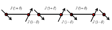
Figure 1: (Color online.) The schematic picture of dimerized spins chain.

$$h_{c}(\theta,\theta^{\prime}) = S^{2}\Big{\{}\big{(}\frac{1-\delta}{2}\big{)}\cos\theta+\big{(}\frac{1+\delta}{2}\big{)}\cos\theta^{\prime}$$ (5)

$$+ \alpha\cos(\theta-\theta^{\prime})\Big{\}},$$

where $\alpha=J_{2}/J_{1}$. Minimizing $h_{c}$ respect $\theta$, $\theta^{\prime}$ gives the following equation:

$$\frac{\partial h_{c}}{\partial\theta}=-\frac{S^{2}}{2}\Big{[}(1-\delta)\sin\theta+2\alpha\sin(\theta-\theta^{\prime})\Big{]}$$

$$\frac{\partial h_{c}}{\partial\theta^{\prime}}=-\frac{S^{2}}{2}\Big{[}(1+\delta)\sin\theta^{\prime}-2\alpha\sin(\theta-\theta^{\prime})\Big{]}.$$ (6)

Let’s first deal with a case without dimerization, by setting $\delta=0$ in Eq. (6) we have

$$\frac{\partial h_{c}}{\partial\theta}=-\frac{S^{2}}{2}\Big{[}\sin\theta+2\alpha\sin(\theta-\theta^{\prime})\Big{]}$$

$$\frac{\partial h_{c}}{\partial\theta^{\prime}}=-\frac{S^{2}}{2}\Big{[}\sin\theta^{\prime}-2\alpha\sin(\theta-\theta^{\prime})\Big{]}.$$ (7)

its solutions are

$$(\theta,\theta^{\prime}) = (0,0),(\pi,\pi),(\pi,0),(0,\pi),$$

$$(\theta,\theta^{\prime}) = (\theta_{0},-\theta_{0}),~{}~{}~{}\text{(Spiral- type)},~{}~{}~{}\text{where}$$

$$\cos\theta_{0} = -\frac{1}{4\alpha}\rightarrow|\alpha|\geq\frac{1}{4}.$$

The solutions $(\pi,\pi),(0,0)$ are related to collinear antiferromagnetic and ferromagnetic states respectively. The antiferromagnetic (ferromagnetic) state will minimize the energy in the case of $J_{1}>0$ ($J_{1}<0$). Solutions $(\pi,0)\rightarrow(\downarrow,\uparrow,\uparrow)$ and $(0,\pi)\rightarrow(\uparrow,\uparrow,\downarrow)$ are degenerate states and show spins propagate in the down-up-up and up-up-down respectively Lyons64 . Spiral state $(\theta_{0},-\theta_{0})$ with uniform rotation is also degenerate state. In following we present results of the antiferromagnetic case $J>0$.

By setting minimization conditions into the Eq. (5) we have the following energies:

$$h_{\text{antiferro}} = h_{c}(\pi,\pi)=S^{2}(-1+\alpha),$$

$$h_{\text{uudd}} = h_{c}(0,\pi)=S^{2}(-\alpha),$$

$$h_{\text{spiral}} = h_{c}(\theta_{0},-\theta_{0})=S^{2}(-\frac{1}{8\alpha}-\alpha).$$ (9)

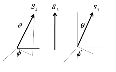
Figure 2: Spins cluster configuration.

By equating these energies in pairs we have found only one critical point, $\alpha_{c}=0.25$. Because of the continuity in the derivative $\frac{\partial h_{c}}{\partial\alpha}$, a second-order phase transition occurs when passing trough $\alpha=0.25$. The ground state is in the antiferromagnetic phase in the region of the frustration $\alpha<0.25$ and in the spiral phase in region $\alpha>0.25$. In general, the antiferromagnetic phase is recognized by the non-zero value of the Neel order parameter defined as

$$M_{st}^{z}=\frac{1}{N}\sum_{n}(-1)^{n}S_{n}^{z},$$ (10)

and the spiral phase in the ground state phase diagram of the spin systems is characterized by the nonzero value of the spiral order parameter

$$\chi=\frac{1}{N}\sum_{n}|{\bf S}_{n}\times{\bf S}_{n+1}|.$$ (11)

Using Eq. (LABEL:e7) we have found the spiral order parameter as

$$\chi = 0~{}~{}~{}~{}~{}~{}~{}~{}~{}~{}~{}~{}~{}~{}~{}~{}~{}~{},~{}~{}~{}\alpha<\alpha_{c},$$

$$\chi = S^{2}\sqrt{1-\frac{\alpha_{c}^{2}}{\alpha^{2}}}~{}~{}~{}~{},~{}~{}~{}\alpha>\alpha_{c}.$$ (12)

In FIG.3, we have plotted the spiral order parameter as a function of the frustration parameter $\alpha$ for the non-dimerized model ($\delta=0$). As is clearly seen from this figure, there is no long-range spiral order in the region of frustration $\alpha<\alpha_{c}=0.25$. However, in the region $\alpha>\alpha_{c}=0.25$ the spins of the system show a profound spiral order which grows by increasing the frustration parameter $\alpha$.

It has been discovered that continuous phase transitions have many interesting properties. The phenomena associated with continuous phase transitions are called critical phenomena, due to their association with critical points. It turns out that continuous phase transitions can be characterized by parameters known as critical exponents. Critical exponents describe the behavior of physical quantities near continuous phase transitions. It is believed, that they are universal, i.e. they do not depend on the details of the physical system. Our analytical results show that the spiral order parameter $\chi$ approaches zero in a singular fashion as $\alpha$ approaches $\alpha_{c}$, vanishing asymptotically as

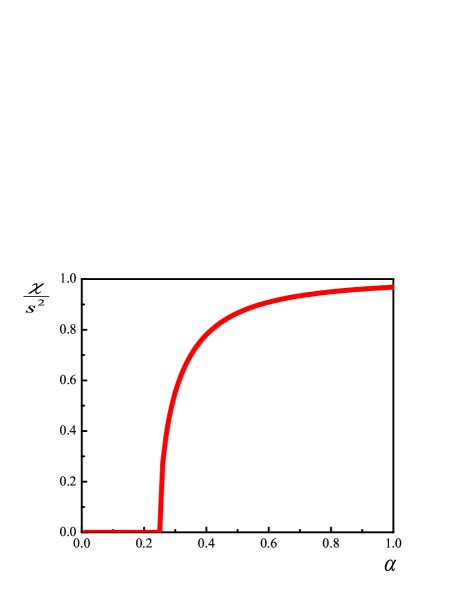
Figure 3: (Color online). The spiral order parameter as a function of the frustration parameter $\alpha$ in the case of non-dimerized chain ($\delta=0$).

$$\chi\propto(1-\frac{\alpha_{c}}{\alpha})^{1/2},$$ (13)

which shows that the critical exponent for spiral order parameter is a simple fraction $\varepsilon=1/2$.

Now, we back to our original problem $\delta\neq 0$, finding the exact ground state phase diagram of the classical frustrated and dimerized Heisenberg chains. One can immediately see the possibility of having two spirals, one on the even sites, the other on the odd sites, both with the same wave length, but with a phase difference as described in the following:

To use the cluster approach for the case of non-zero dimerization, $\delta\neq 0$, one must consider two types of cluster, one being $(\bullet\quad\bullet\bullet)$, the other being $(\bullet\bullet\quad\bullet)$. Let us label the spins in the first cluster $(S_{1}\quad S_{2}S_{3})$, and the second $(S_{2}\quad S_{3}S_{4})$ and continue $(S_{3}\quad S_{4}S_{5})$ , $(S_{4}\quad S_{5}S_{6})$, $\cdots$. The 2-spiral form assumes a simple spiral on the even sites, and a simple spiral on odd sites, both with the same turn angle between spins, which we called $2\theta_{0}$. Calling the angles $-\theta_{0}+\epsilon$ and $\theta_{0}+\epsilon$, respectively, of $S_{1}$ and $S_{3}$ with the center spin $S_{2}$ in the first cluster, then gives $2\theta_{0}$ as the angle between $S_{1}$ and $S_{3}$. Then, preserving the angle between $S_{2}$ and $S_{3}$ in the next cluster, (which is now $-\theta_{0}-\epsilon$ , since the central spin is now $S_{3}$) and the angle between $S_{3}$ and $S_{4}$ being taken as$\theta_{0}-\epsilon$ gives the angle $2\theta_{0}$ between $S_{2}$ and $S_{4}$. Hence the first two clusters begin to show the spiral on the odd sites and the spiral on the even sites. Continuing this to the next few clusters shows that this allows a description of a system with two spirals, one on the odd, the other on the even sites, both with the same turn-angle $2\theta_{0}$ or wavelength. Also the energy of each cluster is the same, so one can consider just one cluster, say the first one above, in figuring out the relation between $\epsilon$ and $\delta$. For the case of $2\theta_{0}=\pi/2$, spins order as following pattern $(\nwarrow\uparrow\nearrow\longrightarrow\searrow\downarrow\swarrow\longleftarrow\nwarrow)$. Therefor, in the case ($\delta\neq 0$), the following solutions can satisfy the minimum energy condition,

$$(\theta,\theta^{\prime}) = (0,0),(\pi,\pi),(\pi,0),(0,\pi),$$

$$(\theta,\theta^{\prime}) = (\theta_{0},-\theta_{0}+\epsilon),~{}~{}~{}\text{(Spiral- type)},~{}~{}~{}\text{where}$$

$$\cos\theta_{0} = -\frac{16\delta\alpha^{2}-(1-\delta)^{2}}{4\alpha(1-\delta)^{2}(1+\delta)}.$$

$$\sin\theta_{0} = 0\rightarrow\theta_{0}=n\pi\rightarrow\epsilon=0.$$

By substituting them into the Eq.(5), the ground state energy of cluster in different sectors becomes

$$h_{\text{antiferro}} = h_{c}(\pi,\pi)=S^{2}(-1+\alpha),$$

$$h_{\text{uud}} = h_{c}(0,\pi)=S^{2}(-\delta-\alpha),$$

$$h_{\text{duu}} = h_{c}(\pi,0)=S^{2}(\delta-\alpha),$$

$$h_{\text{spiral}} = h_{c}(\theta_{0},-\theta_{0}+\epsilon)=S^{2}\Big{(}\frac{\delta-1}{2}$$

$$+ (1+\cos\theta_{0})\big{\{}(1-\delta)+\sqrt{(1-\delta)^{2}\cos^{2}\theta_{0}+4\delta}\big{\}}\Big{)}.$$

As it can be seen from the above equations, in respect to the case of $\delta=0$, dimerization exchange removed the degeneracy between $(\downarrow,\uparrow,\uparrow)$ and $(\uparrow,\uparrow,\downarrow)$ states. The $(\downarrow,\uparrow,\uparrow)$ state, defines as a phase with opposite magnetization on odd ($J(1-\delta)$) bonds, but $(\uparrow,\uparrow,\downarrow)$ state denotes by opposite magnetization on even ($J(1+\delta)$) bonds. Using the conditions in Eq. (LABEL:e9) allow us to find the stability of different phases. Doing some calculations, one can find two critical lines as

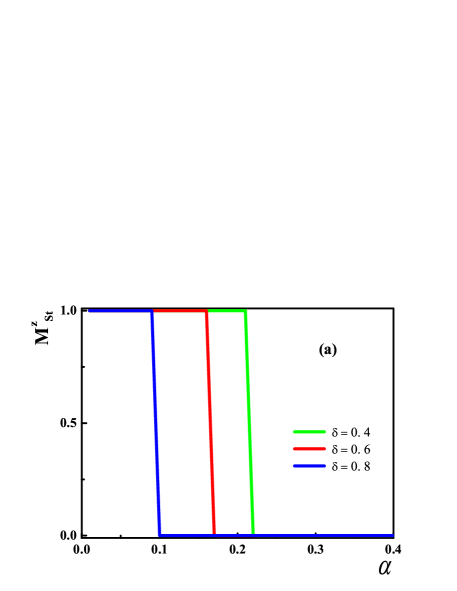
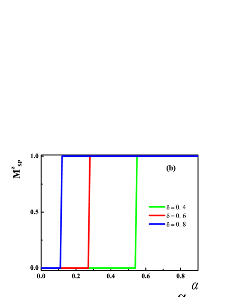
Figure 4: (Color online). The staggered magnetization $M_{st}$ and stripe-antiferromagnetic $M_{sp}$ order parameters as function of the frustration $\alpha$ for different values of the frustration $\delta=0.4,0.6,0.8$.

$$\alpha_{\tilde{c}} = \frac{1-\delta^{2}}{4\delta},$$

$$\alpha_{\tilde{c}} = \frac{\delta^{2}-1}{4\delta}.$$ (15)

These critical lines separate spiral phase from the uud and the duu phases. There is a discontinuity in the derivative $\frac{\partial h_{c}}{\partial\delta}$, and therefore a first-order phase transition through the mentioned critical lines. In addition, one should note that the ordering of the uud and duu phases, in principle is a type of the stripe-antiferromagnetic phaseMahdavifar08 ; Mahdavifar10 . Therefore, the order parameter for distinguishing these phases is defined as

$$M_{sp}^{z} = \frac{2}{N}\sum_{n=1}(-1)^{n+1}(S_{2n-1}^{z}+S_{2n}^{z}),~{}for~{}uud$$ (16)

$$= \frac{2}{N}\sum_{n=1}(-1)^{n+1}(S_{2n}^{z}+S_{2n+1}^{z}),~{}for~{}duu.$$

We have also found antiferromagnetic phase that is stable for

$$\alpha < \frac{1-\delta^{2}}{4}~{}for~{}\delta>0,$$

$$\alpha > \frac{\delta^{2}-1}{4}~{}for~{}\delta<0.$$ (17)

It is completely clear that in uud and duu phases, $M_{sp}^{z}$ takes the value $1$. In FIG. 4 (a), we have plotted $M_{st}^{z}$ as a function of the frustration $\alpha$ for different values of the frustration $\delta=0.4,0.6,0.8$. As it can seen from this figure, for $\alpha<\alpha_{c}$, the staggered magnetization is equal to $1.0$, which shows that the ground state of the system is in the fully polarized antiferromagnetic phase. Finally, it is clear that there is no antiferromagnetic ordering in the region $\alpha>\alpha_{c}$. In FIG. 4 (b), we have the same picture for the stripe antiferromagnetic order function. The zero value of $M_{sp}^{z}$ in the region $\alpha<\alpha_{\tilde{c}}$ is in complete agreement with the fully polarized antiferromagnetic and spiral phases in this region. By more increasing the dimerization and for $\alpha>\alpha_{\tilde{c}}$, clearly be seen that the ground state of the system is in the uud. Also one predicts that the tripe antiferromagnetic as a function of the $\alpha$ displays a jump for certain parameters which is one of the most important indications of the first-order phase transition. We emphasize that a first-order phase transition occurs between the spiral and the duu phases, for negative values of the dimerization.

The FIG. (5) shows the exact classical ground state phase diagram of the model in $\delta-\alpha$ plane. It should be mentioned that the same phase diagram can be also found in the ferromagnetic side which we do not depict. In the absence of dimerization, $\delta=0$, there are antiferromagnetic(ferromagnetic) and spiral phases which is separated by two critical point at $\alpha_{c}=\pm 0.25$ which the negative sign refers to ferromagnetic side. The second order phase transition occurs at these critical points. By turning dimerization the spiral phase persists to be stable in $\frac{1-\delta^{2}}{4}<\alpha<\frac{1-\delta^{2}}{4\delta}$ region for $\delta>0$ and $\frac{\delta^{2}-1}{4\delta}{4}<\alpha<\frac{1-\delta^{2}}{4}$ region for $\delta<0$. The antiferromagnetic phase remains stable up to the critical line $\frac{1-\delta^{2}}{4}$. The uud and duu phases propagate with different energy and separated by two first order critical lines, ($\frac{1-\delta^{2}}{4\delta}$ and $\frac{\delta^{2}-1}{4\delta}$), from spiral phase.

In the following we are interested to implement LK method to non-coplanar antiferromagnetic case. Again with using cluster approach and without losing generality, labeled the angles $(\theta,\phi)$ ,$(\theta^{\prime},\phi^{\prime})$ made by the end spins with the central spin (see FIG. 2). Then the cluster energy is determine as

$$h_{c}(\theta,\theta^{\prime}) = S^{2}\Big{\{}\Big{(}\frac{1-\delta}{2}\Big{)}\cos\theta+\Big{(}\frac{1+\delta}{2}\Big{)}\cos\theta^{\prime}$$

$$+ \alpha\Big{[}\cos\theta\cos\theta^{\prime}+\sin\theta\sin\theta^{\prime}\cos(\phi-\phi^{\prime})\Big{]}\Big{\}}.$$

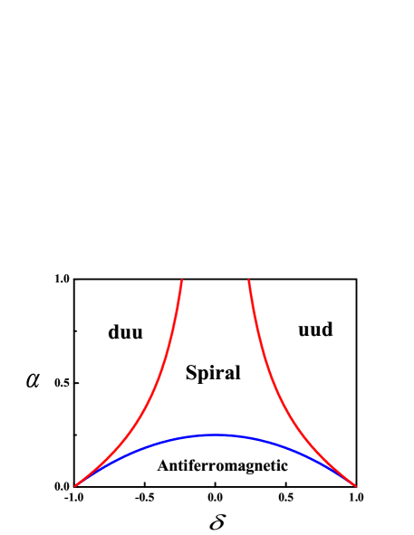
Figure 5: (Color online). The classical ground state Phase diagram of the dimerized and frustrated chains in $\delta-\alpha$ plane. The antiferromagnetic is separated from spiral by critical line. At $\delta=0$, the spiral phase is separated from antiferromagnetic phass by the critical point $\alpha=0.25$.

Minimizing over the angles $\theta,\theta^{\prime},\phi$ , and $\phi^{\prime}$ gives the following equations

$$\frac{\partial h_{c}}{\partial\theta} = -\frac{S^{2}}{2}\Big{\{}(1-\delta)\sin\theta+2\alpha\big{[}\sin\theta\cos\theta^{\prime}$$

$$- \cos\theta\sin\theta^{\prime}\cos(\phi-\phi^{\prime})\big{]}\Big{\}},$$

$$\frac{\partial h_{c}}{\partial\theta^{\prime}} = -\frac{S^{2}}{2}\Big{\{}(1+\delta)\sin\theta^{\prime}+2\alpha\big{[}\sin\theta^{\prime}\cos\theta$$

$$- \cos\theta^{\prime}\sin\theta\cos(\phi-\phi^{\prime})\big{]}\Big{\}},$$

$$\frac{\partial h_{c}}{\partial\phi} = -\frac{S^{2}}{2}\Big{\{}-2\alpha\sin\theta\sin\theta^{\prime}\sin(\phi-\phi^{\prime})\Big{\}},$$

$$\frac{\partial h_{c}}{\partial\phi^{\prime}} = -\frac{S^{2}}{2}\Big{\{}2\alpha\sin\theta\sin\theta^{\prime}\sin(\phi-\phi^{\prime})\Big{\}}.$$ (19)

We check the possible configurations which can minimize the above equations. By taking arbitrary $(\phi,\phi^{\prime})$, we have the solutions $(\pi,\pi),(0,0)$ that are related to the antiferromagnetic and ferromagnetic states respectively. We have also the solutions $(\pi,0)\rightarrow(\downarrow,\uparrow,\uparrow)$ and $(0,\pi)\rightarrow(\uparrow,\uparrow,\downarrow)$ that are related to the uud and duu states respectively. Spiral phase also exists same as the coplanar case. The stability of different phases in the non-coplanar case is also checked and behaves same as the coplanar case.

III conclusion

To summarize, we have studied the classical ground state magnetic phase diagram of the dimerized and frustrated Heisenberg chain using LK cluster method. In coplanar case and in the absence of dimerization effect this approach could detect antiferromagnetic(ferromagnetic) and spiral phases. We have shown that turning the dimerization yields to remove the degeneracy between two uud and duu phases. We have argued that in the ground state phase diagram of the system there are first order transition lines. These lines separate spiral and uud or duu phases. On the other hand two second order phase transition points also exist, which separate antiferromagnetic(ferromagnetic) and spiral phases. By helping this approach we have calculated the spiral exact critical exponent $\varepsilon=1/2$.

In order to generalize our treatment, we have considered the non-coplanar case and checked its phases by LK cluster method. Our calculations revealed that in the non-coplanar case classical phase diagram consist of antiferromagnetic or ferromagnetic depend on nearest neighbor coupling, duu and uud phases which are still non-degenerate and spiral phase. Finally, one of the main achievement of our work which should be highlighted is that in the both coplanar and non-coplanar cases, the spiral state is stable in the classical phase diagram for $\delta\neq 0$.

References

- (1) J. M. Luttinger and L. Tisza Phys. Rev. 70, 954 (1946); J. M. Luttinger and Laszo Tisza Phys. Rev. 72, 257 (1947) .
- (2) R.J. Baxter, Exactly solved models in statistical mechanics, London, Academic Press, (1982).
- (3) E. H. Lieb, Physical Review 162, 162-172 (1967).
- (4) B. Sutherland, J. Math. Phys. 11, 3183 (1970).
- (5) T. Kaplan, Phys. Rev. B 80, 012407 (2009); T. Kaplan, Phys. Rev. B 80, 229906 (2009).
- (6) D. H. Lyons and T. A. Kaplan, J. Phys. Chem. Solids, 25, 645 (1964).
- (7) L. X. Hayden, T. A. Kaplan and S. D. Mahanti, Phys. Rev. Lett. 105, 047203 (2010).
- (8) J. Vahedi and S. Mahdavifar, in prepration.
- (9) B. S. Shastry and B. Sutherland, Phys. Rev. Lett. 47, 964 (1981).
- (10) R. Chitra, S. Pati, H. R. Krishnamurthy, D. Sen, and S. Ramasesha, Phys. Rev. B, 52, 6581 (1995).
- (11) S. Pati, R. Chitra, D. Sen, H. R. Krishnamurthy and S. Ramasesha, Europhys. Lett., 33, 707 (1996).
- (12) T. Nakamura and S. Takada, Phys. Rev. B 55, 14413 (1997).
- (13) G. Bouzerar, A. P. Kampf and G. I . Japaridze, Phys. Rev. B 58, 3117 (1998).
- (14) D. Controzzi, C. Degli Esposti Boschi, F. Ortolani and S. Pasini, Phys. Rev. B, 72, 172409 (2005).
- (15) M. Kumar, S. Ramasesha and D. Sen, Z. G. Soos, Phys. Rev. B 75, 052404 (2007).
- (16) S. Takayoshi and M. Oshikawa arXiv:1201.2030v1
- (17) F. D. M. Haldane, Phys. Rev. B 25, 4925 (1982).
- (18) K. Okamoto and K. Nomura, Phys. Lett. A 169, 433 (1992).
- (19) I. Affleck and F. D. M. Haldane, Phys. Rev. B 36, 5291(1987).
- (20) A. Kolezhuk, R. Roth, and U. Schollwock, Phys. Rev. Lett.77, 5142 (1996).
- (21) S. Mahdavifar and A. Akbari, J. Phys. Soc. Jpn 77, 024710 (2008).
- (22) S. Mahdavifar, Eur. phys. J. B 77, 77 (2010).