Anisotropic flow in striped superhydrophobic channels
Abstract
We report results of dissipative particle dynamics simulations and develop a semi-analytical theory of an anisotropic flow in a parallel-plate channel with two superhydrophobic striped walls. Our approach is valid for any local slip at the gas sectors and an arbitrary distance between the plates, ranging from a thick to a thin channel. It allows us to optimize area fractions, slip lengths, channel thickness and texture orientation to maximize a transverse flow. Our results may be useful for extracting effective slip tensors from global measurements, such as the permeability of a channel, in experiments or simulations, and may also find applications in passive microfluidic mixing.
I Introduction
Textured surfaces play a major role in microfluidics, since the high surface to volume ratio enhances fluid-surface interactions Stone et al. (2004). An important class of phenomena involve “transverse” hydrodynamic couplings in anisotropic channels, where an applied pressure gradient or shear rate in one direction generates flow in a different direction, with a nonzero perpendicular component. Transverse hydrodynamic couplings in pressure-driven flow through a textured microchannel were analyzed theoretically Stroock et al. (2002); Ajdari (2001); Wang (2003); Bazant and Vinogradova (2008) and applied to passive chaotic mixing in a herringbone grooved channel Stroock et al. (2002); Stroock and McGraw (2004). Such microfluidic devices have also recently been used to separate or concentrate suspended particles Gao and Gilchrist (2008).
Here we deal with a special (and different) type of surface textures, namely a superhydrophobic (SH) surface in the Cassie state, where air micro- and nanobubbles are favored, and can generate a number of amazing properties Quéré (2005), including a very large liquid slippage Bocquet and Barrat (2007); Vinogradova and Belyaev (2011). Such a slip also occurs at smooth hydrophobic surfaces Vinogradova (1999); Lauga et al. (2007), but with a relatively low amplitude, characterized by a slip length (extrapolated distance on which the liquid velocity vanishes) of the orders of tens of nm or smaller Vinogradova and Yakubov (2003); Cottin-Bizonne et al. (2005); Joly et al. (2006); Vinogradova et al. (2009). Due to a local slip length of tens of m over gas regions the dramatic enhancement of slip at such a superhydrophobic surface could be achieved Choi et al. (2006); Joseph et al. (2006); Tsai et al. (2009); Rothstein (2010) and may dramatically reduce viscous drag in a channels.
Directional SH textures generate the anisotropy of effective slip, which becomes a tensor, , represented by a symmetric, positive definite matrix
| (1) |
diagonalized by a rotation with angle
| (2) |
The tensor formalism allows us to easily change the orientation of a texture, once a problem has been solved for a given geometry. For all anisotropic surfaces its eigenvalues and correspond to the fastest (greatest forward slip) and slowest (least forward slip) orthogonal directions Bazant and Vinogradova (2008). Note that the concept of an effective slip length tensor is applied for an arbitrary channel thickness Schmieschek et al. (2012), being a global characteristic of a channel Vinogradova and Belyaev (2011). A corollary of this is that the eigenvalues depend not only on the parameters of the heterogeneous surfaces (such as local slip lengths, fractions of phases, and a texture period), but also on the channel thickness. However for a thick (compared to a texture correlation length) channel they become a characteristics of a heterogeneous interface solely Bazant and Vinogradova (2008). In the general case of any direction , the anisotropy of effective slip means that the flow past such surfaces becomes misaligned with the driving force. Therefore, anisotropic SH textures can potentially be used to generate transverse hydrodynamic flow, which is of obvious fundamental and practical interest. However, most of the prior theoretical work has focused on the maximization of the effective slip, and general principles to optimize transverse phenomena have received much less attention and have not yet been established.
Computer simulations might be expected to shed some lights on a flow past anisotropic surfaces. Earlier Molecular Dynamics (MD) simulations observed how modulations of hydrophobicity induce (small) variations in local slip at channels of finite thickness, but did not attempt to relate these to effective boundary conditions Qian et al. (2005); Hendy et al. (2005). In efforts to better understand the connection between the parameters of the texture and the effective slip lengths, several other groups have been performed MD simulations of the flow past striped anisotropic surfaces. Most of these studies considered a thick channel geometry, and focused only on calculating eigenvalues of the effective slip-length tensor Cottin-Bizonne et al. (2004); Priezjev et al. (2005). There are however two simulations which are directly relevant. Recent work Priezjev (2011) studied the dependence of a ratio of transverse and forward effective slip velocities on the flow orientation in a thick channel, but it did not explore the situation of a finite channel thickness. It has been found that the theoretical predictions based on a concept of tensorial slip consistently overestimated the results of MD simulations, which has been attributed to the fact that the stripe width was comparable to the molecular size. Other recent simulations Schmieschek et al. (2012) used the lattice-Boltzmann (LB) approach to calculate a flow in an asymmetric channel (i.e. with one SH and one no-slip hydrophilic wall) of arbitrary thickness. This study confirmed that the eigenvalues of the effective slip-length tensor depend on the gap and validated the concept of tensorial slip. An excellent agreement of LB results with a continuous theory gave a strong support to macroscopic arguments. However, no attempts have been made to simulate the deflection of flow from the main direction, which for an asymmetric SH channel was not expected to be very dramatic Vinogradova and Belyaev (2011).
The goal of the present paper is to provide some general theoretical results to guide the optimization of transverse hydrodynamic phenomena in a symmetric channel with two aligned striped SH walls. In the case of thin channels, symmetric striped walls provide rigorous upper and lower bounds on the effective slip over all possible two-phase patterns Feuillebois et al. (2009) and are expected to generate very strong transverse flow Feuillebois et al. (2010), which could lead to very efficient mixing upon spatial modulation of the texture. Here we consider a channel of arbitrary thickness, and optimize its orientation to maximize pressure-driven transverse flow. Our consideration is based on theoretical analysis and dissipative particle dynamics (DPD) simulations. By using relatively wide stripes as compared with a recent MD study Priezjev (2011) we find that our results in a very good quantitative agreement with the macroscopic theory.
II Model and general consideration
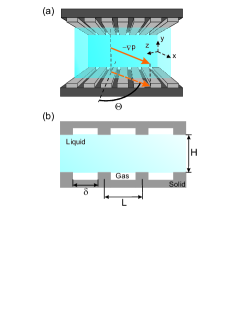
We consider a channel consisting of two equal symmetric SH walls located at and and unbounded in the and directions as sketched in Fig. 1. The origin of the coordinates is placed in the plane of a liquid-gas interface at the center of the gas sector. The axis is defined along the pressure gradient. As in previous publications Bocquet and Barrat (2007); Belyaev and Vinogradova (2010a); Priezjev et al. (2005); Priezjev (2011); Asmolov et al. (2011), we model SH plates as flat interfaces with no meniscus curvature, so that they appear as being perfectly smooth with a pattern of boundary conditions. The latter are taken as no-slip () over solid/liquid areas and as partial slip () over gas/liquid regions. In this idealization, by assuming a flat interface, we neglect an additional mechanism for a dissipation connected with the meniscus curvature Davis and Lauga (2009); Sbragaglia and Prosperetti (2007). The fraction of the solid/liquid areas is denoted as , and that of the gas/liquid areas as .
The flow is governed by the Stokes equations
| (3) |
where u is the velocity vector, and the average pressure gradient is always aligned with the -axis direction:
| (4) |
The local slip boundary conditions at the walls have the form
| (5) |
In addition, a symmetry condition applies at the mid-channel,
| (6) |
Here the local slip length at the SH surface is generally a function of both lateral coordinates.
The effective slip length at the SH surface is defined as usual,
| (7) |
where denotes the average value in the plane . It can equivalently be defined via a permeability tensor
| (8) |
In the linear response regime, the averaged flow rate, , is proportional to via the permeability tensor, k:
| (9) |
which may be rewritten as
| (10) | |||||
| (11) |
Integrating the velocity profile across the channel we obtain
| (12) |
or
| (13) | |||||
| (14) |
The above formula are valid regardless of the thickness of the symmetric SH channel and are independent of the details of the textured surface. There could be arbitrary patterns of local slip lengths, and the latter could itself be a spatially varying tensor.
III Theory for striped patterns
To illustrate the general model, in this section we focus on flat patterned SH surfaces consisting of aligned periodic stripes, where the local (scalar) slip length varies only in one direction. We mostly follow the approach developed before Schmieschek et al. (2012), but apply the method to a symmetric channel situation as sketched in Fig. 1, where the surfaces are covered with arrays of gas/liquid stripes with width and period . Thus, and , respectively.
For transverse stripes, the flow is two-dimensional , , and . For longitudinal stripes, we also have a plane flow: , . As the problem is linear in v, we seek for a solution of the form
| (15) |
where is the velocity of the usual no-slip parabolic Poiseuille flow
| (16) |
and is the SH slip-driven superimposed flow.
III.1 Longitudinal stripes
In this situation the problem is homogeneous in -direction (). The slip length is periodic in with period . The elementary cell is determined as at , and at . In this case the velocity has only one nonzero component, which can be determined by solving the Laplace equation
| (17) |
The Fourier expansion of a periodic solution satisfying (6) reads
| (18) |
with . The sine terms vanish due to symmetry. Applying (5) we then obtain a trigonometric dual series:
| (19) | |||
| (20) |
where
The dual series (19), (20) provide a complete description of the hydrodynamic flow and the effective slip length (due to Eq. (12)) in the longitudinal direction, given all the stated assumptions. These equations can be solved numerically, but exact results can be obtained in the limits of thin and thick channels.
For a thin channel, , we can use that . By substituting this expression into (19) and keeping only values of the first non-vanishing order, we find
| (21) |
This is an exact solution, representing a rigorous upper Wiener bound on the effective slip over all possible two-phase patterns in a thin channel Feuillebois et al. (2009).
III.2 Transverse stripes
To describe a two-dimensional flow in this case we use a standard technique and introduce a stream function and the vorticity vector . Thus, the velocity field is represented by , and the vorticity vector, , has only one nonzero component, which is equal to
| (23) |
The solution can then be presented as the sum of the base flow with homogeneous no-slip condition and its perturbation caused by the presence of stripes as
| (24) | |||||
| (25) |
The problem for and reads
| (26) |
which can be solved with respect to the BC (5)-(6) and an additional condition that reflects our definition of the stream function:
| (27) |
The general solution reads
| (28) | |||||
| (29) |
The following relations between Fourier coefficients may be established:
Again we obtain a dual series problem, which is similar to (19) and (20):
| (30) | |||
| (31) |
Here,
| (32) | |||||
| (33) |
and
| (34) |
In the limit of a thin channel one has , from which it follows that
| (35) |
This exact equation represents a rigorous lower Wiener bound on the effective slip over all possible two-phase patterns in a thin symmetric channel Feuillebois et al. (2009).
For completeness we discuss again the two limiting situations:
| (36) |
| (37) |
III.3 Transverse flow
The tensorial nature of the effective slip is physically due to secondary flows transverse to the direction of the applied pressure gradient. Now we focus on transverse flow optimization, which is necessary for a passive mixing in a symmetric SH channel. Our aim is to optimize the texture, channel thickness and the angle between the directions of stripes and the pressure gradient, so that is as large as possible.
Following the approach Vinogradova and Belyaev (2011), one can derive
| (39) |
Consider now the tilt angle, , confined between and and rewrite Eq. (39) as
| (40) |
where , and . By evaluating , we find that the maximum occurs at
| (41) |
and its value is
| (42) |
In the limit of a thick channel, , (owing to the fact that is limited by the local slip length and independent of for that case), and Eq. (41) gives
| (43) |
and, correspondingly,
| (44) |
Therefore, the mixing in a thick symmetric SH channel would be not very efficient. According to our formula, to maximize an efficient strategy would be to use striped textures with largest physically possible and a very low fraction of a solid phase, .
When the channel is thin, , the interplay between and gives two possibilities. First, if , the slip length is isotropic, , and , . Therefore, again , yet the value
| (45) |
is negligible. Then, for we get
Substitution of these expressions into Eqs. (41) and (42) gives
| (46) |
| (47) |
Since is maximal for , the direction of optimal inflow angle is
| (48) |
which coincides with the results of Feuillebois et al. (2010) derived by using a different method.
IV Simulation method
Our simulations are done using Dissipative Particle Dynamics (DPD), an established method for mesoscale fluid simulations, which is fully off-lattice and particle based and naturally includes thermal fluctuations Koelman and Hoogerbrugge (1993); Español and Warren (1995); Groot and Warren (1997). More specifically, we use a DPD version without conservative interactions, and combine that with a tunable-slip method that allows one to implement arbitrary hydrodynamic boundary conditions Smiatek et al. (2008). The detailed implementation of the tunable-slip method can be found in Ref. Smiatek et al. (2008). In the following we only give a brief description and introduce the simulation parameters.
In the tunable-slip boundary approach, the interaction between the channel walls and the fluid particles has two contributions. The first is a Weeks-Chandler-Andersen (WCA) interaction to mimic the impermeable surfaces,
| (49) |
where is the distance between the fluid particle and the wall. This is just a Lennard-Jones interaction with a cutoff at the potential minimum, corresponding to the pure repulsive part of the potential. In the following, the WCA parameters will set our simulation units, i.e., the energy unit and the length unit . The third unit is the particle mass . The second part of the wall-fluid interaction is a coarse-grained friction force, which is introduced in a similar spirit than the DPD approach. Specifically, the effect of the wall friction on -th particle is implemented by introducing a pair of Langevin-type forces,
| (50) |
The dissipative contribution has the form
| (51) |
This force is proportional to the relative fluid velocity with respect of the wall, and the proportionality factor is the local viscosity . The position-dependent function is a monotonically decreasing function of the wall-particle separation, and vanishes when the fluid particle is further away from the wall than a cutoff distance . In our simulations, we take to decrease linearly from 1 to 0. The prefactor characterizes the strength of the wall friction and can be used to tune the value of the slip length. A random force obeying the fluctuation-dissipation theorem is required to ensure the correct equilibrium statistics,
| (52) |
where each component of is a Gaussian distributed random variable with zero mean and unit variance.
The simulations are carried out using the open source simulation package ESPResSo Limbach et al. (2006). All simulations are performed with a time step , and the temperature of the system is set at . The fluid has a density . Fluid particles have no conservative interactions, they interact only with the dissipative part of the DPD interactions, The DPD interaction parameter is chosen at and the cutoff radius is , which results in a shear viscosity of .
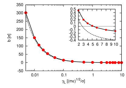
The slip length can be calculated analytically as a function of the simulation parameters (the wall friction parameter and cutoff ) to a very good approximation. For the purpose of this work, however, we need highly accurate values for both and the position of the hydrodynamic boundary, therefore we determined it with the method described in Ref. Smiatek et al. (2008) by simulating plane Poiseuille flow and plane Couette flow. Fig. 2 shows the relation between the slip length and the wall friction parameter , for a wall interaction cutoff . By setting the wall friction parameter , we can adjust the slip length to arbitrary values. The no-slip boundary condition is implemented with . The position of the hydrodynamic boundary, was determined to be away from the simulation wall.
For simulations of patterned surfaces, we use a box of . The two impermeable surfaces lie parallel to the -plane and are separated by a distance . Periodic boundary conditions are assumed in the plane in the directions parallel and perpendicular to the stripes. We have tested that increasing the simulation box does not change the outcome. The surfaces are decorated by alternating no-slip and partial slip stripes. The pattern has a periodicity of . The wall friction parameters are chosen , which implements a no-slip boundary condition, and , corresponding to . A simulation system is completely specified by the following parameters: (, , , ).
The simulation starts with randomly distributed DPD particles. An external body force is assigned to each particle to mimic the pressure gradient. The amplitude of the force is adjusted such that the maximum shear rate at the surface is . Small shear rates are necessary to avoid shear-rate dependencies of the slip length Thompson and Troian (1997) and reduce inertia effects. With these parameters, typical Reynolds numbers in our system are still of order 10, which is much larger than typical values in microfluidic setups. To reach realistic Reynolds numbers, one would have to reduce the body force by four orders of magnitude. Unfortunately, the necessary simulation time for gathering data with sufficiently good statistics would then increase prohibitively, since the values of the relevant observables become very small and the correlation times increase with . Test runs with selective parameters were performed using a smaller body force, but the results did not change significantly. Therefore, we chose to work at these relatively high Reynolds numbers (we are still deeply in the laminar regime), and tolerate slight inertia effects, which we will discuss further below.
One important criterion for a correct simulation of the pressure-driven flow is a constant density profile. Fig. 3(a) shows an example of the fluid density profile for . The channel has a thickness of . The periodicity of the striped pattern is , and the partial-slip part has a slip length of and area fraction . The fluid density is uniform in the middle of the channel. and drops to zero in the proximity of the wall due to the repulsive interaction of the wall on the fluid particles. This leads to a physical wall position which is approximately away from the simulation wall. The quoted value of channel thickness is the separation between the physical walls. In contrast to earlier MD simulations Priezjev et al. (2005), there are no molecular layering effects and density oscillations near the walls, because our DPD particles have no conservative interactions.
(a)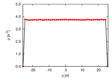 (b)
(b)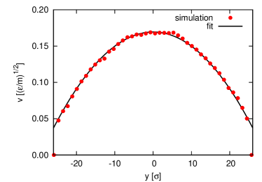
Fig. 3(b) shows the averaged velocity profile for the same system. The system is allowed to run up to time steps to reach a steady state, and the velocity profile is then averaged over long time intervals (up to time steps) with horizontal bins of thickness . Close to the wall, the velocity is zero because no particles are present in that region. In the middle of the channel, the velocity profile exhibits a parabolic shape, such that we can fit the velocity to a plane Poiseuille flow and obtain an effective slip length. The fitting function we used is
| (53) |
where is the external force applied to each DPD particle to induce the pressure gradient. For the position of the hydrodynamic boundary , we use the value obtained from simulations for homogeneous surfaces ( from the simulation wall). We assume that the position of the hydrodynamic boundary remains the same for striped surfaces. The values of and are then computed with Eqs. (13)-(14).
V Results and Discussion
In this section, we present the DPD simulation results and compare them with predictions from the continuous theory. Throughout the section, we use striped patterns with periodicity and slip length on the slippery areas. We study the effect of varying the film thickness , the angle between the applied force and the stripes, and the area fraction of slippery areas.
(a)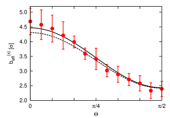 (b)
(b)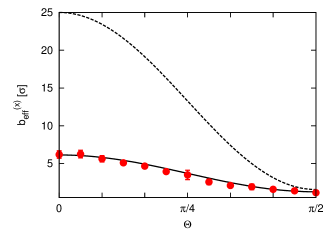
We start with varying in a system where the stick and slip areas are equal, , which corresponds to maximum transverse flow in a thin channel situation Feuillebois et al. (2010). Fig. 4 shows the results for the effective downstream slip lengths, , as obtained from Poiseuille fits (53) to the component of the velocity , for two values of the channel thickness, and . We emphasize that in both cases we formally have an intermediate channel situation, since . The error bars have been obtained from averaging over five independent runs. Since we model an infinitely extended slit by virtue of applying periodic boundary conditions in the plane, the downstream slip length in our system, , corresponds to . (In channels that are confined in the direction, a transverse pressure builds up that renormalizes Bazant and Vinogradova (2008).) Fig. 4 also includes a theoretical curve calculated using Eq. (1), which can be explicitly written as
| (54) |
Here, the eigenvalues of the slip-length tensor are obtained by numerical solution of the dual series, using the procedure described in Ref. Schmieschek et al. (2012). Also included in Fig. 4 (dashed curves) are the components of the effective slip length tensor calculated in the limit of thick [Fig. 4(a)] and thin [Fig. 4(b)] channels. These indicate the range of in this (symmetric) channel geometry.
The simulation data are in a good agreement with theoretical predictions, confirming the anisotropy of the flow and the validity of the concept of a tensorial slip for arbitrary channel thickness Schmieschek et al. (2012). Most notably, the effective slip is larger for thinner channels, somewhat in contrast to previous findings for asymmetric channels, where the magnitude of the effective slip length in a thin gap was much smaller than that in a thick channels Schmieschek et al. (2012); Asmolov et al. (2011); Belyaev and Vinogradova (2010a). This means that transverse hydrodynamic phenomena should be enhanced in thinner channels.
(a)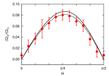 (b)
(b)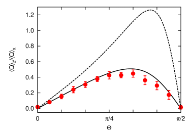
The development of transverse flow is illustrated in Fig. 5, where the data for the ratio of the measured averaged longitudinal and transverse flow rates at different are presented and compared with the theoretical prediction of Eq. (39). The simulation data and the theoretical prediction agree quite well. There are some discrepancies at intermediate angles , where the simulation data for are smaller than predicted by theory. These slight deviations are most likely a result of the finite Reynolds numbers, which are of order in the present simulations as discussed in Section IV. When increasing the bulk force and hence the average flow velocities, the deviations increase, thus they will presumably vanish in the Stokes limit. A pressure gradient in eigendirections cannot produce any transverse flow (and the tensorial boundary condition reduces to a scalar one), which is well seen in Fig. 5. In all other situations the direction of flow is different from that of the pressure gradient. The maximum value of is smaller for the larger channel (Fig. 5(a)). In this case, this maximum is reached at , which agrees with theoretical calculations made with Eq. (43) for a thick channel. For the thinner channel, however, the maximal is observed at larger (Fig. 5(b)), also in agreement with the theory (see discussion above). An important conclusion from these results is that the surface textures which optimize transverse flow differ significantly from those optimizing effective (forward) slip. Similar predictions have been made for other channel configurations Vinogradova and Belyaev (2011); Feuillebois et al. (2010).
Next we examine the effect of varying the fraction of slippery gas/liquid phase, . Fig. 6 shows the eigenvalues, and , of the slip-length tensor as a function of . The two data sets again correspond to different thickness of the channel, and . The results clearly demonstrate that is the main factor determining the value of effective slip, which significantly increases with the fraction of the slippery sectors. The theoretical curves match the simulation data very nicely.
(a)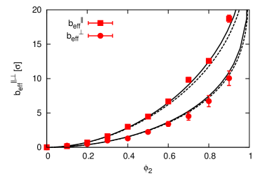 (b)
(b)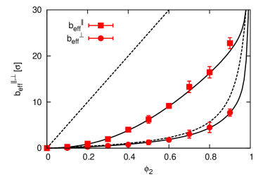
To illustrate the effect of on the transverse phenomena, we now fix and measure . The simulation data presented in Fig. 7 show that the maximum value of is observed at and depends on the channel thickness. As discussed above, results in maximum transverse flow in a thin channel (thin compared to the period of the texture) Feuillebois et al. (2010). For thick channels, the continuum theory predicts maximal transverse flow at . The simulation data, obtained for two values of , confirms these trends. Fig. 7 also illustrates that transverse phenomena are more efficient in a thinner channel. The data sets in Fig. 7 are in quantitative agreement with predictions of the continuum theory. Only for the thick channels and do we observe slight deviations, which again presumably reflect inertia effects.
(a)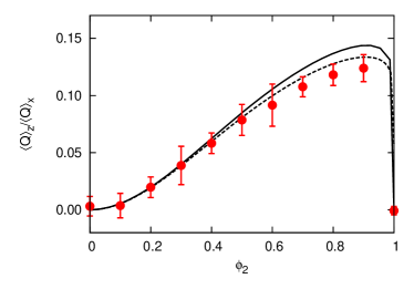
(b)
The simulation and theoretical data presented in Figs. 4 and 6 show that the eigenvalues of the slip-length tensor depend on the channel thickness , in agreement with earlier predictions Schmieschek et al. (2012). To examine this dependence in more detail, we now fix and vary in a large range. The smallest gap was taken to be , for smaller gaps the velocity profile can no longer be resolved satisfactorily. The largest thickness was chosen to be equal to . The eigenvalues of the slip-length tensor are shown in Fig. 8. Also included are continuum theoretical calculations (solid curves) and asymptotic values (dashed curves) expected in the true limits of thin and thick channels. The data show that the longitudinal effective slip decreases with . In contrast, the transverse effective slip increases with , so that the difference between two eigenvalues is largest for thin channels. We remark and stress that the effective slip reaches the asymptotic values predicted for a thick channel already at . A similar observation was made in Schmieschek et al. (2012) for asymmetric channels. This result is remarkable since it suggests that the thick channel limit, where the effective slip is a property of single interfaces and does not depend on , is already reached for channels whose thickness is of the order of the texture period. In practice, this implies that huge simulations with large simulation boxes are not necessary to determine the effective hydrodynamic behavior in such systems. We note however that even for the smallest gaps considered here (), our theoretical and simulation results still deviate strongly from the upper Wiener bound, Eq. (21), although they are very close to the lower Wiener bound, Eq. (35).
(a)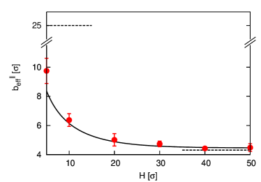 (b)
(b)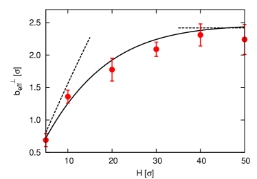
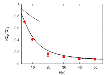
Fig. 9 shows the corresponding simulation and theoretical data for as a function of channel thickness . The stripe texture is the same as in Fig. 8, i.e., , and the tilt angle was chosen . As discussed above, this angle leads to a maximal transverse flow in case of a thick channel, but not in the thin channel situation, where a much larger angle is required to optimize the transverse phenomena. Nevertheless, increases dramatically, when the channel becomes thinner. With our range of parameters, however, we are still well below the limiting value of , which would be expected in case Wiener bounds were attained.
(a)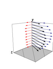 (b)
(b)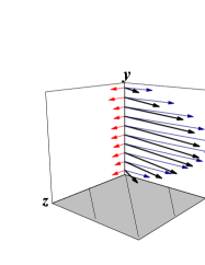 (c)
(c)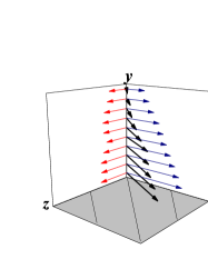 (d)
(d)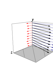
Finally in this section, we show the measured velocity profile in a channel with stripes inclined at the angle with respect to the applied force (Fig. 10). The velocity profile results from superimposed flows in the (forward) and the (transverse) directions (also shown). As above we use [Fig. 10(a)] and [Fig. 10(b)]. The data show that the effective velocity direction is generally misaligned with the force vector, and this effect is much more pronounced for a thin channel due to a larger transverse component of the velocity. The flow has the form of a superimposed no-slip parabolic Poiseuille flow and a slip-driven plug-flow everywhere in the thin channel. In case of a thick channel the flow near the surface is different from that in the center of the channel. To examine this more closely, the short-distance region of the flow from Fig. 10(b) is reproduced in Fig. 10(c), and the central part is shown in Fig. 10(d). These blowups demonstrate that the strong transverse flow due to surface anisotropy is generated only in the vicinity of the wall and tends to disappear far from it, as predicted theoretically Vinogradova and Belyaev (2011) and observed in experiment Ou et al. (2007). The effective velocity profile is ‘twisted’ close to the striped wall.
VI Conclusion
We have investigated pressure-driven flow in a flat-parallel channel with two aligned striped SH surfaces. For this geometry of configuration we propose a semi-analytical theory, which is valid for an arbitrary gap and any local slip length at the slipping areas of the stripes. Analytical results are presented for various important limits, and our approach gives simple analytical formula for an effective slip length in case of stripes that are inclined with respect to a pressure gradient. Furthermore, our theory gives analytical guidance as to how to choose the parameters of the texture and a tilt angle, in order to optimize the transverse flow in different situations. Our theoretical predictions have been compared with results of DPD simulations, which are in a good quantitative agreement with the macroscopic theory. Our results are directly relevant for passive mixing in thin channels and other microfluidic applications. In the future, we hope to augment our analysis to include the possibility of a surface charge patterns, which would help to understand transverse electro-osmotic phenomena. Another fruitful direction could be to consider identical, but misaligned striped walls, where the relative orientation of surfaces could generate additional mechanism of mixing.
Acknowledgments
We are grateful to V. Lobaskin for discussions and advice. This research was supported by the RAS through its priority program ‘Assembly and Investigation of Macromolecular Structures of New Generations’, and by the DFG through SFB-TR6. The simulations were carried out using computational resources at the John von Neumann Institute for Computing (NIC Jülich), the High Performance Computing Center Stuttgart (HLRS) and Mainz University.
References
- Stone et al. (2004) H. A. Stone, A. D. Stroock, and A. Ajdari, Annu. Rev. Fluid Mech. 36, 381 (2004).
- Stroock et al. (2002) A. D. Stroock, S. K. Dertinger, G. M. Whitesides, and A. Ajdari, Anal. Chem. 74, 5306 (2002).
- Ajdari (2001) A. Ajdari, Phys. Rev. E 65, 016301 (2001).
- Wang (2003) C. Y. Wang, Phys. Fluids 15, 1114 (2003).
- Bazant and Vinogradova (2008) M. Z. Bazant and O. I. Vinogradova, J. Fluid Mech. 613, 125 (2008).
- Stroock and McGraw (2004) A. D. Stroock and G. J. McGraw, Phil. Trans. R. Soc. Lond. A 362, 971 (2004).
- Gao and Gilchrist (2008) C. Gao and J. F. Gilchrist, Phys. Rev. E 77, 025301 (2008).
- Quéré (2005) D. Quéré, Rep. Prog. Phys. 68, 2495 (2005).
- Bocquet and Barrat (2007) L. Bocquet and J. L. Barrat, Soft Matter 3, 685 (2007).
- Vinogradova and Belyaev (2011) O. I. Vinogradova and A. V. Belyaev, J. Phys.: Cond. Matter 23, 184104 (2011).
- Vinogradova (1999) O. I. Vinogradova, Int. J. Miner. Proc. 56, 31 (1999).
- Lauga et al. (2007) E. Lauga, M. P. Brenner, and H. A. Stone, Handbook of Experimental Fluid Dynamics (Springer, NY, 2007), chap. 19, pp. 1219–1240.
- Vinogradova and Yakubov (2003) O. I. Vinogradova and G. E. Yakubov, Langmuir 19, 1227 (2003).
- Cottin-Bizonne et al. (2005) C. Cottin-Bizonne, B. Cross, A. Steinberger, and E. Charlaix, Phys. Rev. Lett. 94, 056102 (2005).
- Joly et al. (2006) L. Joly, C. Ybert, and L. Bocquet, Phys. Rev. Lett. 96, 046101 (2006).
- Vinogradova et al. (2009) O. I. Vinogradova, K. Koynov, A. Best, and F. Feuillebois, Phys. Rev. Lett. 102, 118302 (2009).
- Choi et al. (2006) C.-H. Choi, U. Ulmanella, J. Kim, C.-M. Ho, and C.-J. Kim, Phys. Fluids 18, 087105 (2006).
- Joseph et al. (2006) P. Joseph, C. Cottin-Bizonne, J. M. Benoît, C. Ybert, C. Journet, P. Tabeling, and L. Bocquet, Phys. Rev. Lett. 97, 156104 (2006).
- Tsai et al. (2009) P. Tsai, A. M. Peters, C. Pirat, M. Wessling, R. G. H. Lammertink, and D. Lohse, Phys. Fluids 21, 112002 (2009).
- Rothstein (2010) J. P. Rothstein, Annu. Rev. Fluid Mech. 42, 89 (2010).
- Schmieschek et al. (2012) S. Schmieschek, A. V. Belyaev, J. Harting, and O. I. Vinogradova, Phys. Rev. E 85, 016324 (2012).
- Qian et al. (2005) T. Qian, X.-P. Wang, and P. Sheng, Phys. Rev. E 72, 022501 (2005).
- Hendy et al. (2005) S. C. Hendy, M. Jasperse, and J. Burnell, Phys. Rev. E 72, 016303 (2005).
- Cottin-Bizonne et al. (2004) C. Cottin-Bizonne, C. Barentin, E. Charlaix, L. Bocquet, and J.-L. Barrat, Eur. Phys. J. E 15, 427 (2004).
- Priezjev et al. (2005) N. V. Priezjev, A. A. Darhuber, and S. M. Troian, Phys. Rev. E 71, 041608 (2005).
- Priezjev (2011) N. V. Priezjev, J. Chem. Phys. 135, 204704 (2011).
- Feuillebois et al. (2009) F. Feuillebois, M. Z. Bazant, and O. I. Vinogradova, Phys. Rev. Lett. 102, 026001 (2009).
- Feuillebois et al. (2010) F. Feuillebois, M. Z. Bazant, and O. I. Vinogradova, Phys. Rev. E 82, 055301(R) (2010).
- Belyaev and Vinogradova (2010a) A. V. Belyaev and O. I. Vinogradova, Soft Matter 6, 4563 (2010a).
- Asmolov et al. (2011) E. S. Asmolov, A. V. Belyaev, and O. I. Vinogradova, Phys. Rev. E 84, 026330 (2011).
- Davis and Lauga (2009) A. M. J. Davis and E. Lauga, Phys. Fluids 21, 011701 (2009).
- Sbragaglia and Prosperetti (2007) M. Sbragaglia and A. Prosperetti, Phys. Fluids 19, 043603 (2007).
- Belyaev and Vinogradova (2010b) A. V. Belyaev and O. I. Vinogradova, J. Fluid Mech. 652, 489 (2010b).
- Koelman and Hoogerbrugge (1993) J. M. V. A. Koelman and P. J. Hoogerbrugge, Europhys. Lett. 21, 363 (1993).
- Español and Warren (1995) P. Español and P. Warren, Europhys. Lett. 30, 191 (1995).
- Groot and Warren (1997) R. D. Groot and P. B. Warren, J. Chem. Phys. 107, 4423 (1997).
- Smiatek et al. (2008) J. Smiatek, M. Allen, and F. Schmid, Eur. Phys. J. E 26, 115 (2008).
- Limbach et al. (2006) H. Limbach, A. Arnold, B. Mann, and C. Holm, Comp. Phys. Comm. 174, 704 (2006).
- Thompson and Troian (1997) P. A. Thompson and S. M. Troian, Nature 389, 360 (1997).
- Ou et al. (2007) J. Ou, G. R. Moss, and J. P. Rothstein, Phys. Rev. E 76, 016304 (2007).