Classical and quantum massive cosmology for the open FRW universe

Abstract

In an open Friedmann-Robertson-Walker (FRW) space background, we study the classical and quantum cosmological models in the framework of the recently proposed nonlinear massive gravity theory. Although the constraints which are present in this theory prevent it from admitting the flat and closed FRW models as its cosmological solutions, for the open FRW universe, it is not the case. We have shown that, either in the absence of matter or in the presence of a perfect fluid, the classical field equations of such a theory adopt physical solutions for the open FRW model, in which the mass term shows itself as a cosmological constant. These classical solutions consist of two distinguishable branches: One is a contacting universe which tends to a future singularity with zero size, while another is an expanding universe having a past singularity from which it begins its evolution. A classically forbidden region separates these two branches from each other. We then employ the familiar canonical quantization procedure in the given cosmological setting to find the cosmological wave functions. We use the resulting wave function to investigate the possibility of the avoidance of classical singularities due to quantum effects. It is shown that the quantum expectation values of the scale factor, although they have either contracting or expanding phases like their classical counterparts, are not disconnected from each other. Indeed, the classically forbidden region may be replaced by a bouncing period in which the scale factor bounces from the contraction to its expansion eras. Using the Bohmian approach of quantum mechanics, we also compute the Bohmian trajectory and the quantum potential related to the system, which their analysis shows are the direct effects of the mass term on the dynamics of the universe.
PACS numbers: 98.80.-k, 98.80.Qc, 04.50.+h
Keywords: Massive cosmology, Quantum cosmology

1 Introduction

General Relativity (GR) introduced by Einstein began a renaissance in scientific thought which changed our viewpoint on the concept of space-time geometry and gravity. The interpretation of gravitational force as a modification of geometrical structure of space-time made and makes this force distinguishable from other fundamental interactions, although there are arguments which support the idea that the other interactions may also have geometrical origin. Because of the unknown behavior of gravitational interaction at short distances, this distinction may have some roots in the heart of problems with quantum gravity. Therefore, any hope of dealing with such concepts would be in vain unless a reliable quantum theory of gravity can be constructed. In the absence of a full theory of quantum gravity, it would be then useful to describe its quantum aspects within the context of modified theories of gravity. From a field theory point of view, the gravitational force in GR can be represented as a field theory in which the space-time metric plays the role of the fields and the particle that is responsible to propagate gravity is named graviton. Then, naturally in comparison to the other field theories, one may ask about the different properties of such a particle. The answer to this question is deduced by the linearized form of GR and expansion of the space-time metric $g_{\mu\nu}$, around a fixed background geometry $\eta_{\mu\nu}$, as $g_{\mu\nu}=\eta_{\mu\nu}+h_{\mu\nu}$, where $h_{\mu\nu}$ is the field representation of the graviton. Eventually, it is possible to show that the graviton is a massless spin-$2$ particle.

Then, since our knowledge about the behavior of gravity at very long distances is also incomplete, a question arises: Is it possible to consider a small nonvanishing mass for the graviton, i.e., a massive spin-$2$ particle? In the first attempts to deal with this question, it seemed that adding a mass term to the action may be sufficient. This was done by Fierz and Pauli [1]. However, it was shown that by considering the number of degrees of freedom, this model suffers from the existence of a ghost field, the so-called Boulware-Deser ghost [2], after studying the non-linear terms. This fact made massive gravity an abandoned theory for a while. Recently, de Rahm and Gabadadze proposed a new scenario in which they have shown that it is possible to have a ghost-free massive gravity even at the non-linear level [3]. That was a positive signal in this area, and the early results in this subject have been followed by a number of works that address different aspects of massive gravity [4]. As in the case of the other modified theories of gravity, it is important to seek cosmological solutions in the newly proposed massive theory of gravity. This is done by the authors of Ref. [5], who show that the existence of some constraints prevent the theory from having the nontrivial homogeneous and isotropic cosmological solutions. Indeed, what is shown in Ref. [5] is that, beginning with the flat FRW ansatz in the context of massive gravity, the corresponding field equations result in nothing but the Minkowski metric. However, by re-examination of the conditions, the authors of Refs. [6, 7] have shown that, for the open FRW model, this is not the case, and the nonlinear massive gravity admits the open FRW as a compatible solution for its field equations. Another progresses to find the massive cosmologies lie in the field of the bi-metric theories of gravity; see, for instance, Ref. [8] based on the works of Hassan and Rosen [9], in which they show that a bi-metric representation for massive gravity exists.

Our purpose in the present paper is to continue the works of the authors of Ref. [6, 7] in greater detail, based on the Hamiltonian formalism of the open FRW cosmology in the framework of massive gravity. We obtain the solutions to the vacuum and perfect fluid classical field equations and investigate their different aspects, such as the roll of the graviton’s mass as a cosmological constant, the appearance of singularities, and the late time expansion. We then consider the problem at hand in the context of canonical quantum cosmology to see how the classical picture will be modified. Our final results show that the singular behavior of the classical cosmology will be replaced by a bouncing one when quantum mechanical considerations are taken into account. This means that the quantization of the model suggests the existence of a minimal size for the corresponding universe. We shall also study the quantum model by the Bohmian approach of quantum mechanics to show how the mass term exhibits its direct effects on the evolution of the system.

The structure of the paper is as follows. In section 2, we briefly present the basic elements of the issue of massive gravity and its canonical Hamiltonian for a given open FRW universe. In section 3, classical cosmological dynamics is introduced for the vacuum and perfect fluid. Quantization of the model is the subject of section 4, and in section 5, the Bohmian approach of quantum mechanics is applied to the model. Finally, the conclusions are summarized in section 6.

2 Preliminary set-up

In this section, we start by briefly studying the nonlinear massive gravity action presented in Refs. [6, 7] for the open FRW model, where the metric is given by

$$ds^{2}=g_{\mu\nu}dx^{\mu}dx^{\nu}=-N^{2}(t)dt^{2}+a^{2}(t)\left[dx^{2}+dy^{2}+dz^{2}-\frac{|K|(xdx+ydy+zdz)^{2}}{1+|K|(x^{2}+y^{2}+z^{2})}\right],$$ (1)

with $N(t)$ and $a(t)$ being the lapse function and the scale factor, respectively, and $K=-1$ denoting the curvature index. Here we work in units where $c=\hbar=16\pi G=1$. In the massive gravity scenario one considers a metric perturbation as [5, 10]

$$g_{\mu\nu}=\eta_{\mu\nu}+h_{\mu\nu}=\eta_{ab}\partial_{\mu}\phi^{a}(x)\partial_{\nu}\phi^{b}(x)+H_{\mu\nu},$$ (2)

where $\eta_{ab}=\mbox{diag}(-1,1,1,1)$ and $\phi^{a}(x)$ are four scalar fields known as Stückelberg scalars and are introduced to keep the principle of general covariance also in massive general relativity [11]. It is clear that the first term in (2) is a representation of the Minkowski space-time in terms of the coordinate system $(\phi^{0},\phi^{i})$ and thus the tensor $H_{\mu\nu}$ is responsible for describing the propagation of gravity in this space. The action of the model consists of the gravitational part ${\cal S}_{g}$ and the matter action ${\cal S}_{m}$ as

$${\cal S}={\cal S}_{g}+{\cal S}_{m}.$$ (3)

The matter part of the action is independent of the massive corrections to the gravity part. Also, the gravity part can be expressed in terms of the usual Einstein-Hilbert, with an additional correction term coming from the massive graviton; that is [5]

$${\cal S}_{g}=\int\sqrt{-g}\left[R-\frac{m^{2}}{4}{\cal U}(g,H)\right]d^{4}x,$$ (4)

in which all of the modifications due to the mass and also the interactions between the tensor fields $H_{\mu\nu}$ and $g_{\mu\nu}$ are summarized in the potential ${\cal U}(g,H)$. By using ghost-free conditions for the theory in Ref. [11], we propose the following form for the potential term: [10]

$${\cal U}(g,H)=-4\left({\cal L}_{2}+\alpha_{3}{\cal L}_{3}+\alpha_{4}{\cal L}_{4}\right),$$ (5)

where

$$\left\{\begin{array}[]{ll}{\cal L}_{2}=\frac{1}{2}\left(<{\cal K}>^{2}-<{\cal K}^{2}>\right),\\ \\ {\cal L}_{3}=\frac{1}{6}\left(<{\cal K}>^{3}-3<{\cal K}><{\cal K}^{2}>+2<{\cal K}^{3}>\right),\\ \\ {\cal L}_{4}=\frac{1}{24}\left(<{\cal K}>^{4}-6<{\cal K}>^{2}<{\cal K}^{2}>+3<{\cal K}^{2}>^{2}+8<{\cal K}><{\cal K}^{3}>-6<{\cal K}^{4}>\right),\end{array}\right.$$ (11)

in which the tensor ${\cal K}_{\mu\nu}$ is defined as

$${\cal K}^{\mu}_{\nu}(g,H)=\delta^{\mu}_{\nu}-\sqrt{\eta_{ab}\partial^{\mu}\phi^{a}\partial_{\nu}\phi^{b}},$$ (12)

and the notations $<{\cal K}>=g^{\mu\nu}{\cal K}_{\mu\nu}$, $<{\cal K}^{2}>=g^{\alpha\beta}g^{\mu\nu}{\cal K}_{\alpha\mu}{\cal K}_{\beta\nu}$,… are used for the corresponding traces. Now, equations (4)-(12) describe the gravitational part of the action for a massive gravity theory. Since its explicit form directly depends on the choice of scalar fields $\phi^{a}(x)$, it is appropriate to concentrate on this point first. Interesting forms for such fields should involve terms which would describe a suitable coordinate transformation on the Minkowski space-time. In a flat FRW background, for instance, one may select $\phi^{0}=f(t)$ and $\phi^{i}=x^{i}$, as is used in [5]. Here, for the open FRW metric (1), we use the following ansatz proposed in [6]

$$\phi^{0}=f(t)\sqrt{1+|K|x_{i}x^{i}},\hskip 14.22636pt\phi^{i}=\sqrt{|K|}f(t)x^{i}.$$ (13)

Upon substitution of these scalar fields and also the definition of the Ricci scalar into the relations (4)-(12), we are led to a point-like form for the gravitational Lagrangian in the minisuperspace $\{N,a,f\}$ as

$${\cal L}_{g}=-\frac{3a\dot{a}^{2}}{N}-3|K|Na+m^{2}\left(L_{2}+\alpha_{3}L_{3}+\alpha_{4}L_{4}\right),$$ (14)

where

$$\left\{\begin{array}[]{ll}L_{2}=3a\left(a-\sqrt{|K|}f\right)\left(2Na-a\dot{f}-N\sqrt{|K|}f\right),\\ \\ L_{3}=\left(a-\sqrt{|K|}f\right)^{2}\left(4Na-3a\dot{f}-N\sqrt{|K|}f\right),\\ \\ L_{4}=\left(a-\sqrt{|K|}f\right)^{3}\left(N-\dot{f}\right),\end{array}\right.$$ (20)

in which an overdot represents differentiation with respect to the time parameter $t$. It is seen that this Lagrangian does not involve $\dot{N}$, which means that the momentum conjugate to this variable vanishes. In the usual canonical formalism of general relativity, we know this issue as the primary constraint in the sense that the variable $N$ is not a dynamical variable but a Lagrange multiplier in the Hamiltonian formalism. On the other hand, Lagrangian (14) seems to show an additional constraint related to the Stückelberg scalars whose dynamics are encoded in the function $f(t)$. We see that in spite of the common Lagrangians in which the first derivative of the configuration variables are of second order, $\dot{f}$ appears linearly in the Lagrangian (14). Therefore, by computing the momentum conjugate to $f$; that is, $P_{f}=\frac{\partial{\cal L}_{g}}{\partial\dot{f}}$, we obtain

$$P_{f}=-m^{2}(a-\sqrt{|K|}f)\left[3a^{2}+3\alpha_{3}a(a-\sqrt{|K|}f)+\alpha_{4}(a-\sqrt{|K|}f)^{2}\right].$$ (21)

Now, it is clear that this relation is not invertible to obtain $\dot{f}(f,P_{f})$. In such a case, the Lagrangian is said to be singular and the relations like (21), which hinder the inversion, are known as primary constraints. One may use the method of Lagrange multipliers to analyze the dynamics of the system by adding to the Lagrangian all of the primary constraints multiplied by arbitrary functions of time. However, to deal with our constrained system, we act differently and proceed as follows. We vary the Lagrangian (14) with respect to $f$ to obtain

$$\left(\dot{a}-\sqrt{|K|}N\right)\left[|K|(\alpha_{3}+\alpha_{4})f^{2}(t)-2\sqrt{|K|}(1+2\alpha_{3}+\alpha_{4})a(t)f(t)+(3+3\alpha_{3}+\alpha_{4})a^{2}(t)\right]=0.$$ (22)

The solution $\dot{a}=\sqrt{|K|}N$ of this equation is nothing but what we obtain from the variation of the usual Einstein-Hilbert Lagrangian with respect to $N$. Since its counterpart in massive gravity is

$$\dot{a}=\frac{\sqrt{3|K|(\alpha_{3}+\alpha_{4})^{2}+m^{2}a^{2}(t)\left[2(1+\alpha_{3}+\alpha_{3}^{2}-\alpha_{4})^{3/2}-(1+\alpha_{3})(2+\alpha_{3}+2\alpha_{3}^{2}-3\alpha_{4})\right]}}{\sqrt{3}(\alpha_{3}+\alpha_{4})}N,$$ (23)

we cannot accept the relation $\dot{a}=\sqrt{|K|}N$ as a physical solution. Therefore, the constraint corresponding to the dynamic of $f(t)$ shows itself in the equation

$$\left[|K|(\alpha_{3}+\alpha_{4})f^{2}(t)-2\sqrt{|K|}(1+2\alpha_{3}+\alpha_{4})a(t)f(t)+(3+3\alpha_{3}+\alpha_{4})a^{2}(t)\right]=0,$$ (24)

where using the same notation as in [6], its solutions can be written as

$$f(t)=\frac{X_{\pm}}{\sqrt{|K|}}a(t)\Rightarrow\dot{f}=\frac{X_{\pm}}{\sqrt{|K|}}\dot{a},\hskip 14.22636ptX_{\pm}\equiv\frac{1+2\alpha_{3}+\alpha_{4}\pm\sqrt{1+\alpha_{3}+\alpha_{3}^{2}-\alpha_{4}}}{\alpha_{3}+\alpha_{4}}.$$ (25)

As is argued in [6], in the limit where $\alpha_{3}$ and $\alpha_{4}$ are of the order of a small quantity $\epsilon$, the expression of $X_{+}$ goes to infinity while $X_{-}\rightarrow 3/2$. Because of this limiting behavior, we use the subscript $-$ in the following for numerical values of constants with subscript $\pm$. Now we may insert the constraints (25) into the relations (20) to reduce the degrees of freedom of the system and obtain a minimal number of dynamical variables. If we do so, we obtain

$$\left\{\begin{array}[]{ll}L_{2}=3\left(1-X_{\pm}\right)\left[\left(2-X_{\pm}\right)N-\frac{X_{\pm}}{\sqrt{|K|}}\dot{a}\right]a^{3},\\ \\ L_{3}=\left(1-X_{\pm}\right)^{2}\left[\left(4-X_{\pm}\right)N-3\frac{X_{\pm}}{\sqrt{|K|}}\dot{a}\right]a^{3},\\ \\ L_{4}=\left(1-X_{\pm}\right)^{3}\left[N-\frac{X_{\pm}}{\sqrt{|K|}}\dot{a}\right]a^{3},\end{array}\right.$$ (31)

in terms of which the Lagrangian (14) takes its reduced form with only one physical degree of freedom $a$. The momentum conjugate to $a$ is

$$P_{a}=\frac{\partial{\cal L}_{g}}{\partial\dot{a}}=-\frac{6a\dot{a}}{N}+m^{2}\left(\frac{\partial L_{2}}{\partial\dot{a}}+\alpha_{3}\frac{\partial L_{3}}{\partial\dot{a}}+\alpha_{4}\frac{\partial L_{4}}{\partial\dot{a}}\right).$$ (32)

Noting that

$$\frac{\partial L_{2}}{\partial\dot{a}}=3\frac{X_{\pm}}{\sqrt{|K|}}(X_{\pm}-1)a^{3},\hskip 14.22636pt\frac{\partial L_{3}}{\partial\dot{a}}=3\frac{X_{\pm}}{\sqrt{|K|}}(X_{\pm}-1)^{2}a^{3},\hskip 14.22636pt\frac{\partial L_{4}}{\partial\dot{a}}=\frac{X_{\pm}}{\sqrt{|K|}}(X_{\pm}-1)^{3}a^{3},$$ (33)

one gets

$$P_{a}=-6\frac{a\dot{a}}{N}-\frac{C_{\pm}m^{2}}{\sqrt{|K|}}a^{3},\hskip 14.22636ptC_{\pm}\equiv X_{\pm}(1-X_{\pm})\left[3+3\alpha_{3}(1-X_{\pm})+\alpha_{4}(1-X_{\pm})^{2}\right].$$ (34)

Now, the Hamiltonian of the model can be obtained from its standard definition $H=\dot{a}P_{a}-{\cal L}$, with result

$$H_{g}=N{\cal H}_{g}=N\left[-\frac{1}{12a}\left(P_{a}+\frac{C_{\pm}m^{2}}{\sqrt{|K|}}a^{3}\right)^{2}+3|K|a+c_{\pm}m^{2}a^{3}\right],$$ (35)

in which we have defined

$$c_{\pm}=\left(X_{\pm}-1\right)\left[3(2-X_{\pm})+\alpha_{3}(1-X_{\pm})(4-X_{\pm})+\alpha_{4}(1-X_{\pm})^{2}\right].$$ (36)

We see that the lapse function enters in the Hamiltonian as a Lagrange multiplier as expected. Thus, when we vary the Hamiltonian with respect to $N$, we get ${\cal H}_{g}=0$, which is called the Hamiltonian constraint. On a classical level this constraint is equivalent to the Friedmann equation, wherein our problem at hand can be easily checked by comparing it with the equation of motion (4.5) in [6]. On a quantum level, on the other hand, the operator version of this constraint annihilates the wave function of the corresponding universe, leading to the so-called Wheeler-DeWitt equation.

Now, let us deal with the matter field with which the action of the model is augmented. As we have mentioned, the matter part of the action is independent of modifications due to the mass terms. Therefore, the matter may come into play in a common way and the total Hamiltonian can be made by adding the matter Hamiltonian to the gravitational part of (35). To do this, we consider a perfect fluid whose pressure $p$ is linked to its energy density $\rho$ by the equation of state

$$p=\omega\rho,$$ (37)

where $-1\leq\omega\leq 1$ is the equation of the stated parameter. According to Schutz’s representation for the perfect fluid [12], its Hamiltonian can be viewed as (see [13] for details)

$$H_{m}=N\frac{P_{T}}{a^{3\omega}},$$ (38)

where $T$ is a dynamical variable related to the thermodynamical parameters of the perfect fluid and $P_{T}$ is its conjugate momentum. Finally, we are in a position in which can write the total Hamiltonian $H=H_{g}+H_{m}$ as

$$H=N{\cal H}=N\left[-\frac{1}{12a}\left(P_{a}+\frac{C_{\pm}m^{2}}{\sqrt{|K|}}a^{3}\right)^{2}+3|K|a+c_{\pm}m^{2}a^{3}+\frac{P_{T}}{a^{3\omega}}\right].$$ (39)

The setup for constructing the phase space and writing the Lagrangian and Hamiltonian of the model is now complete. In the following section, we shall deal with classical and quantum cosmologies which can be extracted from a theory with the previously mentioned Hamiltonian.

3 Cosmological dynamics: classical point of view

The classical dynamics are governed by the Hamiltonian equations. To achieve this purpose, we divide this section into two parts. We first consider the case in which the matter is absent, i.e., the vacuum, and then include the matter.

3.1 The vacuum classical cosmology

In this case, we can construct the equations of motion by the Hamiltonian equations with use of the Hamiltonian (35). Equivalently, one may directly write the Friedmann equation from the Hamiltonian constraint $H=0$ which, as we mentioned previously, reflects the fact that the corresponding gravitational theory is a parameterized theory in the sense that its action is invariant under time reparameterization. Noting from (34) that

$$\dot{a}=-\frac{N}{6a}\left(P_{a}+\frac{C_{\pm}m^{2}}{\sqrt{|K|}}a^{3}\right),$$ (40)

equation (35) gives

$$3a\dot{a}^{2}-3|K|a=c_{\pm}m^{2}a^{3},$$ (41)

in which we have chosen the gauge $N=1$, so that the time parameter $t$ becomes the cosmic time $\tau$. As is indicated in [6], this equation looks like the Friedmann equation for the open FRW universe with an effective cosmological constant $\Lambda_{\pm}=c_{\pm}m^{2}$ and admits the following solutions

$$a_{\pm}(\tau)=\sqrt{\frac{3}{\Lambda}}\sinh\left(\pm\sqrt{\frac{\Lambda}{3}}(\tau-\tau_{*})\right),$$ (42)

where $\tau_{*}$ is an integration constant and we have taken $\Lambda=c_{-}m^{2}$. For a positive $\tau_{*}$, the condition $a(\tau)\geq 0$ implies that the expressions of $a_{+}(\tau)$ and $a_{-}(\tau)$ are valid for $\tau\geq\tau_{*}$ and $\tau\leq-\tau_{*}$ respectively, such that $a_{\pm}(\tau_{*})=0$. It is seen that the evolution of the corresponding universe with the scale factor $a_{+}(\tau)$ begins with a big-bang-like singularity at $\tau=\tau_{*}$ and then follows an exponential law expansion at late time of cosmic evolution in which the mass term shows itself as a cosmological constant. For a universe with the scale factor $a_{-}(\tau)$, on the other hand, the behavior is opposite. The universe decreases its size from large values of scale factor at $\tau=-\infty$ and ends its evolution at $\tau=-\tau_{*}$ with a zero size. In figure 1 we have plotted theses scale factors for typical values of the parameters. As this figure shows, although the behavior of $a_{+}(\tau)$ ($a_{-}(\tau)$) is like a de Sitter ($a(\tau)\sim e^{\sqrt{\Lambda/3}\tau}$) universe at $\tau\rightarrow\infty$ ($\tau\rightarrow-\infty$), in spite of the de Sitter, it begins (ends) its evolution with a singularity. In summary, what we have shown previously is that in the framework of an open FRW background geometry, the vacuum solutions of the massive theory are equivalent to the solutions of the usual GR with a cosmological constant. Accordingly, the zero-size singularity of both theories has the same nature. In this sense we would like to emphasize that the metric (1) with the scale factor (42) is indeed a section of the de Sitter hyperboloid

$$-T^{2}+X^{2}+Y^{2}+Z^{2}+W^{2}=1,$$ (43)

embedded in a $5$-dimensional Minkowski space

$$ds^{2}=-dT^{2}+dX^{2}+dY^{2}+dZ^{2}+dW^{2}.$$ (44)

To see this, one may parameterize the hyperboloid in terms of the spherical coordinates $(r,\theta,\phi)$ as [14]

$$\left\{\begin{array}[]{ll}T=\sqrt{1+r^{2}}\sinh\tau,\\ \\ X=\cosh\tau,\\ \\ Y=r\sinh\tau\cos\phi\cos\theta,\\ \\ Z=r\sinh\tau\cos\phi\sin\theta,\\ \\ W=r\sinh\tau\sin\phi,\end{array}\right.$$ (54)

which, upon substitution into the metric (44), yields the open FRW metric with the scale factor $a(\tau)=\sinh\tau$. This means that the point $a=0$ can be viewed as a coordinate singularity. However, we have to note that in the presence of any kind of matter field the point $a(\tau_{*})=0$ represents a true singularity. Thus, our following analysis to quantize the model is based on the minisuperspace coordinate system in terms of which the dynamical representation of the metric, i.e. (1), is written.

In the next section, we shall see how the previous picture may be modified when one takes into account quantum mechanical considerations.

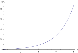
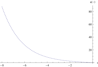
Figure 1: The figures show the evolutionary behavior of the universes based on (42). We have used the numerical values $\Lambda=1$ and $\tau_{*}=0$.

3.2 Perfect fluid classical cosmology

Now, we assume that a perfect fluid in its Schutz’s representation is coupled with gravity. In this case the Hamiltonian (39) describes the dynamics of the system. The equations of motion for $T$ and $P_{T}$ read as

$$\dot{T}=\{T,H\}=\frac{N}{a^{3\omega}},\hskip 14.22636pt\dot{P_{T}}=\{P_{T},H\}=0.$$ (55)

A glance at the above equations shows that with choosing the gauge $N=a^{3\omega}$, we shall have

$$N=a^{3\omega}\Rightarrow T=t,$$ (56)

which means that variable $T$ may play the role of time in the model. Therefore, the Friedmann equation $H=0$ can be written in the gauge $N=a^{3\omega}$ as follows

$$3\dot{a}^{2}=3|K|a^{6\omega}+\Lambda a^{6\omega+2}+P_{0}a^{3\omega-1},$$ (57)

where we take $P_{T}=P_{0}=\mbox{const.}$ from the second equation of (55). Since it is not possible to find the analytical solutions of the above differential equation for any arbitrary $\omega$, we present its solutions only in some special cases.

$\bullet$ $\omega=-\frac{1}{3}$: cosmic string. In this case we obtain

$$a(t)=\left[\frac{\Lambda}{3}(t-t_{0})^{2}-\frac{P_{0}+3|K|}{\Lambda}\right]^{1/2},$$ (58)

where $t_{0}$ is an integration constant. We see that the evolution of the universe based on (58) has big-bang-like singularities at $t=t_{0}\pm t_{*}$ where $t_{*}=\frac{\sqrt{3(P_{0}+3|K|)}}{\Lambda}$. Indeed, the condition $a^{2}(t)\geq 0$ separates two sets of solutions $a^{(I)}(t)$ and $a^{(II)}(t)$, each of which is valid for $t\leq t_{0}-t_{*}$ and $t\geq t_{0}+t_{*}$, respectively. For the former, we have a contracting universe which decreases its size according to a power law relation and ends its evolution in a singularity at $t=t_{0}-t_{*}$, while for the latter, the evolution of the universe begins with a big-bang singularity at $t=t_{0}+t_{*}$ and then follows the power law expansion at late time of cosmic evolution.

One may translate these results in terms of the cosmic time $\tau$. Using its relationship with the time parameter $t$ in this case, that is, $d\tau=a^{-1}(t)dt$, we are led to

$$a(\tau)=\left\{\begin{array}[]{ll}a^{(I)}(\tau)=\frac{1}{\sqrt{12\Lambda}}\left[e^{-\sqrt{\frac{\Lambda}{3}}(\tau-\tau_{0})}-3(P_{0}+3|K|)e^{\sqrt{\frac{\Lambda}{3}}(\tau-\tau_{0})}\right],\hskip 14.22636pt\tau\leq\tau_{0}-\tau_{*},\\ \\ \\ a^{(II)}(\tau)=\frac{1}{\sqrt{12\Lambda}}\left[e^{\sqrt{\frac{\Lambda}{3}}(\tau-\tau_{0})}-3(P_{0}+3|K|)e^{-\sqrt{\frac{\Lambda}{3}}(\tau-\tau_{0})}\right],\hskip 14.22636pt\tau\geq\tau_{0}+\tau_{*},\\ \end{array}\right.$$ (63)

where $\tau_{*}=\frac{1}{2}\sqrt{\frac{3}{\Lambda}}\ln 3(P_{0}+3|K|)$. Again, it is seen that there is a classically forbidden region $\tau_{0}-\tau_{*}<\tau<\tau_{0}+\tau_{*}$, for which we have no valid classical solutions. For $\tau\leq\tau_{0}-\tau_{*}$, the universe has a exponential decreasing behavior which ends its evolution in a singular point with zero size at $\tau=\tau_{0}-\tau_{*}$, while in the region $\tau\geq\tau_{0}+\tau_{*}$ it begins with the big-bang singularity at $\tau=\tau_{0}+\tau_{*}$ and then grows exponentially forever.

$\bullet$ $\omega=-1$: cosmological constant. Performing the integration, we get the following implicit relation between $t$ and $a(t)$:

$$\frac{1}{\sqrt{3}(P_{0}+\Lambda)^{2}}\left[-6|K|+(P_{0}+\Lambda)a^{2}\right]\sqrt{3|K|+(P_{0}+\Lambda)a^{2}}=t-t_{0}.$$ (64)

In terms of the cosmic time $\tau$, it is easy to see that this solution returns to (42), in which the cosmological term is replaced by $\Lambda\rightarrow\Lambda+\mbox{cons}.$ This is expected because the solutions (42) were equivalent to an open FRW universe with a cosmological constant. Therefore, adding a new cosmological term (a perfect fluid with $\omega=-1$) only makes a shift in the corresponding cosmological constant.

4 Cosmological dynamics: quantum point of view

In this section we look for the quantization of the model presented above via the method of canonical quantization. As is well known, this procedure is based on the Wheeler-DeWitt equation $\hat{{\cal H}}\Psi=0$, where $\hat{{\cal H}}$ is the operator version of the Hamiltonian constraint and $\Psi$ is the wave function of the universe, a function of the $3$-geometries and the matter fields. As in the case of the classical cosmology, we consider the matter of free and perfect fluid quantum cosmology separately.

Before going to the subject, a remark is in order related to the Hamiltonians (35) and (39). The term in the round bracket in these Hamiltonians is like the Hamiltonian of a charged particle moving in an electromagnetic field. From this analogy, one may define the transformation

$$P_{a}\rightarrow\Pi_{a}=P_{a}+\frac{C_{\pm}m^{2}}{\sqrt{|K|}}a^{3},\hskip 14.22636pta\rightarrow a,$$ (65)

to simplify the form of the classical Hamiltonian. It is clear that this is a canonical transformation both classically and quantum mechanically [15]. Since going back from a new set of variables to the old ones in a classical canonical transformation can be made without any ambiguity, applying this transformation may not be important for the classical dynamics presented in the previous section. In the context of quantum mechanics, on the other hand, the subject is of little difference. The transition to the quantum version of the theory is achieved by promoting observables to operators which are not necessarily commuting. Thus, by replacing the canonical variables $(a,P_{a})$ by their operator counterparts $(\hat{a},\hat{P_{a}}=-id/da)$, we obtain the quantum Hamiltonian

$$\hat{{\cal H}}=-\frac{1}{12}\hat{a}^{-1}\hat{\Pi_{a}}^{2}+...=-\frac{1}{12}\hat{a}^{-1}\left(\hat{P_{a}}+\frac{C_{\pm}m^{2}}{\sqrt{|K|}}\hat{a}^{3}\right)^{2}+...,$$ (66)

where $...$ denotes the terms out of the round bracket in expressions (35) or (39). When calculating the square, it should be noted that the operators $\hat{a}$ and $\hat{P_{a}}$ do not commute. Although the order of these operators does not matter in the classical analysis, quantum mechanically this issue is quite crucial. Indeed, this is the operator ordering problem and, unfortunately, there is no well defined principle which specifies the order of operators in the passage from classical to quantum theory. There are, however, some simple rules which one uses conventionally. If, for instance, we order the products of $\hat{a}$ and $\hat{P_{a}}$ in $\hat{\Pi_{a}}^{2}$ such that the momentum stands to the right of the scale factor, we obtain

$$\hat{\Pi_{a}}^{2}\rightarrow\hat{P_{a}}^{2}+\frac{C_{\pm}^{2}m^{4}}{|K|}a^{6}+2\frac{C_{\pm}m^{2}}{\sqrt{|K|}}\hat{a}^{3}\hat{P_{a}}-3i\frac{C_{\pm}m^{2}}{\sqrt{|K|}}\hat{a}^{2},$$ (67)

in which we have used the commutation relation $[\hat{a},\hat{P_{a}}]=i$. With this expression at hand, there is still another factor ordering ambiguity in the terms $\hat{a}^{-1}\hat{P_{a}}^{2}$ and $\hat{a}^{2}\hat{P_{a}}$ to construct the quantum Hamiltonian (66). As Hawking and Page have shown [16], the choice of different factor ordering will not affect semiclassical calculations in quantum cosmology, so for convenience one usually chooses a special place for it in the special models. However, in general, the behavior of the wave function depends on the chosen factor ordering [17]. In what follows, as one usually does in the minisuperspace approximation to the cosmological models, we work in the framework of a special factor ordering in which, in addition to the expression (67) for $\hat{\Pi_{a}}^{2}$, we also use the orderings $\hat{a}^{-1}\hat{P_{a}}^{2}=\hat{P_{a}}\hat{a}^{-1}\hat{P_{a}}$ and $\hat{a}^{2}\hat{P_{a}}=\hat{a}\hat{P_{a}}\hat{a}$ to make the Hamiltonian hermitian.

4.1 The vacuum quantum cosmology

In this case, with the help of the Hamiltonian (35) and use of the abovementioned choice of ordering, the Wheeler-DeWitt equation reads

$$\left\{\frac{d^{2}}{da^{2}}+\left(-a^{-1}+2i\frac{C_{\pm}}{c_{\pm}}\Lambda a^{3}\right)\frac{d}{da}+\left[\left(36+2i\frac{C_{\pm}}{c_{\pm}}\Lambda\right)a^{2}+12\Lambda a^{4}-\frac{C_{\pm}^{2}}{c_{\pm}^{2}}\Lambda^{2}a^{6}\right]\right\}\Psi(a)=0.$$ (68)

This equation does not seem to have analytical solutions. However, we can get some properties of its solutions in special regions where there is interest in classical and quantum regimes. First of all, let us rewrite this equation in the form

$$\left\{\frac{d^{2}}{da^{2}}-\left(a^{-1}+6i\Lambda a^{3}\right)\frac{d}{da}+\left[\left(36-6i\Lambda\right)a^{2}+12\Lambda a^{4}-9\Lambda^{2}a^{6}\right]\right\}\Psi(a)=0,$$ (69)

in which we have used the numerical values $C_{-}=-9/4$ and $c_{-}=3/4$ [6]. For large values of $a$, the solution to this equation can easily be obtained in the Wentzel-Kramers-Brillouin (WKB) (semiclassical) approximation. In this regime we can neglect the term $a^{-1}$ in equation (69). Then, substituting $\Psi(a)=\Omega(a)e^{iS(a)}$ in this equation leads to the modified Hamilton-Jacobi equation

$$-\left(\frac{dS}{da}\right)^{2}+6\Lambda a^{3}\frac{dS}{da}+\left(36a^{2}+12\Lambda a^{4}-9\Lambda^{2}a^{6}\right)+{\cal Q}=0,$$ (70)

in which the quantum potential is defined as ${\cal Q}=\frac{1}{\Omega}\frac{d^{2}\Omega}{da^{2}}$. It is well-known that the quantum effects are important for small values of the scale factor and in the limit of the large scale factor can be neglected. Therefore, in the semiclassical approximation region we can omit the ${\cal Q}$ term in (70) and obtain

$$\frac{dS}{da}=3\Lambda a^{3}\pm a\sqrt{36+12\Lambda a^{2}}.$$ (71)

In the WKB method, the correlation between classical and quantum solutions is given by the relation $P_{a}=\frac{\partial S}{\partial a}$. Thus, using the definition of $P_{a}$ in (34), the equation for the classical trajectories becomes

$$\dot{a}=\pm\sqrt{1+\frac{\Lambda}{3}a^{2}},$$ (72)

from which one finds

$$a(t)=\sqrt{\frac{3}{\Lambda}}\sinh\left(\pm\sqrt{\frac{\Lambda}{3}}(t-\delta)\right),$$ (73)

which shows that the late time behavior of the classical cosmology (42) is exactly recovered. The meaning of this result is that for large values of the scale factor, the effective action corresponding to the expanding and contracting universes is very large and the universe can be described classically. On the other hand, for small values of the scale factor we cannot neglect the quantum effects, and the classical description breaks down. Since the WKB approximation is no longer valid in this regime, one should go beyond the semiclassical approximation. In the quantum regime, if we neglect the term $\Lambda^{2}a^{6}$ in (69), the two linearly independent solutions to this equation can be expressed in terms of the Hermite $H_{\nu}(x)$ and hypergeometric $F_{11}\hskip 11.38092pt(a,b;z)$ functions, leading to the following general solution:

$$\Psi(a)=e^{-ia^{2}}\left[c_{1}H_{-\frac{1}{2}-\frac{8}{3\Lambda}i}\left(\frac{(1+i)(2+3\Lambda a^{2})}{2\sqrt{3\Lambda}}\right)+c_{2}\,\,\,F_{11}\hskip 11.38092pt\left(\frac{1}{4}+\frac{4}{3\Lambda}i,\frac{1}{2};\frac{i(2+3\Lambda a^{2})^{2}}{6\Lambda}\right)\right].$$ (74)

At this step we take a quick glance at the question of the boundary conditions on the solutions to the Wheeler-DeWitt equation. Note that the minisuperspace of the above model has only one degree of freedom denoted by the scale factor $a$ in the range $0<a<\infty$. According to [18], its nonsingular boundary is the line $a=0$, while at the singular boundary this variable is infinite. Since the minisuperspace variable is restricted to the abovementioned domain, the minisuperspace quantization deals only with wave functions defined on this region. Therefore, to construct the quantum version of the model, one should take into account this issue. This is because in such cases, one usually has to impose boundary conditions on the allowed wave functions; otherwise the relevant operators, especially the Hamiltonian, will not be self-adjoint. The condition for the Hamiltonian operator $\hat{{\cal H}}$ associated with the classical Hamiltonian function (35) and (39) to be self-adjoint is $(\psi_{1},\hat{{\cal H}}\psi_{2})=(\hat{{\cal H}}\psi_{1},\psi_{2})$ or

$$\int_{0}^{\infty}\psi_{1}^{*}(a)\hat{{\cal H}}\psi_{2}(a)da=\int_{0}^{\infty}\psi_{2}(a)\hat{{\cal H}}\psi_{1}^{*}(a)da.$$ (75)

Following the calculations in [19] and dealing only with square integrable wave functions, this condition yields a vanishing wave function at the nonsingular boundary of the minisuperspace. Hence, we impose the boundary condition on the solutions (74) such that at the nonsingular boundary (at $a=0$), the wave function vanishes. This makes the Hamiltonian hermitian and self-adjoint and can avoid the singularities of the classical theory, i.e. there is zero probability for observing a singularity corresponding to $a=0$. Therefore, we require

$$\Psi(a=0)=0\Rightarrow\frac{c_{2}}{c_{1}}=-\frac{H_{-\frac{1}{2}-\frac{8}{3\Lambda}i}\left(\frac{1+i}{\sqrt{3\Lambda}}\right)}{F_{11}\hskip 11.38092pt\left(\frac{1}{4}+\frac{4i}{3\Lambda},\frac{1}{2};\frac{2i}{3\Lambda}\right)}.$$ (76)

Note that equation (69) is a Schrödinger-like equation for a fictitious particle with zero energy moving in the field of the superpotential with the real part $U(a)=-(36a^{2}+12\Lambda a^{4})$. Usually, in the presence of such a potential the minisuperspace can be divided into two regions, $U>0$ and $U<0$, which could be termed the classically forbidden and classically allowed regions, respectively. In the classically forbidden region the behavior of the wave function is exponential, while in the classically allowed region the wave function behaves oscillatorily. In the quantum tunneling approach [18], the wave function is so constructed as to create a universe emerging from nothing by a tunneling procedure through a potential barrier in the sense of usual quantum mechanics. Now, in our model, the superpotential is always negative, which means that there is no possibility of tunneling anymore, since a zero energy system is always above the superpotential. In such a case, tunneling is no longer required as classical evolution is possible. As a consequence the wave function always exhibits oscillatory behavior. In figure 2, we have plotted the square of the wave functions for typical values of the parameters. It is seen from this figure that the wave function has a well-defined behavior near $a=0$ and describes a universe emerging out of nothing without any tunneling. (See [22], in which such wave functions also appeared in the case study of the probability of quantum creation of compact, flat, and open de Sitter universes.) On the other hand, the emergence of several peaks in the wave function may be interpreted as a representation of different quantum states that may communicate with each other through tunneling. This means that there are different possible universes (states) from which the present universe could have evolved and tunneled in the past, from one universe (state) to another.

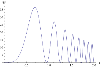
Figure 2: The square of the wave function for the quantum universe. We take the numerical value $\Lambda=1.5$.

4.2 Perfect fluid quantum cosmology

In this case, the Wheeler-DeWitt equation can be constructed by means of the Hamiltonian (39). With the same approximations as we used in the previous subsection, we obtain

$$\left\{\frac{\partial^{2}}{\partial a^{2}}-\left(a^{-1}+6i\Lambda a^{3}\right)\frac{\partial}{\partial a}+\left[\left(36-6i\Lambda\right)a^{2}+12\Lambda a^{4}\right]-ia^{1-3\omega}\frac{\partial}{\partial T}\right\}\Psi(a,T)=0.$$ (77)

We separate the variables in this equation as

$$\Psi(a,T)=e^{iET}\psi(a),$$ (78)

leading to

$$\left\{\frac{d^{2}}{da^{2}}-\left(a^{-1}+6i\Lambda a^{3}\right)\frac{d}{da}+\left[\left(36-6i\Lambda\right)a^{2}+12\Lambda a^{4}+Ea^{1-3\omega}\right]\right\}\psi(a)=0.$$ (79)

The solutions of the above differential equation may be written in the form

$$\psi_{E}(a)=e^{-ia^{2}}\left[c_{1}H_{-\frac{1}{2}-\frac{32+E}{12\Lambda}i}\left(\frac{(1+i)(2+3\Lambda a^{2})}{2\sqrt{3\Lambda}}\right)+c_{2}\,\,\,F_{11}\hskip 11.38092pt\left(\frac{1}{4}+\frac{32+E}{24\Lambda}i,\frac{1}{2};\frac{i(2+3\Lambda a^{2})^{2}}{6\Lambda}\right)\right],$$ (80)

for $\omega=-1/3$ and

$$\psi_{E}(a)=e^{-i(1+\frac{E}{12\Lambda})a^{2}}\left[c_{1}H_{-\frac{1}{2}-\frac{1152\Lambda^{2}-24E\Lambda-E^{2}}{432\Lambda^{3}}i}\left(\frac{(1+i)\left[E+6\Lambda(2+3\Lambda a^{2})\right]}{12\Lambda\sqrt{3\Lambda}}\right)+\right.$$

$$\left.c_{2}\,\,\,F_{11}\hskip 11.38092pt\left(\frac{1}{4}+\frac{1152\Lambda^{2}-24E\Lambda-E^{2}}{864\Lambda^{3}}i,\frac{1}{2};\frac{i\left[E+6\Lambda(2+3\Lambda a^{2})\right]^{2}}{216\Lambda^{3}}\right)\right],$$ (81)

for $\omega=-1$. Now the eigenfunctions of the Wheeler-DeWitt equation can be written as

$$\Psi_{E}(a,T)=e^{iET}\psi_{E}(a).$$ (82)

We may now write the general solution to the Wheeler-DeWitt equation as a superposition of its eigenfunctions; that is,

$$\Psi(a,T)=\int_{0}^{\infty}A(E)\Psi_{E}(a,T)dE,$$ (83)

where $A(E)$ is a suitable weight function to construct the wave packets. The above relations seem to be too complicated to extract an analytical expression for the wave function. Therefore, in the following (for the case $\omega=-1/3$), we present an approximate analytic method which is valid for very small values of scale factor, i.e., in the range that we expect the quantum effects to be important. In this regime if we keep only the $a^{-1}$ and $a^{2}$ terms in the second and third terms of (79), the solutions to this equation can be viewed as a superposition of the functions $\sin\left(\frac{\sqrt{36+E-6i\Lambda}}{2}a^{2}\right)$ and $\cos\left(\frac{\sqrt{36+E-6i\Lambda}}{2}a^{2}\right)$. If we impose the boundary condition $\psi(a=0)=0$ on these solutions, we are led to the following eigenfunctions:

$$\Psi_{E}(a,T)=e^{iET}\sin\left(\frac{\sqrt{36+E-6i\Lambda}}{2}a^{2}\right).$$ (84)

Now, by using the equality

$$\int_{0}^{\infty}e^{-\gamma x}\sin\sqrt{mx}dx=\frac{\sqrt{\pi m}}{2\gamma^{3/2}}e^{-(m/4\gamma)},$$ (85)

we can evaluate the integral over $E$ in (83), and the simple analytical expression for this integral is found if we choose the function $A(E)$ to be a quasi-Gaussian weight factor $A({\cal E})=e^{-\gamma{\cal E}}$ ($\gamma$ is an arbitrary positive constant and ${\cal E}=36+E-6i\Lambda$), which results in

$$\Psi(a,T)=e^{-6(\Lambda+6i)T}\int_{0}^{\infty}e^{-\gamma{\cal E}}e^{i{\cal E}T}\sin\left(\frac{\sqrt{{\cal E}}}{2}a^{2}\right)d{\cal E}.$$ (86)

Using the relation (85) yields the following expression for the wave function

$$\Psi(a,T)={\cal N}e^{-6(\Lambda+6i)T}\frac{a^{2}}{(\gamma-iT)^{3/2}}\exp\left(-\frac{a^{2}}{8(\gamma-iT)}\right),$$ (87)

where ${\cal N}$ is a numerical factor. Now, having this expression for the wave function of the universe, we are going to obtain the predictions for the behavior of the dynamical variables in the corresponding cosmological model. To do this, one may calculate the time dependence of the expectation value of a dynamical variable $q$ as

$$<q>(T)=\frac{<\Psi|q|\Psi>}{<\Psi|\Psi>}.$$ (88)

Following this approach, we may write the expectation value for the scale factor as

$$<a>(T)=\frac{\int_{0}^{\infty}\Psi^{*}(a,T)a\Psi(a,T)da}{\int_{0}^{\infty}\Psi^{*}(a,T)\Psi(a,T)da},$$ (89)

which yields

$$<a>(T)=\sqrt{\frac{\Lambda}{3}}\left(\gamma^{2}+T^{2}\right)^{1/2}.$$ (90)

This relation may be interpreted as the quantum counterpart of the classical solutions (58). However, in spite of the classical solutions, for the wave function (87), the expectation value (90) of $a$ never vanishes, showing that these states are nonsingular. Indeed, in (90) $T$ varies from $-\infty$ to $+\infty$, and any $T_{0}$ is just a specific moment without any particular physical meaning like big-bang singularity. The above result may be written in terms of the cosmic time $\tau$. By the definition $d\tau=a^{-1}(T)dT$, we obtain the quantum version of the relations (63) as

$$<a>(\tau)=\frac{1}{2}\left(e^{\sqrt{\frac{\Lambda}{3}}\tau}+\gamma^{2}e^{-\sqrt{\frac{\Lambda}{3}}\tau}\right).$$ (91)

In figure 3, we have plotted the classical scale factors (58) and (63) and their quantum counterparts (90) and (91). As is clear from this figure, for a perfect fluid with $\omega=-1/3$, the corresponding classical cosmology admits two separate solutions which are disconnected from each other by a classically forbidden region. One of these solutions represents a contracting universe ending in a singularity while another describes an expanding universe which begins its evolution with a big-bang singularity. On the other hand, the evolution of the scale factor based on the quantum-mechanical considerations shows a bouncing behavior in which the universe bounces from a contraction epoch to a reexpansion era. Indeed, the classically forbidden region is where the quantum bounce has occurred. We see that in the late time of cosmic evolution in which the quantum effects are negligible, these two behaviors coincide with each other. This means that the quantum structure which we have constructed has a good correlation with its classical counterpart.

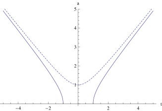
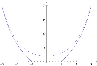
Figure 3: Left: The figure shows qualitative behavior of the classical scale factor (58) (solid lines: the left branch for $a^{(I)}(t)$ and the right branch for $a^{(II)}(t)$) and the expectation value of the scale factor (90) (dashed line). Right: The same figure in terms of cosmic time. The left and right branches of the solid lines represent $a^{(I)}(\tau)$ and $a^{(II)}(\tau)$, respectively, in (63) while the dashed line represents the expectation value (91).

5 Bohmian trajectories

In the previous sections, we saw how the classical singular behavior of the universe was replaced with a bouncing one in a quantum picture. Now, a natural question may arise: Why will the bounce occur? Clearly, it is due to the quantum mechanical effects which show themselves when the size of the universe tends to very small values. However, we would like to know whether the massive correction to the underlying gravity theory has any contribution to this phenomenon. To deal with this question, let us return to the wave function (87) and write it in the polar form $\Psi(a,T)=\Omega(a,T)e^{iS(a,T)}$, where $\Omega(a,T)$ and $S(a,T)$ are real functions, which simple algebra gives as

$$\Omega(a,T)=e^{-6\Lambda T}\frac{a^{2}}{(\gamma^{2}+T^{2})^{3/4}}\exp\left[-\frac{\gamma a^{2}}{8(\gamma^{2}+T^{2})}\right],$$ (92)

$$S(a,T)=-36T+\frac{3}{2}\arctan\frac{T}{\gamma}-\frac{Ta^{2}}{8(\gamma^{2}+T^{2})}.$$ (93)

According to the Bohm-de Broglie interpretation of quantum mechanics [23] and also its usage in quantum cosmology [24], upon using this form of the wave function in the corresponding wave equation, we arrive at the modified Hamilton-Jacobi equation as

$${\cal H}\left(q_{i},P_{i}=\frac{\partial S}{\partial q_{i}}\right)+{\cal Q}=0,$$ (94)

where $P_{i}$ are the momentum conjugate to the dynamical variables $q_{i}$ and ${\cal Q}$ is the quantum potential. With beginning of the wave equation (77), for which we have used the same approximations as in the previous section, the above mentioned procedure gives the quantum potential as

$${\cal Q}=\frac{1}{\Omega}\frac{\partial^{2}\Omega}{\partial a^{2}}-\frac{1}{a\Omega}\frac{\partial\Omega}{\partial a}.$$ (95)

On the other hand, the Bohmian equations of motion can be obtained by $P_{a}=\frac{\partial S}{\partial a}$, where by means of the relation (34) reads

$$-6a\dot{a}+3\Lambda a^{2}=-\frac{T}{4(\gamma^{2}+T^{2})}.$$ (96)

The solution to this equation denotes the Bohmian representation of the scale factor; that is

$$a(t)=\sqrt{ce^{\Lambda T}+\frac{1}{24}e^{\Lambda T-i\gamma\Lambda}\left[e^{2i\gamma\Lambda}\mbox{ Ei}(1;-\Lambda T-i\gamma\Lambda)+\mbox{Ei}(1;-\Lambda T+i\gamma\Lambda)\right]},$$ (97)

where $c$ is an integration constant and $\mbox{Ei}(b;z)$ is the exponential integral function defined by

$$\mbox{Ei}(b;z)=\int_{1}^{\infty}e^{-kz}k^{-b}dk.$$ (98)

The bouncing behavior of the scale factor is again its main property near the classical singularities as we have shown in figure 4. To achieve an expression for the quantum potential in terms of the scale factor, we note that all of our above calculations are in the vicinity of $T\sim 0$, where the scale factor is small. In this regime, a numerical analysis shows that the Bohmian scale factor (97) behaves as $a(T)\sim(\gamma^{2}+T^{2})^{1/2}$, in agreement with the expectation value (90). Thus, substituting in (92), we get the quantum potential from (95) as

$${\cal Q}(a)=\frac{3}{4}\left[\gamma^{2}\left(\frac{1}{a^{4}-\gamma^{2}a^{2}}+\frac{8\Lambda}{(a^{2}-\gamma^{2})^{3/2}}\right)+\frac{-1+48\Lambda^{2}a^{2}}{a^{2}-\gamma^{2}}\right].$$ (99)

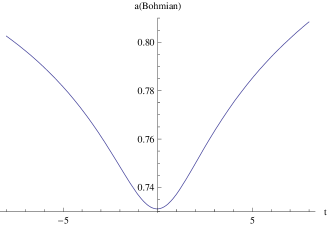
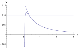
Figure 4: Left: The Bohmian trajectory of the scale factor. Right: The horizontal line represents a typical energy level. The solid curve is the quantum potential for $\Lambda\neq 0$, while the dashed curve denotes the quantum potential when $\Lambda=0$.

In figure 4 we also have plotted the qualitative behavior of the quantum potential versus the scale factor. As this figure shows, this potential goes to zero for the large values of the scale factor. This behavior is expected, since in this regime the quantum effects can be neglected and the universe evolves classically. On the other hand, for the small values of the scale factor the potential takes a large magnitude and the quantum mechanical considerations come into the scenario. This is where the quantum potential can produce a huge repulsive force which may be interpreted as being responsible of the avoidance of singularity. In figure 4 the horizontal line represents a constant energy level which in intersecting with the potential curves gives the turning points at which the bounce will occur. The solid curve in this figure is plotted in the case of $\Lambda\neq 0$; i.e., for the massive theory, while the dashed curve is for $\Lambda=0$; i.e., for when the massive corrections are absent. It is seen that, although the mass term $\Lambda$ is not the only reason for the bouncing behavior in the vicinity of the classical singularity, it may shift the bouncing point into the smaller values of the scale factor. This means that if we consider the bouncing point as the minimum size of the universe (which is suggested by quantum cosmology), then the massive version of the underlying gravity theory predicts a smaller value for this minimal size in comparison with the usual Einstein-Hilbert model. These facts and also other considerable possibilities such as quantum tunneling between different classically allowed regimes (as can be seen from figure 4) through the potential barrier support the idea that the massive corrections to the classical cosmology are some signals from quantum gravity.

6 Conclusions

In this paper we have applied the recently proposed nonlinear massive theory of gravity to an open FRW cosmological setting. Although the absence of homogeneous and isotropic solutions is one of the main challenges related to this kind of gravitational theory, we moved along the lines of [6, 7], in which the existence of open FRW cosmologies is investigated. By using the constraint corresponding to the Stückelberg scalars, we reduced the number of degrees of freedom, according to which the total Hamiltonian of the model is deduced. We then presented in detail, the classical cosmological solutions either for the empty universe or in the case where the universe is filled by a perfect fluid (in its Schutz representation) with the equation of state parameter $\omega=-1/3,-1$. We saw that in both of these cases, the solutions consist of a contraction universe which finalizes its evolution in a singular point and an expanding universe which begins its dynamic with a big-bang singularity. These two branches of solutions are disconnected from each other by a classically forbidden region. Also, the common feature of the vacuum and matter classical solutions is that the mass term plays a role which resembles the role of cosmological constant in the usual de Sitter universe. In this sense we may relate the massive corrections of GR to the problem of dark energy.

In another part of the paper, we dealt with the quantization of the model described above via the method of canonical quantization. For an empty universe, we have shown that by applying the WKB approximation on the Wheeler-DeWitt equation, one can recover the late time behavior of the classical solutions. For the early universe, we obtained oscillatory quantum states free of classical singularities by which two branches of classical solutions may communicate with each other. In the presence of matter, we focused our attention on the approximate analytical solutions to the Wheeler-DeWitt equation in the domain of small scale factor, i.e. in the region which the quantum cosmology is expected to be dominant. Using Schutz s representation for the perfect fluid, under a particular gauge choice, we led to the identification of a time parameter which allowed us to study the time evolution of the resulting wave function. Investigation of the expectation value of the scale factor shows a bouncing behavior near the classical singularity. In addition to singularity avoidance, the appearance of bounce in the quantum model is also interesting in its nature due to prediction of a minimal size for the corresponding universe. We know the idea of existence of a minimal length in nature is supported by almost all candidates of quantum gravity. Finally, we repeated the quantum calculations by means of the Bohmian approach to quantum mechanics. The analysis of the quantum potential shows the importance of the mass term in the action of the model. Indeed, we have shown that in the presence of the massive graviton, the quantum potential changes its behavior from an infinite barrier to a finite one, and hence the minimal size of the universe, from which the bounce occurs, will be shifted to the smaller values. Also, the massive theory of quantum cosmology exhibits some other possibilities; for example, tunneling between different classically allowed regions, for cosmic evolution in the early universe epoch.

References

- [1] M. Fierz and W. Pauli, Proc. R. Soc. A 173 (1939) 211
- [2] D.G. Boulware and S. Deser, Phys. Rev. D 6 (1972) 3368
- [3] C. de Rham and G. Gabadadze, Phys. Rev. D 82 (2010) 4 (arXiv: 1007.0443 [hep-th])
-
[4]
K. Koyama, G. Niz and G. Tasinato, Phys. Rev. Lett. 107 (2011) 131101 (arXiv: 1103.4708
[hep-th])
K. Koyama, G. Niz and G. Tasinato, Phys. Rev. D 84 (2011) 064033 (arXiv: 1104.2143 [hep-th])
T.M. Nieuwenhuizen, Phys. Rev. D 84 (2011) 024038 (arXiv: 1103.5912 [gr-qc])
S.F. Hassan and R.A. Rosen, Phys. Rev. Lett. 108 (2012) 041101 (arXiv: 1106.3344 [hep-th])
C. de Rham, G. Gabadadze and A.J. Tolley, Phys. Lett. B 711 (2012) 190 (arXiv: 1107.3820 [hep-th])
C. de Rham, G. Gabadadze and A.J. Tolley, Helicity Decomposition of Ghost-free Massive Gravity, (arXiv: 1108.4521 [hep-th])
L. Berezhiani, G. Chkareuli, C. de Rham, G. Gabadadze, A.J. Tolley, On Black Holes in Massive Gravity (arXiv: 1111.3613 [hep-th]) - [5] G. D’Amico, C. de Rham, S. Dubovsky, G. Gabadadze, D. Pirtskhalava and A.J. Tolley, Phys. Rev. D 84 (2011) 124046 (2011) (arXiv: 1108.5231 [hep-th])
- [6] A.E. Gümrükçüoğlu, C. Lin and S. Mukohyama, J. Cosmol. Astropart. Phys. 11 (2011) 030 (arXiv: 1109.3845 [hep-th])
- [7] A.E. Gümrükçüoğlu, C. Lin and S. Mukohyama, J. Cosmol. Astropart. Phys. 03 (2012) 006 (arXiv: 1111.4107 [hep-th])
-
[8]
M.S. Volkov, J. High Energy Phys. 01 (2012) 035 (arXiv: 1110.6153
[hep-th]),
D. Comelli, M. Crisostomi, F. Nesti and L. Pilo, J. High Energy Phys. 03 (2012) 065 (arXiv: 1111.1983 [hep-th])
M. von Strauss, A. Schmidt-May, J. Enander, E. Mortsell and S.F. Hassan, Cosmological Solutions in Bimetric Gravity and Their Observational Tests, (arXiv: 1111.1655 [gr-qc])
N. Khosravi, N. Rahmanpour, H.R. Sepangi and S. Shahidi, Phys. Rev. D 85 (2012) 024049 (arXiv: 1111.5346 [hep-th])
N. Khosravi, H.R. Sepangi and S. Shahidi, On massive cosmological scalar perturbations, (arXiv: 1202.2767 [gr-qc]) -
[9]
S.F. Hassan and R.A. Rosen, J. High Energy Phys. 01 (2012) 126 (arXiv: 1109.3515 [hep-th])
S.F. Hassan and R.A. Rosen, Confirmation of the Secondary Constraint and Absence of Ghost in Massive Gravity and Bimetric Gravity, (arXiv: 1111.2070 [hep-th])
S.F. Hassan and R.A. Rosen, On Non-Linear Actions for Massive Gravity, (arXiv: 1103.6055 [hep-th]) - [10] C. de Rham, G. Gabadadze and A.J. Tolley, Phys. Rev. Lett. 106 (2011) 231101 (arXiv: 1011.1232 [hep-th])
-
[11]
N. Arkani-Hamed, H. Georgi and M.D. Schwartz, Ann. Phys. 305 (2003) 96 (arXiv: hep-th/0210184)
S.L. Dubovsky, J. High Energy Phys. 10 (2004) 076 (arXiv: hep-th/0409124) -
[12]
B.F. Schutz, Phys. Rev. D 2 (1970)
2762
B.F. Schutz, Phys. Rev. D 4 (1971) 3559
V.G. Lapchinskii, V.A. Rubakov, Theor. Math. Phys. 33 (1977) 1076 -
[13]
A.B. Batista, J.C. Fabris, S.V.B. Goncalves and J. Tossa, Phys. Lett. A 283 (2001) 62
(arXiv: gr-qc/0011102)
F.G. Alvarenga, J.C. Fabris, N.A. Lemos and G.A. Monerat, Gen. Rel. Grav. 34 (2002) 651 (arXiv: gr-qc/0106051)
A.B. Batista, J.C. Fabris, S.V.B. Goncalves and J. Tossa, Phys. Rev. D 65 (2002) 063519 (arXiv: gr-qc/0108053)
B. Vakili, Phys. Lett. B 688 (2010) 129 (arXiv: 1004.0306 [gr-qc])
B. Vakili, Class. Quantum Grav. 27 (2010) 025008 (arXiv: 0908.0998 [gr-qc]) - [14] Ø. Grøn and S. Hervik, Einstein’s General Theory of Relativity (Springer, New York, 2007)
- [15] A. Anderson, Ann. Phys. 232 (1994) 292 (arXiv: hep-th/9305054)
- [16] S.W. Hawking and D.N. Page, Nucl. Phys. B 264 (1986) 185
- [17] R. Steigl and F. Hinterleitner, Class. Quantum Grav. 23 (2006) 3879
-
[18]
A. Vilenkin, Phys. Rev. D 37 (1988) 888
A. Vilenkin, Phys. Rev. D 33 (1986) 3560 - [19] N.A. Lemos, J. Math. Phys. 37 (1996) 1449 (arXiv: gr-qc/9511082)
- [20] B.S. DeWitt, Phys. Rev. 160 (1967) 1113
- [21] C. Kiefer, Quantum Gravity (Oxford University Press, New York, 2007).
-
[22]
D.H. Coule and J. Martin, Phys. Rev. D 61 (2000) 063501 (arXiv: gr-qc/9905056)
A. Linde, J. Cosmol. Astropart. Phys. 10 (2004) 004 (arXiv: hep-th/0408164) -
[23]
D. Bohm, Phys. Rev. 85 (1952) 166
D. Bohm, Phys. Rev. 85 (1952) 180
P.R. Holland, The Quantum Theory of Motion: An Account of the de Broglie-Bohm Interpretation of Quantum Mechanics, (Cambridge University Press, Cambridge, 1993) -
[24]
F.T. Falciano and N. Pinto-Neto, Phys. Rev. D 79 (2009) 023507 (arXiv:
0810.3542 [gr-qc])
A. Shojai and F. Shojai, Europhys. Lett. 71 (2005) 886 (arXiv: gr-qc/0409020)