Isospin violating decay of $\psi(3770)\rightarrow J/\psi+\pi^{0}$

Abstract

The strong-isospin violation in $\psi(3770)\rightarrow J/\psi+\pi^{0}$ via intermediate $D$ meson loops is investigated in an effective Lagrangian approach. In this process, there is only one $D$-meson loop contributing to the absorptive part, and the uncertainties due to the introduction of form factors can be minimized. With the help of QCD spectral sum rules (QSSR), we extract the $J/\psi DD^{*}$ form factor as an implement from the first principle of QCD. The $DD^{*}\pi^{0}$ form factor can be well determined from the experimental data for $D\rightarrow\pi l\nu$. The exploration of the dispersion relation suggests the dominance of the dispersive part via the intermediate $D$ meson loops even below the open charm threshold. This investigation could provide further insights into the puzzling question on the mechanisms for $\psi(3770)\to$ non-$D\bar{D}$ transitions.

I Introduction

The non-$D\bar{D}$ decays of $\psi(3770)$ have attracted a lot attention during the past decades. As $\psi(3770)$ is the first state above the open charm $D\bar{D}$ threshold, its decay was believed to be saturated by the $D\bar{D}$ channel via the Okubo-Zweig-Iizuka (OZI) connected diagram. Such an anticipation was supported by early experimental data which showed that exclusive decays of $\psi(3770)\to$ non-$D\bar{D}$ were negligibly small. Theoretical calculations of the perturbative QCD (pQCD) leading order contributions also suggested rather small non-$D\bar{D}$ branching ratios for $\psi(3770)$ Kuang:1989ub ; Ding:1991vu ; Rosner:2001nm ; Rosner:2004wy ; Eichten:2007qx ; Voloshin:2005sd .

Interestingly, recent studies of the $\psi(3770)$ non-$D\bar{D}$ decays in experiment and theory have exposed unexpected results which complicated the situation. In experiment, the $D\bar{D}$ cross section measurement by the CLEO collaboration suggests that the non-$D\bar{D}$ branching ratio is consistent with zero with an upper limit of about 6.8% He:2005bs ; :2007zt ; Besson:2005hm . Rather contradicting the CLEO results, the BES collaboration finds much larger non-$D\bar{D}$ branching ratios of $\sim 15\%$ in the direct measurement of non-$D\bar{D}$ inclusive cross section bes-3770 . Recently a next-to-leading-order (NLO) nonrelativistic QCD (NRQCD) calculation of the $c\bar{c}$ annihilation width for $\psi(3770)$ suggests that the higher order contributions can account for about $5\%$ of the $\psi(3770)$ non-$D\bar{D}$ decay branching ratios at most He:2008xb . In Refs. Zhang:2009kr ; Liu:2009dr , it was proposed that the open-charm threshold effects via intermediate meson loops (IML) could serve as an important nonperturbative mechanism to produce sizable non-$D\bar{D}$ branching ratios. Note that $\psi(3770)$ is close to the $D\bar{D}$ open threshold. A natural conjecture is that the $D\bar{D}$ threshold would play an important role in its production and decay. This mechanism turns out to be successful in the explanation of the decay of $\psi(3770)\to\text{vector}+\text{pseudoscalar}$ as one of the non-$D\bar{D}$ decay channel of $\psi(3770)$ Zhang:2009kr ; Liu:2009dr .

During the past few years, there have been observations of a large number of heavy quarkonium states Olsen:2009ys at the B-factories (Belle and BaBar) and electron storage-rings (CLEO). Some of those states have masses close to open thresholds and cannot be easily accommodated in the framework of potential quark models. For instance, the well-established $X(3872)$ is located in the vicinity of $D^{*}\bar{D}$ threshold and its mass as a $1^{++}$ state is nearly 100 MeV lower than the first radial excitation of $\chi_{c1}$ in potential models. Such observations, on the one hand, have raised serious questions on the constituent degrees of freedom within heavy quarkonia, and on the other hand, raised questions on the role played by the open decay thresholds via the IML as an important nonperturbative mechanism in the understanding of the properties of those newly observed states. Such a mechanism symbolizes a general dynamical feature in the charmonium mass region, thus should be explored broadly in various processes.

To gain further insights into the underlying dynamics and understand better the properties of the IML, we are motivated to study the decays of $\psi(3770)\to J/\psi+\eta$ and $J/\psi+\pi^{0}$. First, we note that the decay of $\psi(3770)\to J/\psi+\eta$ is one of few measured non-$D\bar{D}$ decay channels in experiment with $BR(\psi(3770)\to J/\psi+\eta)=(9\pm 4)\times 10^{-4}$ Nakamura:2010zzi . One can estimate the branching ratio of $\psi(3770)\to J/\psi+\pi^{0}$ via $\eta$-$\pi^{0}$ mixing based on the leading-order chiral perturbation theory. The mixing intensity can be expressed as Gross:1979ur

$$\epsilon_{0}=\frac{\sqrt{3}}{4}\frac{m_{d}-m_{u}}{m_{s}-(m_{u}+m_{d})/2}.$$ (1)

Using Dashen’s theorem Dashen:1969eg , one obtains

$$\epsilon_{0}=\frac{1}{\sqrt{3}}\frac{M_{K^{0}}^{2}-M_{K^{+}}^{2}+M_{\pi^{+}}^{2}-M_{\pi^{0}}^{2}}{M_{\eta}^{2}-M_{\pi^{0}}^{2}}=0.01\ .$$ (2)

Taking the $\eta-\eta^{\prime}$ mixing into account, the mixing intensity is slightly enhanced Kroll:2005sd

$$\hat{\epsilon}=\epsilon_{0}\sqrt{3}\cos\phi,$$ (3)

where $\sqrt{3}\cos\phi=1.34$ would be unity if $\phi$ is the ideal mixing angle. With the $\eta$-$\pi^{0}$ mixing intensity in a range of $0.01\sim 0.02$, the branching ratio of $\psi(3770)\to J/\psi+\pi^{0}$ from $\eta$-$\pi^{0}$ mixing is at most the order of $10^{-6}$. This result actually sets up a limit for the $\eta$-$\pi^{0}$ mixing contributions in $\psi(3770)\to J/\psi+\pi^{0}$. In contrast, the Particle Data Group (PDG2010) Nakamura:2010zzi gives an experimental upper limit $BR(\psi(3770)\to J/\psi+\pi^{0})<2.8\times 10^{-4}$. A recent investigation of $\psi^{\prime}\to J/\psi+\pi^{0}$ Guo:2009wr ; Guo:2010ak based on a nonrelativistic effective field theory (NREFT) suggests that the strong-isospin violation via the IML is relatively enhanced by $1/v$ in comparison with the tree-level contribution where the pion is emitted directly from the charmonium through soft gluon exchanges, where $v\simeq 0.5$ is the velocity of the intermediate charmed meson. Since $\psi(3770)$ is close to the $D\bar{D}$ threshold, we expect that such a strong-isospin mechanism would also play a role. As a consequence, the IML mechanism may lead to a sizable branching ratio of $\psi(3770)\to J/\psi+\pi^{0}$ which might be significantly larger than that given by the $\eta$-$\pi^{0}$ mixing. In an early study Achasov:1990gt ; Achasov:1994vh ; Achasov:2005qb , the absorptive contribution from the intermediate $D\bar{D}$ in the decay of $\psi(3770)\to J/\psi+\pi^{0}(\eta)$ was calculated with an exponential form factor determined by the characteristic mass scale in the exchange channel. It was also argued that the real part contribution from $D\bar{D}$ and other heavier $D$ meson loops should cancel each other in order to obey the OZI rule successfully in $J/\psi$ decay. However, it is found Wang:2012mf that the IML effects may still be important in the decay of charmonium close to the open charm threshold. This is because the quark-hadron duality turns out to have been broken locally. As a consequence, the decay of a charmonium state can still experience the open threshold effects significantly if its mass is close to the open threshold. Such a scenario may imply that the real parts of the exclusive $\psi(3770)$ decays could not be neglected and could explain the observed sizeable non-$D\bar{D}$ branching ratios of $\psi(3770)$ bes-3770 .

In this work, we shall apply an effective Lagrangian approach (ELA) to investigate the IML effects in $\psi(3770)\to J/\psi+\pi^{0}$, and demonstrate that the IML transitions have dominant contributions to this isospin-violating decay channel. As an important improvement of this approach, we shall implement form factors from QCD spectral sum rules (QSSR) for the off-shell $J/\psi DD^{*}$ coupling vertex, while the $D^{*}D\pi^{0}$ form factor can be extracted from the semileptonic decay of $D\to\pi^{0}l\nu$. We mention in advance that this elaborate treatment will allow a reliable estimate of the absorptive amplitude of $\psi(3770)\to J/\psi+\pi^{0}$. Meanwhile, we also explore the real part of the IML contributions with the help of dispersion relation, within which the effective threshold is determined by the experimental data of $\psi(3770)\to J/\psi+\eta$.

This paper is organized as follows: In Sec. II the ELA for the IML transitions is formulated. In Sec. III the form factors from QCDSR and $D$ meson semileptonic decays are investigated. The numerical results for the isospin-violating decay $\psi(3770)\to J/\psi+\pi^{0}$ are presented in Sec. IV, and a brief summary is given in Sec. V.

II Isospin-violating decay of $\psi(3770)\rightarrow J/\psi+\pi^{0}$ via IML transitions

II.1 Absorptive part

As illustrated by Fig. 1, only the $DD(D^{*})$ loop (the meson in the parenthesis denotes the exchanged particle between $J/\psi$ and $\pi^{0}$) contributes to the imaginary part. The effective Lagrangians are as follows Colangelo:2003sa ; Casalbuoni:1996pg ,

$$\mathcal{L}_{\psi^{\prime\prime}DD} = -ig_{\psi^{\prime\prime}DD}\psi^{\prime\prime\mu}D_{i}^{\dagger}\stackrel{{\scriptstyle\leftrightarrow}}{{\partial_{\mu}}}D_{i}\ ,$$ (4)

$$\mathcal{L}_{\psi DD^{*}} = g_{\psi DD^{*}}\epsilon_{\mu\nu\alpha\beta}\partial^{\mu}\psi_{n}^{\nu}\{D_{i}^{*\beta{\dagger}}\stackrel{{\scriptstyle\leftrightarrow}}{{\partial^{\alpha}}}D_{i}-D_{i}^{\dagger}\stackrel{{\scriptstyle\leftrightarrow}}{{\partial^{\alpha}}}D_{i}^{*\beta}\}\ ,$$ (5)

$$\mathcal{L}_{D^{*}D\pi} = -ig_{D^{*}DP}\left(D^{i}\partial^{\mu}P_{ij}D_{\mu}^{*j{\dagger}}-D_{\mu}^{*i}\partial^{\mu}P_{ij}D^{j{\dagger}}\right)\ ,$$ (6)

where the coupling $g_{\psi DD^{*}}\equiv M_{\psi}/(f_{\psi}\sqrt{M_{D^{*}}M_{D}})\ \mathrm{GeV}^{-1}$. The same convention has also been adopted in Ref. Wang:2012mf .

The decay amplitude via the $D\bar{D}(D^{*})$ loop is

$$\mathcal{M}_{fi} = \sum_{Polarization}\int\frac{\mathrm{d}^{4}p_{5}}{(2\pi)^{4}}(2g_{\psi^{\prime\prime}DD}p_{3}\cdot\epsilon_{1})(-2g_{\psi DD^{*}}\epsilon_{\mu\nu\alpha\beta}q_{2}^{\mu}\epsilon_{2}^{*\nu}p_{5}^{\alpha}\epsilon_{5}^{\beta})(\frac{-g_{D^{*}DP}}{\sqrt{2}}p\cdot\epsilon_{5}^{*})$$ (7)

$$\times\frac{i}{p_{3}^{2}-M_{D}^{2}}\frac{i}{p_{4}^{2}-M_{D}^{2}}\frac{i}{p_{5}^{2}-M_{D^{*}}^{2}}F(p_{i}^{2})\ .$$

At each vertex of the loop diagram, the off-shell effect or the finite size effect should be taken into account by introducing the form factor $F(p_{i}^{2})$, which can be regarded as the extended version of the local couplings in the original effective Lagrangian. The form factor is also necessary for cutting off the ultraviolet divergence in the loop integrals.

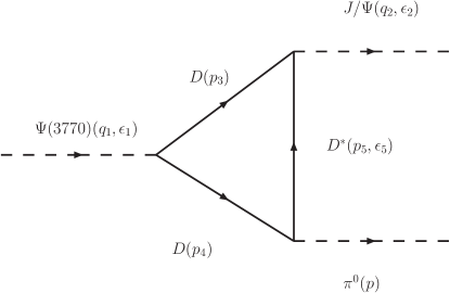
Figure 1: The $D$-loop diagram contributing to the absorptive part.

Applying the Cutkosky rule, the discontinuity of the decay amplitude is

$$\emph{Disc.}\mathcal{M}_{fi} = -i(-2\pi i)^{2}\int\frac{\mathrm{d}^{4}p_{5}}{(2\pi)^{4}}(2g_{\psi^{\prime\prime}DD})(p_{3}\cdot\epsilon_{1})\epsilon_{q_{2}\epsilon_{2}^{*}p_{5}\mu}p_{\nu}\left(-g^{\mu\nu}+\frac{p_{5}^{\mu}p_{5}^{\nu}}{M_{D^{*}}^{2}}\right)$$ (8)

$$\times\delta(p_{3}^{2}-M_{D}^{2})\times\delta(p_{4}^{2}-M_{D}^{2})\times\frac{F_{\psi DD^{*}}(p_{5}^{2})F_{D^{*}D\pi^{0}}(p_{5}^{2})}{p_{5}^{2}-M_{D^{*}}^{2}}$$

with $\epsilon_{q_{2}\epsilon_{2}^{*}p_{5}\mu}\equiv\epsilon_{\alpha\beta\gamma\mu}q_{2}^{\alpha}\epsilon_{2}^{*\beta}p_{5}^{\gamma}$ for a short notation. Then, there are two form factors depending only on the virtuality of $D^{*}$ left in our calculation. In practice, the product of these form factors can be parameterized as the product of the local couplings and an empirical form factor:

$$F_{\psi_{n}DD^{*}}(p_{5}^{2})F_{D^{*}D\pi^{0}}(p_{5}^{2})\equiv-2g_{\psi_{n}DD^{*}}\frac{-g_{D^{*}DP}}{\sqrt{2}}F(p_{5}^{2})\ ,$$ (9)

where a dipole form factor is adopted,

$$F(p_{5}^{2})=\left(\frac{\Lambda^{2}-M_{D^{*}}^{2}}{\Lambda^{2}-p_{5}^{2}}\right)^{2},$$ (10)

with $\Lambda=M_{D^{*}}+\alpha\Lambda_{QCD}$ and $\Lambda_{QCD}=0.22\ \mathrm{GeV}$.

Further deduction gives the discontinuity of the decay amplitude

$$\emph{Disc.}\mathcal{M}_{fi} = 2ig_{\psi^{\prime\prime}DD}\int\frac{\mathrm{d}^{3}\vec{p}_{3}}{(2\pi)^{3}2E_{p_{3}}2E_{p_{4}}}\frac{F_{\psi DD^{*}}(p_{5}^{2})F_{D^{*}D\pi^{0}}(p_{5}^{2})}{p_{5}^{2}-M_{D^{*}}^{2}}$$ (11)

$$\times 2\pi\delta(p_{3}^{0}+p_{4}^{0}-q_{1}^{0})\epsilon_{q_{2}\epsilon_{2}^{*}p_{3}p}p_{3}\cdot\epsilon_{1}|_{constraints}\ ,$$

where $E_{p_{i}}=\sqrt{|\vec{p}_{i}|^{2}+M_{i}^{2}}$, and $constraints\equiv(p_{3}^{0}>0,p_{4}^{0}>0,p_{3}^{2}=M_{D}^{2},p_{4}^{2}=M_{D}^{2},p_{5}=q_{2}-p_{3},\vec{p}_{4}=\vec{p}_{5}+\vec{p})$.

Extracting the antisymmetric Lorentz structure $\epsilon_{q_{2}\epsilon_{2}^{*}\mu p}\epsilon_{1\nu}$, we get the tensor amplitude

$$\emph{Disc.}\mathcal{M}_{fi}^{\mu\nu} = 2ig_{\psi^{\prime\prime}DD}\int\frac{\mathrm{d}^{3}\vec{p}_{3}}{(2\pi)^{3}2E_{p_{3}}2E_{p_{4}}}\frac{F_{\psi DD^{*}}(p_{5}^{2})F_{D^{*}D\pi^{0}}(p_{5}^{2})}{p_{5}^{2}-M_{D^{*}}^{2}}$$ (12)

$$\times 2\pi\delta(p_{3}^{0}+p_{4}^{0}-q_{1}^{0})p_{3}^{\mu}p_{3}^{\nu}|_{constraints}$$

From Lorentz invariance, this tensor structure can be decomposed into terms built out of the external momenta and metric tensor:

$$\emph{Disc.}\mathcal{M}_{fi}^{\mu\nu} = g^{\mu\nu}\mathcal{M}_{A}+p^{\mu}p^{\nu}\mathcal{M}_{B}+q_{2}^{\mu}q_{2}^{\nu}\mathcal{M}_{C}+(p^{\mu}q_{2}^{\nu}+p^{\nu}q_{2}^{\mu})\mathcal{M}_{D},$$ (13)

where only $\mathcal{M}_{A}$ will contribute to the final result when we contract the tensor amplitude with the extracted antisymmetric Lorentz structure.

Contracting the tensor amplitude with the metric tensor, we obtain

$$g_{\mu\nu}\emph{Disc.}\mathcal{M}_{fi}^{\mu\nu} = 2ig_{\psi^{\prime\prime}DD}\int\frac{\mathrm{d}^{3}\vec{p}_{3}}{(2\pi)^{3}2E_{p_{3}}2E_{p_{4}}}\frac{F_{\psi DD^{*}}(p_{5}^{2})F_{D^{*}D\pi^{0}}(p_{5}^{2})}{p_{5}^{2}-M_{D^{*}}^{2}}$$

$$\times 2\pi\delta(p_{3}^{0}+p_{4}^{0}-q_{1}^{0})p_{3}^{2}|_{constraints}$$

$$= 2ig_{\psi^{\prime\prime}DD}\int\frac{|\vec{p}_{3}|^{2}\mathrm{d}|\vec{p}_{3}|\sin\theta\mathrm{d}\theta\mathrm{d}\varphi}{(2\pi)^{3}2E_{p_{3}}2E_{p_{4}}}\frac{F_{\psi DD^{*}}(p_{5}^{2})F_{D^{*}D\pi^{0}}(p_{5}^{2})}{p_{5}^{2}-M_{D^{*}}^{2}}$$

$$\times 2\pi\delta(p_{3}^{0}+p_{4}^{0}-q_{1}^{0})p_{3}^{2}|_{constraints}$$

In the rest frame of $\psi(3770)$ and setting the direction of $\vec{q}_{2}$ as the $z$-axis, the dynamic variables can be expressed as

$$h \equiv |\vec{q}_{2}|=\sqrt{\left(\frac{M_{\psi}^{2}+M_{\psi^{\prime\prime}}^{2}-M_{\pi}^{2}}{2M_{\psi^{\prime\prime}}}\right)^{2}-M_{\psi}^{2}}$$

$$\frac{r}{2} \equiv |\vec{p}_{3}|=\frac{\sqrt{M_{\psi^{\prime\prime}}^{2}-4M_{D}^{2}}}{2}$$

$$v \equiv q_{2}^{0}=\frac{M_{\psi^{\prime\prime}}^{2}+M_{\psi}^{2}-M_{\pi}^{2}}{2M_{\psi^{\prime\prime}}}$$

$$w \equiv p^{0}=\frac{M_{\psi^{\prime\prime}}^{2}-M_{\psi}^{2}+M_{\pi}^{2}}{2M_{\psi^{\prime\prime}}}$$

$$q_{1}^{0} = v+w=M_{\psi^{\prime\prime}}$$

$$p_{3}^{0} = \frac{v+w}{2}$$ (15)

Then, the Lorentz invariant amplitude is

$$g_{\mu\nu}\emph{Disc.}\mathcal{M}_{fi}^{\mu\nu} = ig_{\psi^{\prime\prime}DD}\times\frac{r}{8\pi(v+w)}\times\int_{-1}^{1}\mathrm{d}x\,\frac{M_{D}^{2}F_{\psi DD^{*}}(x)F_{D^{*}D\pi^{0}}(x)}{G(x)}$$

where the propagator of $D^{*}$ is $G(x)=M_{\psi}^{2}+M_{D}^{2}-2[v(v+w)/2-hrx/2]-M_{D^{*}}^{2}$.

Similarly, we can get other three Lorentz invariant amplitudes:

$$p_{\mu}p_{\nu}\emph{Disc.}\mathcal{M}_{fi}^{\mu\nu} = ig_{\psi^{\prime\prime}DD}\times\frac{r}{8\pi(v+w)}$$

$$\times\int_{-1}^{1}\mathrm{d}x\,\frac{[w(v+w)/2+hrx/2]^{2}F_{\psi DD^{*}}(x)F_{D^{*}D\pi^{0}}(x)}{G(x)}$$

$$q_{2\mu}q_{2\nu}\emph{Disc.}\mathcal{M}_{fi}^{\mu\nu} = ig_{\psi^{\prime\prime}DD}\times\frac{r}{8\pi(v+w)}$$

$$\times\int_{-1}^{1}\mathrm{d}x\,\frac{[v(v+w)/2-hrx/2]^{2}F_{\psi DD^{*}}(x)F_{D^{*}D\pi^{0}}(x)}{G(x)}$$

$$p_{\mu}q_{2\nu}\emph{Disc.}\mathcal{M}_{fi}^{\mu\nu} = ig_{\psi^{\prime\prime}DD}\times\frac{r}{8\pi(v+w)}$$

$$\times\int_{-1}^{1}\mathrm{d}x\,\frac{[v(v+w)/2-hrx/2][w(v+w)/2+hrx/2]F_{\psi DD^{*}}(x)F_{D^{*}D\pi^{0}}(x)}{G(x)}$$

Solving these four equations simultaneously, we can get the complicated expression of the invariant amplitude $\mathcal{M}_{A}$ and the absorptive part of the decay amplitude $\emph{Disc.}\mathcal{M}_{fi}$. The charge conjugate contribution gives the same result.

Because of the mass of $\psi(3770)$ being above the charmed meson pair, the coupling constant $g_{\psi^{\prime\prime}DD}$ and the isospin difference may be difficult to get from theory because of the rescattering mechanism. So we will extract this coupling directly from the experimental data:

$$\Gamma_{\psi^{\prime\prime}\rightarrow D\bar{D}} = \frac{4g_{\psi^{\prime\prime}DD}^{2}|\vec{p}_{3}|}{8\pi M_{\psi^{\prime\prime}}^{2}}\times\frac{1}{3}\sum_{\epsilon_{1}}(p_{3}\cdot\epsilon_{1})(p_{3}\cdot\epsilon_{1}^{*})$$ (20)

$$= \frac{g_{\psi^{\prime\prime}DD}^{2}|\vec{p}_{3}|}{6\pi M_{\psi^{\prime\prime}}^{2}}\left(-M_{D}^{2}+\frac{M_{\psi^{\prime\prime}}^{2}}{4}\right)\ .$$

II.2 Dispersive part

In principle, all the meson loops of which the thresholds are above the $\psi(3770)$ mass would contribute to the dispersive part (i.e. the real part) of the transition amplitude. Because of the introduction of form factors in the loop integrals, some model dependence seems inevitable in the evaluation of the real part. Given that the imaginary part of the amplitude can be reliably determined as in the previous subsection, we shall apply the dispersion relation to obtain the real part of the decay amplitude. Taking the assumption that the spectral density can be approximated by the extrapolation $\mathcal{M}_{A}(M_{\psi^{\prime\prime}}^{2})\rightarrow\mathcal{M}_{A}(s_{1})$, we have the unsubtracted dispersion relation:

$$Re[\mathcal{M}_{fi}^{Tot}]=\frac{1}{2\pi i}\left(\mathcal{P}\int_{(2M_{D^{+}})^{2}}^{{th_{C}}}\frac{2\mathcal{M}_{A}^{C}(s_{1})}{s_{1}-M_{\psi^{\prime\prime}}^{2}}\mathrm{d}s_{1}+\mathcal{P}\int_{(2M_{D^{0}})^{2}}^{{th_{N}}}\frac{2\mathcal{M}_{A}^{N}(s_{1})}{s_{1}-M_{\psi^{\prime\prime}}^{2}}\mathrm{d}s_{1}\right)\ ,$$ (21)

where $\mathcal{M}_{A}^{C/N}$ corresponds to the charged or neutral $D$ meson loop’s contribution, and the factor $2$ in front of $\mathcal{M}_{A}(s_{1})$ refers to the charge conjugate contribution. Then the total decay width is

$$\Gamma = \frac{h}{8\pi M_{\psi^{\prime\prime}}^{2}}\int\frac{\mathrm{d}\Omega_{cm}}{4\pi}\left[Re[\mathcal{M}_{fi}^{Tot}]^{2}+\left(\frac{2\mathcal{M}_{A}^{Tot}}{2i}\right)^{2}\right]\times\frac{1}{3}\sum_{\epsilon_{1},\epsilon_{2}}\epsilon_{q_{2}\epsilon_{2}^{*}\epsilon_{1}p}\epsilon_{q_{2}\epsilon_{2}\epsilon_{1}^{*}p}$$ (22)

$$= -\frac{h}{12\pi M_{\psi^{\prime\prime}}^{2}}\left[Re[\mathcal{M}_{fi}^{Tot}]^{2}+\left(\frac{2\mathcal{M}_{A}^{Tot}}{2i}\right)^{2}\right]$$

$$\times\left[M_{\pi}^{2}\left(v-w+\frac{M_{\pi}^{2}}{v+w}\right)(v+w)-(vw+h^{2})^{2}\right]\ ,$$

where $\mathcal{M}_{A}^{Tot}=\mathcal{M}_{A}^{C}+\mathcal{M}_{A}^{N}$.

Two points should be stressed: one is the upper limit of the dispersive integral, and the other is the virtuality dependence of the coupling $g_{\psi^{\prime\prime}DD}$. Generally speaking, the upper limit of the dispersive integral should be infinity from the mathematical viewpoint. But in practice, we only take a finite effective threshold ${th}$ because the spectral density is only an approximation. It is presented that the form factor of $D+J/\psi(virtual)\rightarrow D$ is harder than that of $D+\rho(virtual)\rightarrow D$ because $D$ can “see” the size of smaller $J/\psi$ Matheus:2002nq . We expect that the heavier $\psi(3770)$ also gives a harder $g_{\psi^{\prime\prime}DD}(s_{1})$ form factor at large $s_{1}$ so that in a limited $s_{1}$ region the $s_{1}$-dependence can be neglected. There is also literature Liu:2009dr to take this $s_{1}$-dependence into account by adding a suppression factor $\exp(-I|\vec{p}_{3}|^{2})$ into the integrand of Eq. (21), where $I$ is the square of the interaction length Pennington:2007xr . We will discuss both points in detail in the following numerical analysis.

III Form factors for the off-shell vertex couplings

III.1 QSSR reanalysis of the form factor $F_{\psi DD^{*}}(p_{5}^{2})$

Since the mass of $J/\psi$ is below the lowest threshold of open charm $D\bar{D}$, it is not possible to measure the form factor $F_{\psi DD^{*}}(p_{5}^{2})$ in experiment directly. There has been a systematic investigation of the charmonium to open charmed meson form factors in the framework of QSSR RodriguesdaSilva:2003hh ; Matheus:2003pk . As a crucial criterion of QSSR, the pole contribution should take a dominant part in the dispersion integral. To our surprise, it seems not possible to satisfy this condition with the parameters given in the literature. This stimulate us to reinvestigate the $F_{\psi DD^{*}}(p_{5}^{2})$ with the improved QSSR approach, and crosscheck the result with finite energy sum rules (FESR).

We shall be concerned with the three-point correlation function:

$$\Gamma_{\mu\nu}(q_{2},p_{3})=\int\mathrm{d}^{4}x\,\mathrm{d}^{4}ye^{ip_{3}\cdot x}e^{-i(p_{3}-q_{2})\cdot y}\langle 0|T\left\{J^{3}(x)J_{\mu}^{2{\dagger}}(y)J_{\nu}^{1{\dagger}}(0)\right\}|0\rangle\ ,$$ (23)

where $J_{\nu}^{1}=\bar{c}\gamma_{\nu}c$, $J_{\mu}^{2}=\bar{q}\gamma_{\mu}c$ and $J^{3}=i\bar{q}\gamma_{5}c$ denote the interpolating currents for the incoming $J/\psi(q_{2},\epsilon_{2})$, incoming $D^{*}(p_{5},\epsilon_{5})$ and outgoing $D$, respectively. Taking the advantage of the unique Lorentz structure for the $VVP$ coupling, we can decompose $\Gamma_{\mu\nu}$ simply as:

$$\Gamma_{\mu\nu}(q_{2},p_{3})\equiv\Lambda(q_{2}^{2},p_{3}^{2},p_{5}^{2})\epsilon_{\mu\nu\alpha\beta}q_{2}^{\alpha}p_{5}^{\beta}\ ,$$ (24)

where $p_{3}=p_{5}+q_{2}$. The above expression has an arbitrary sign compared with that the preceding section. Using a double dispersion relation, one can express the invariant amplitude as:

$$\Lambda(q_{2}^{2},p_{3}^{2})=\frac{-1}{4\pi^{2}}\int\mathrm{d}s\,\mathrm{d}u\frac{\rho(s,u,p_{5}^{2})}{(s-q_{2}^{2})(u-p_{3}^{2})}\ .$$ (25)

For the $D^{*}$-meson off-shell, the spectral density can be obtained from the Cutkosky rule presented in the previous section.

On the phenomenological side, the three-point correlation function can be approximated by the lowest resonance plus the “QCD continuum” contributions, where the latter come from the discontinuity of the QCD diagrams from a threshold:

$$\sqrt{u_{0}}(\sqrt{s_{0}})\equiv M_{D}(M_{\psi})+\Delta\ ,$$ (26)

and smears the contributions of all higher resonance contributions. In this way, the phenomenological part of the three-point function reads:

$$\Lambda^{phen}=\frac{\delta_{c}F_{\psi DD^{*}}(p_{5}^{2})\epsilon_{\mu\nu q_{2}p_{5}}}{(p_{5}^{2}-M_{D^{*}}^{2})(q_{2}^{2}-M_{\psi}^{2})(p_{3}^{2}-M_{D}^{2})}+\textrm{``QCD\,\, continuum''}$$ (27)

where $\delta_{c}\equiv{M_{D}^{2}M_{D^{*}}M_{\psi}f_{D}f_{D^{*}}f_{\psi}}/{m_{c}}$, the form factor with virtual $D^{*}$ is defined as

$$\langle D(p_{3})|J_{\mu}^{2{\dagger}}|J/\psi(q_{2})\rangle = \frac{\langle D^{*}(p_{5})|J_{\mu}^{2{\dagger}}|0\rangle\langle D(p_{3})|D^{*}(p_{5})J/\psi(q_{2})\rangle}{p_{5}^{2}-M_{D^{*}}^{2}}\ ,$$ (28)

with

$$\langle D(p_{3})|D^{*}(p_{5})J/\psi(q_{2})\rangle \equiv F_{\psi DD^{*}}(p_{5}^{2})\epsilon_{\epsilon_{2}\epsilon_{5}p_{3}p_{5}}\ ,$$ (29)

and the decay constants are normalized as:

$$\langle D^{*}(p_{5})|J_{\mu}^{2{\dagger}}|0\rangle = M_{D^{*}}f_{D^{*}}\epsilon_{\mu}^{*}\ ,$$

$$\langle 0|J^{3}|D(p_{3})\rangle = \frac{M_{D}^{2}f_{D}}{m_{c}}\ ,$$

$$\langle J/\psi(q_{2})|J_{\nu}^{1}|0\rangle = M_{\psi}f_{\psi}\epsilon_{\nu}^{*}\ .$$ (30)

Matching the two sides of correlation function, and performing the Borel transformation (Laplace SR), the lowest perturbative diagram gives

$$F_{\psi DD^{*}}(p_{5}^{2}) = -\frac{1}{4\pi^{2}}\frac{p_{5}^{2}-M_{D^{*}}^{2}}{\delta_{c}}\int_{4m_{c}^{2}}^{s_{0}}\int_{u_{min}}^{u_{0}}\mathrm{d}s\,\mathrm{d}u\,\,\rho(u,s,t)$$ (31)

$$\times e^{-(s-M_{\psi}^{2})\tau_{1}}e^{-(u-M_{D}^{2})\tau_{2}}\theta(u_{max}-u)\ ,$$

with

$$\rho(s,t,u) = \frac{3m_{c}}{\sqrt{\lambda}}\left(1+\frac{s\lambda_{2}}{\lambda}\right)\ ,$$

$$u_{min}^{max} = \frac{1}{2m_{c}}\left[-st+m_{c}^{2}(s+2t)\pm\sqrt{s(s-4m_{c}^{2})(t-m_{c}^{2})^{2}}\right]\ ,$$ (32)

where $t=p_{5}^{2}$, $\lambda\equiv(u+s-t)^{2}-4us$, $\lambda_{2}\equiv u+t-s+2m_{c}^{2}$, and $\tau_{1,2}$ are the inverse squares of the corresponding Borel masses. Taking the limits $\tau_{1}\rightarrow 0$ and $\tau_{2}\rightarrow 0$, we obtain the FESR. Here, we neglect the numerically small gluon condensate contribution Matheus:2003pk .

To the leading order approximation where the three-point correlation function is evaluated, it is consistent to extract the decay constants $f_{D}$ and $f_{\psi}$ from the corresponding two-point functions at the lowest order other than the value extracted from the experiment directly, e.g. $f_{\psi}=0.405\pm 0.015\ \mathrm{GeV}$. The QCD expressions of the pseudoscalar and vector two-point functions are well known TwoPointSR . We show our analysis for $f_{D}$ and $f_{\psi}$ in Fig. 2 and Fig. 3, respectively. Stabilities in both the two-point sum rule variables $\tau_{\psi,D}$ and variation of the continuum threshold $\Delta$ are observable. We show in Fig. 4 the $\Delta$ behavior of the ratio $\tau_{\psi}/\tau_{D}$ which is rather stable, especially for $m_{c}=1.26\ \mathrm{GeV}$. The obtained optimal ratios (stable with $\Delta$) are:

$$\frac{\tau_{\psi}}{\tau_{D}}\simeq\begin{cases}0.30&\mathrm{for}\ m_{c}=1.26\ \mathrm{GeV},\\ 0.28&\mathrm{for}\ m_{c}=1.47\ \mathrm{GeV},\end{cases}$$ (33)

while the ad-hoc phenomenological choice used in the literature is:

$$\frac{\tau_{\psi}}{\tau_{D}}=\frac{M_{D}^{2}}{M_{\psi}^{2}}=0.364\ .$$ (34)

The relations between the two-point parameters $\tau_{\psi,D}$ and the corresponding three-point parameters $\tau_{1,2}$ are Dosch:1997zx :

$$\tau_{1}\simeq\frac{\tau_{\psi}}{2},\,\,\tau_{2}\simeq\frac{\tau_{D}}{2}\ .$$ (35)

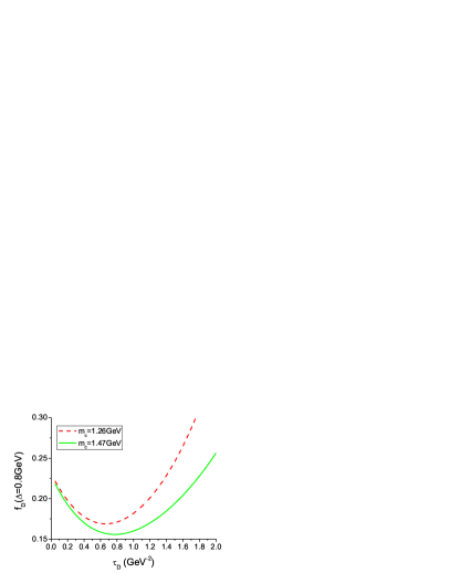
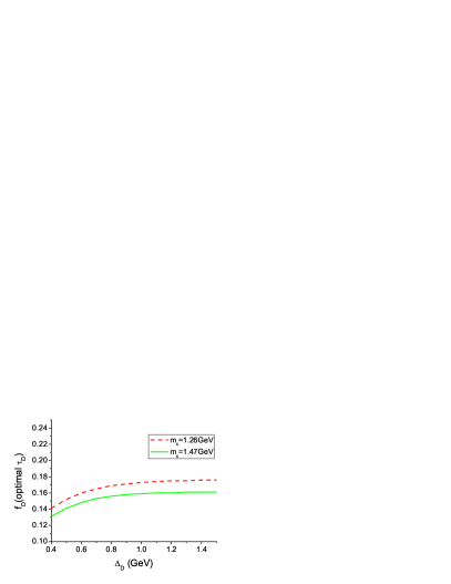
Figure 2: (color online). (a) The two-point SR of $f_{D}$ versus $\tau_{D}$ with $\Delta_{D}=0.8\ \mathrm{GeV}$. The red dashed line is for $m_{c}=1.26\ \mathrm{GeV}$ and the green solid line for $m_{c}=1.47\ \mathrm{GeV}$. (b) $f_{D}$ versus $\Delta_{D}$ with the minimum of $\tau_{D}$ adopted.

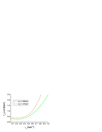
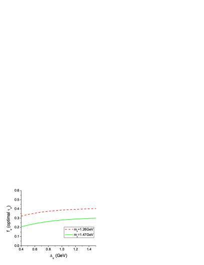
Figure 3: (color online). (a) The two-point SR of $f_{\psi}$ versus $\tau_{\psi}$ with $\Delta_{\psi}=0.8\ \mathrm{GeV}$. The red dashed line is for $m_{c}=1.26\ \mathrm{GeV}$ and the green solid line for $m_{c}=1.47\ \mathrm{GeV}$. (b) $f_{\psi}$ versus $\Delta_{\psi}$ with the minimum of $\tau_{\psi}$ adopted.

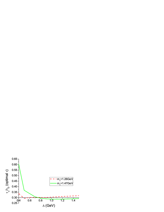
Figure 4: (color online). Behavior of the ratio of SR variables $\tau_{\psi}/\tau_{D}$ versus $\Delta$ for two values of $m_{c}=1.26\ \mathrm{GeV}$ (red dashed line) and $1.47\ \mathrm{GeV}$ (solid green line).

As follows, we adopt $m_{c}=1.26\ \mathrm{GeV}$ and $\Delta_{D}=\Delta_{\psi}\equiv\Delta$ as inputs since it is difficult to find a global maximum with $m_{c}=1.47\ \mathrm{GeV}$ in our three-point SR and the variation of $\tau$ ratio is more stable with $m_{c}=1.26\ \mathrm{GeV}$  ft1 . To obtain more concrete information about the form factor, we consider a large virtuality interval $0\leq-p_{5}^{2}\leq 5\ \mathrm{GeV^{2}}$, which is the same as in Ref. RodriguesdaSilva:2003hh . As an illustration, we show in Fig. 5 the form factor $F_{\psi DD^{*}}(p_{5}^{2})$ at $p_{5}^{2}=-3\ \mathrm{GeV^{2}}$ with both $\Delta\geq 0.4\ \mathrm{GeV}$ and ${\tau_{1}}/{\tau_{2}}=0.3$. For simplicity, $f_{D^{*}}=0.24\ \mathrm{GeV}$ is the same as in Ref. RodriguesdaSilva:2003hh . The ratios of the pole contribution versus the whole dispersion integral are also depicted in Fig. 5 and parameterized as

$$\mathrm{R} \equiv \mathrm{\frac{PI}{WI}},$$ (36)

$$\mathrm{PI} = \int_{4m_{c}^{2}}^{s_{0}}\mathrm{d}s\int_{m_{c}^{2}}^{u_{0}}\mathrm{d}u\,\rho(s,u,Q^{2})$$ (37)

$$\times\theta(u_{\mathrm{max}}-u)\theta(u-u_{\mathrm{min}})e^{-s\tau_{1}-u\tau_{2}},$$

$$\mathrm{WI} = \int_{4m_{c}^{2}}^{\infty}\mathrm{d}s\int_{u_{\mathrm{min}}}^{u_{\mathrm{max}}}\mathrm{d}u\,\rho(s,u,Q^{2})$$ (38)

$$\times\theta(u_{\mathrm{max}}-u)\theta(u-u_{\mathrm{min}})e^{-s\tau_{1}-u\tau_{2}}.$$

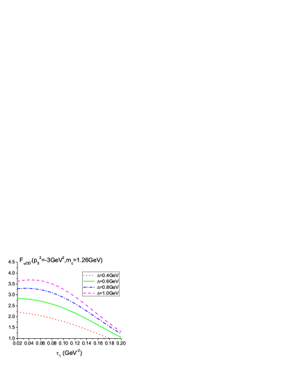
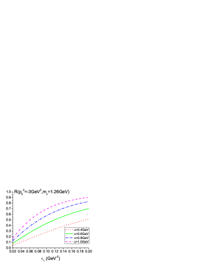
Figure 5: (color online). (a) The $\tau_{1}$ windows of the form factor and (b) the contribution from the corresponding pole at $p_{5}^{2}=-3\ \mathrm{GeV^{2}}$, where $m_{c}=1.26\ \mathrm{GeV}$, $\tau_{1}/\tau_{2}=0.3$, and $\Delta$ as a variable.

With the increase of $\Delta$, the pole contributions will become larger. It is obvious to see that the pole contributions are less than one half at the maximum $\tau_{1}=0.05\ \mathrm{GeV}$ even with $\Delta$ as large as $1\ \mathrm{GeV}$. The situation will be worse with larger $D^{*}$ virtuality. This phenomenon seems to be a common problem for the form factors of charmonium to open charmed mesons. To avoid this difficulty of the SR criterion, we deduce the form factors from Laplace SR varying with different $\Delta$, and also show the predictions from FESR in terms of $\Delta$. In principle, these two SRs should give the same solution, which means that the result at the intersection point is the reliable one from QSSR, see Fig. 6. The form factor from the above method is shown in Fig. 6, and we use three different parameterizations to extend the form factor to broader regions of the $D^{*}$ virtuality:

$$F_{\psi DD^{*}}(p_{5}^{2})=\begin{cases}10.58\exp\left[-\genfrac{}{}{}{0}{(-p_{5}^{2}+21.30)^{2}}{422.62}\right]&\text{Gaussian}\\[10.0pt] \genfrac{}{}{}{0}{332.61}{p_{5}^{4}-8.79p_{5}^{2}+91.98}&\text{Dipole}\\[10.0pt] \genfrac{}{}{}{0}{-25.83}{p_{5}^{2}-7.03}&\textrm{Monopole}\end{cases}$$ (39)

The form factor obtained in Ref. RodriguesdaSilva:2003hh with fixed $f_{\psi}=0.405\ \mathrm{GeV}$, $f_{D}=0.17\ \mathrm{GeV}$, $m_{c}=1.3\ \mathrm{GeV}$, $\Delta_{\psi}=\Delta_{D}=0.5\ \mathrm{GeV}$ and $0.09<\tau_{1}<0.14\ \mathrm{GeV^{-2}}$ are parameterized by the Gaussian formula RodriguesdaSilva:2003hh

$$F_{\psi DD^{*}}(p_{5}^{2})=19.9\exp\left[\frac{-(-p_{5}^{2}+27)^{2}}{345}\right]\,\,.$$ (40)

Below the $D^{*}$ threshold, our improved form factors are slightly larger and decline slower than the one in Ref. RodriguesdaSilva:2003hh . In fact, the form factors used in our following calculation are usually restricted to a small region $-5<p_{5}^{2}<2\ \mathrm{GeV^{2}}$ with on-shell $D$ mesons. Therefore, those different parameterizations would not bring noticeable differences to the calculation results, although in a broader momentum region they turn out to be different from each other especially in the timelike region. Usually, pQCD predicts the power falloff of the form factors, we will use the dipole fit in the following calculations. Notice that there is no real roots, i.e. the unphysical state, in the denominator of our dipole fit (we label it as power fit hereafter to distinguish it from the empirical dipole form factor).

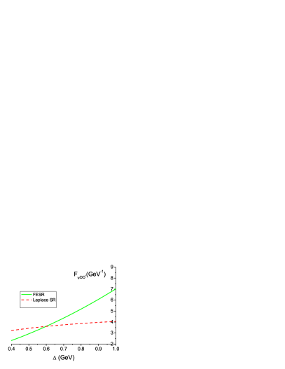
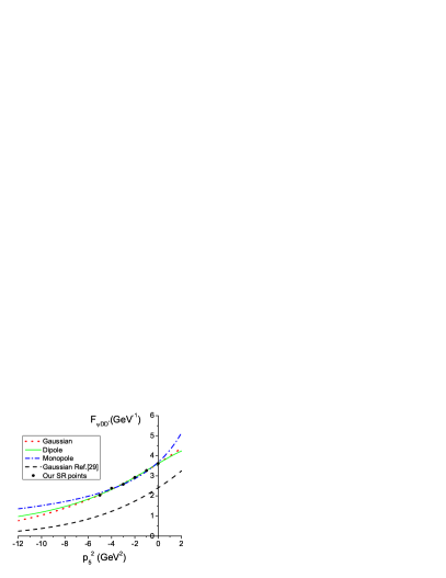
Figure 6: (color online). (a) The intersection point of Laplace SR and FESR at $p_{5}^{2}=0\mathrm{GeV}^{2}$. (b) The $J/\psi DD^{*}$ form factor derived from our method compared with the Gaussian fit  RodriguesdaSilva:2003hh . The blue dash-dotted line is our monopole fit, the green solid line is our dipole fit, the red dotted one is our Gaussian fit, and the black dashed one is the Gaussian fit  RodriguesdaSilva:2003hh . The dots are our SR result.

III.2 The Form factor of $F_{D^{*}D\pi^{0}}(p_{5}^{2})$

As mentioned earlier, the form factor $F_{D^{*}D\pi^{0}}(p_{5}^{2})$ is determined by the $D$ meson semileptonic decays, i.e. $D\to\pi^{0}l\nu$. In the momentum transfer region $p_{5}^{2}<2\ \mathrm{GeV}^{2}$, we expect that the $D^{*}$ pole has the dominant contribution. Thus, the transition matrix element can be expressed as

$$\langle\pi^{0}(p)|\bar{d}\gamma_{\mu}c|D^{+}(p_{4})\rangle$$ (41)

$$\sim \sum_{\epsilon_{5}}\langle\pi^{0}(p)D^{*+}(p_{5})|D^{+}(p_{4})\rangle\langle 0|\bar{d}\gamma_{\mu}c|D^{*+}(p_{5})\rangle\frac{1}{p_{5}^{2}-M_{D^{*+}}^{2}}$$

$$= \frac{F_{D^{*}D\pi^{0}}(p_{5}^{2})M_{D^{*+}}f_{D^{*+}}}{p_{5}^{2}-M_{D^{*+}}^{2}}\left(-p_{\mu}+\frac{p_{5\mu}p\cdot p_{5}}{M_{D^{*+}}^{2}}\right)\ ,$$

where we have used the following definitions consistent with the effective Lagrangian:

$$\langle\pi^{0}(p)D^{*+}(p_{5})|D^{+}(p_{4})\rangle = F_{D^{*}D\pi^{0}}(p_{5}^{2})(p\cdot\epsilon_{5}^{*})\ ,$$

$$\langle 0|\bar{d}\gamma_{\mu}c|D^{*+}(p_{5})\rangle = M_{D^{*+}}f_{D^{*+}}\epsilon_{5\mu}\ .$$ (42)

The transition matrix element of the weak decay can be defined as Khodjamirian:2009ys

$$\langle\pi^{0}(p)|\bar{d}\gamma_{\mu}c|D^{+}(p+p_{5})\rangle = \frac{1}{\sqrt{2}}[(2p+p_{5})_{\mu}f_{+}(p_{5}^{2})+p_{5\mu}f_{-}(p_{5}^{2})]\ ,$$ (43)

where the form factor $f_{+}(p_{5}^{2})$ has been measured with high accuracy, and can be parameterized as a modified pole formula Besson:2009uv

$$f_{+}(p_{5}^{2})=\frac{-f_{+}(0)M_{D^{*}}^{2}}{(p_{5}^{2}-M_{D^{*}}^{2})\left(1-\alpha_{0}\frac{p_{5}^{2}}{M_{D^{*}}^{2}}\right)}\ .$$ (44)

Compared with the $p^{\mu}$ part of the weak decay form factor definition, we obtain the needed form factor:

$$F_{D^{*}D\pi^{0}}(p_{5}^{2})=\frac{\sqrt{2}f_{+}(0)M_{D^{*}}}{\left(1-\alpha_{0}\frac{p_{5}^{2}}{M_{D^{*}}^{2}}\right)f_{D^{*}}}\ ,$$ (45)

where $\alpha_{0}=0.21$ for $D^{0}$, $\alpha_{0}=0.24$ for $D^{+}$ Besson:2009uv , and $f_{+}(0)=0.64$ from the lattice QCD simulations Aubin:2004ej ; Bernard:2009ke for our numerical calculation. Note that $f_{+}(0)$ from QSSR fplusSR are consistent with the lattice result very well. The local coupling $g_{D^{*+}D^{+}\pi^{0}}$ can thus be extracted from the form factor at $p_{5}^{2}=M_{D^{*}}^{2}$ with $f_{D^{*}}=0.24\mathrm{GeV}$, i.e.

$$g_{D^{*}D\pi^{0}}(p_{5}^{2})\equiv F_{D^{*}D\pi^{0}}(p_{5}^{2}=M_{D^{*}}^{2})\simeq 9.97,$$ (46)

which is slightly different from the value extracted from the decay of $D^{*}\rightarrow D+\pi$, i.e. $g_{D^{*}D\pi^{0}}=g_{D^{*}DP}/\sqrt{2}=17.9/\sqrt{2}=12.7$ AA:2001 . One can also extract this coupling from QSSR or QCD light-cone SR. However, both SRs suffer from their inherent uncertainties and the corresponding couplings from most SRs are nearly the same as what we derived from the weak decay form factor. One can refer to Ref. Bracco:2011pg for a review on this issue. Another reason for the discrepancy of the coupling values is that in the momentum transfer region $0<p_{5}^{2}<3\ \mathrm{GeV}^{2}$ which corresponds to the experimental kinematics, the form factor may vary drastically near the pole position of $D^{*}$.

One could of course calculate the dispersive part with empirical form factors, but we must emphasize that in some diagrams containing more $D^{*}$ mesons, e.g. $D^{*}D(D^{*})$ loop in the vector charmonium decay to a $VP$ final state, the empirical dipole form factor used by most of the references is not enough to suppress the ultraviolet divergence in the loops so that we need other more complicated form factors such as the Gaussian form factor. Thus, we leave the direct calculation with empirical form factor aside. We present the empirical dipole form factor (Eq. (10)) with different cutoff in Fig. 7 and compare it with our QCD-motivated form factors. It is obvious that our form factors favor $\alpha>2$, which is consistent with the value used in the study of $X(3872)$ decays Meng:2007cx .

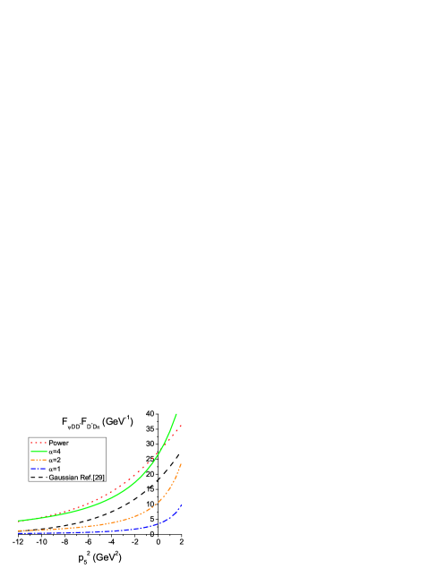
Figure 7: (color online). The QCD induced form factor $F_{\psi DD^{*}}(p_{5}^{2})F_{D^{*}D\pi^{0}}(p_{5}^{2})$ (charged $D$) compared with the empirical dipole form factors. The red dotted line is our power fit, the black dashed line is the form factor obtained in Ref. RodriguesdaSilva:2003hh , the green solid line, the orange dash-dot-dotted line and the blue dash-dotted line correspond to the empirical dipole form factor with $\alpha=4$, $\alpha=2$ and $\alpha=1$, respectively.

IV Numerical results and discussion

The determination of the effective threshold ${th}$ of the dispersive part is not a trivial task. If we know the full information of the spectral density, ${th}$ should be extended to be infinity. Usually, ${th}\equiv(M_{D}+M_{D^{*}})^{2}$ is taken in the literatures as a natural cutoff Meng:2007cx on the assumption that the spectral density can be approximated by the extrapolation of the imaginary part. As an improvement, it is assumed that the corresponding effective threshold of $\psi(3770)\rightarrow J/\psi+\eta$ containing $u,d$ components should be the same as that of $\psi(3770)\rightarrow J/\psi+\pi^{0}$. So, we can determine the effective threshold from the decay width of $\psi(3770)\rightarrow J/\psi+\eta$. The flavor mixing scheme is taken in our calculation, and the mixing angle between $|\bar{n}n\rangle\equiv(|\bar{u}u\rangle+|\bar{d}d\rangle)/\sqrt{2}$ and $|\bar{s}s\rangle$ is $\alpha_{P}\equiv\theta_{P}+\arctan\sqrt{2}\simeq 38^{\circ}$, where $\theta_{P}$ is the mixing angle between the flavor singlet and octet. Note that, as mentioned in the Introduction that the IML contributions are relatively enhanced by $1/v$ in comparison with the tree-level contribution, it leads to the dominance of the IML contributions in $\psi(3770)\to J/\psi+\eta$ which is consistent with the study of Ref. Zhang:2009kr . It can be understood that the isospin violation from the $\eta$-$\pi^{0}$ mixing is different from the IML transitions. In the latter, there is no $\eta$ pole contributions to the strong isospin violations.

In the following calculation of the dispersive part, we will take the SU(3) flavor symmetry for the production of $s\bar{s}$ and $q\bar{q}$ component within the light pseudoscalar mesons. It means the dispersive part of $s\bar{s}$ is approximated by the average of the dispersive integrals of $q\bar{q}$.

The decay constants of $g_{\psi^{\prime\prime}DD}$ in our numerical simulation are listed in Table 1, where $g_{\psi^{\prime\prime}DD}^{low,cen,up}$ correspond to the lower bound, central value, and upper bound allowed by the experimental data Nakamura:2010zzi . From the experimental branching ratio $Br(\psi(3770)\rightarrow J/\psi+\eta)=9\pm 4\times 10^{-4}$Nakamura:2010zzi , we obtain the corresponding $\delta{th}\equiv{th}-(M_{D}+M_{D^{*}})^{2}$ in Tables 2 and  3. One can see that the frequently used natural cutoff $\delta{th}=0$ is not supported by our calculation. Notice that we distinguish the charged and neutral $D(D^{*})$ masses in our numerical calculation. To estimate the uncertainty from $J/\psi DD^{*}$ form factor, we choose our power parametrization and the Gaussian form in Ref. RodriguesdaSilva:2003hh for comparison. The $s_{1}$-dependence of $g_{\psi^{\prime\prime}DD}$ is also taken into account by adding the suppression factor $\exp(-I|\vec{p}_{3}|^{2})$ into the dispersive integral, where $I=0.4\ \mathrm{GeV}^{-2}$ is extracted from the charmonium mass shift Pennington:2007xr . It should be stressed that the dispersive integral with the suppression factor is not considered priority than the original one with a lower effective threshold from the phenomenological viewpoint. Moreover, both imaginary parts numerically decrease faster than $1/s_{1}$, so the unsubtracted dispersion relation used here is self-contained.

In most of the parameter space, the dispersive part of the branching ratio is dominant over the absorptive part for $J/\psi\eta$, while for $J/\psi\pi^{0}$ both absorptive and dispersive parts are important. The difference between different $J/\psi DD^{*}$ form factor is small, despite that the absorptive part of our power fit is systematically larger than the Gaussian fit in Ref. RodriguesdaSilva:2003hh as expected. As shown in Table 2, the branching ratios of $J/\psi\pi^{0}$ obtained from the corresponding effective thresholds are in good agreement with the experimental upper limit $2.8\times 10^{-4}$ Nakamura:2010zzi . As an interesting investigation, we take the threshold asymptotic to infinity with the suppression factor, and the corresponding branching ratios of $J/\psi\pi^{0}$ are still below the upper limit except for $g_{\psi^{\prime\prime}DD}^{low}$. In contrast, the asymptotic limits of $J/\psi\eta$ are far beyond the upper limit of the experiment $13\times 10^{-4}$. Then, even taking the suppression factor into account, the spectral information from other resonances and continuum are still ambiguous, so that the asymptotic limit is questionable and the effective threshold is still necessary.

It is essential to recognize that the isospin symmetry breaking with the vertex couplings is also an important dynamic source apart from effects caused by the mass differences between the charged and neutral $D^{*}$ mesons. In our formulation, the coupling $g_{\psi^{\prime\prime}DD}$ and form factor $F_{D^{*}D\pi^{0}}(p_{5}^{2})$ are extracted from experimental data which suggest different values for the charged and neutral couplings, respectively. Since the form factor $F_{D^{*}D\pi^{0}}(p_{5}^{2})$ can be better fixed by the experimental data, the results listed in Tables 1, 2 and 3 also reflect the effects from the isospin breakings of $g_{\psi^{\prime\prime}DD}$. It is interesting to note that the larger absorptive contributions actually favor smaller difference between the charged and neutral $g_{\psi^{\prime\prime}DD}$ couplings, which is also observed in Refs. Achasov:1994vh ; Achasov:2005qb considering the theoretical Coulomb correction for $g_{\psi^{\prime\prime}DD}$. Taking into account the dispersive part, the central values of $g_{\psi^{\prime\prime}DD}$ give relatively small branching ratios for $\psi^{\prime\prime}\to J/\psi+\pi^{0}$, while deviations from the central values can produce larger branching ratios for $\psi^{\prime\prime}\to J/\psi+\pi^{0}$. Within the present experimental uncertainty bounds Nakamura:2010zzi , the predicted branching ratios for $\psi^{\prime\prime}\to J/\psi+\pi^{0}$ are at the order of $10^{-5}\sim 10^{-4}$. Confirmation of this decay branching ratio would be a strong evidence for the open charm threshold effects in $\psi^{\prime\prime}\to J/\psi+\pi^{0}$. Note that our prediction of the absorptive part is also close to the prediction of Ref. Achasov:2005qb with isospin $I=0$ for $\psi(3770)$, i.e. $Br_{\eta}(\mathrm{Abs})=8\times 10^{-5}$ and $Br_{\pi}(\mathrm{Abs})=2\times 10^{-5}$, which is a consequence of the similar values of the form factors in both approaches.

Table 1: Different $g_{\psi^{\prime\prime}DD}$ from experimental data Nakamura:2010zzi .

	Br ($\psi^{\prime\prime}\rightarrow D^{0}+\bar{D}^{0}$)	Br ($\psi^{\prime\prime}\rightarrow D^{+}+D^{-}$)	$g_{\psi^{\prime\prime}D^{0}\bar{D}^{0}}$	$g_{\psi^{\prime\prime}D^{+}D^{-}}$	Coupling Fraction (N/C)
$g_{\psi^{\prime\prime}DD}^{low}$	0.47	0.45	12.26	14.62	0.84
$g_{\psi^{\prime\prime}DD}^{cen}$	0.52	0.41	12.90	13.95	0.92
$g_{\psi^{\prime\prime}DD}^{up}$	0.57	0.37	13.50	13.25	1.02

Table 2: The branching ratio without suppression factor. “Abs” denotes the absorptive part, and “Tot” is for the sum of the absorptive and dispersive part. The flavor mixing angle is $\alpha_{P}=38^{\circ}$.

	Our power fit			Gaussian fit  RodriguesdaSilva:2003hh
	$g_{\psi^{\prime\prime}DD}^{low}$	$g_{\psi^{\prime\prime}DD}^{cen}$	$g_{\psi^{\prime\prime}DD}^{up}$	$g_{\psi^{\prime\prime}DD}^{low}$	$g_{\psi^{\prime\prime}DD}^{cen}$	$g_{\psi^{\prime\prime}DD}^{up}$
$Br_{\eta}$(Exp)($\times 10^{-4}$)	(5, 13)	(5, 13)	(5, 13)	(5, 13)	(5, 13)	(5, 13)
$Br_{\eta}$(Abs)($\times 10^{-4}$)	2.13	2.16	2.18	1.12	1.14	1.15
$\delta th$($\mathrm{GeV}^{2}$)	(0.17, 1.25)	(0.17, 1.25)	(0.17, 1.25)	(0.9, 2.5)	(0.9, 2.5)	(0.9, 2.5)
$Br_{\pi}$(Abs) ($\times 10^{-4}$)	0.145	0.320	0.558	0.074	0.164	0.287
$Br_{\pi}$(Tot)($\times 10^{-4}$)	(0.46, 1.36)	(0.33, 0.35)	(0.71, 1.13)	(0.49, 1.60)	(0.17, 0.23)	(0.50, 0.81)

Table 3: The branching ratio with suppression factor. “Tot” is for the sum of the absorptive and dispersive part, and “Asym” means we take the asymptotic limit $\delta th\rightarrow\infty$. Flavor mixing angle is $38^{\circ}$.

	Our power fit			Gaussian fit  RodriguesdaSilva:2003hh
	$g_{\psi^{\prime\prime}DD}^{low}$	$g_{\psi^{\prime\prime}DD}^{cen}$	$g_{\psi^{\prime\prime}DD}^{up}$	$g_{\psi^{\prime\prime}DD}^{low}$	$g_{\psi^{\prime\prime}DD}^{cen}$	$g_{\psi^{\prime\prime}DD}^{up}$
$Br_{\eta}$(Exp)($\times 10^{-4}$)	(5, 13)	(5, 13)	(5, 13)	(5, 13)	(5, 13)	(5, 13)
$\delta th$($\mathrm{GeV}^{2}$)	(0.26, 1.60)	(0.26, 1.60)	(0.26, 1.60)	(1.15, 3.50)	(1.15, 3.50)	(1.15, 3.50)
$Br_{\eta}$(Asym) ($\times 10^{-4}$)	84.7	84.7	84.2	35.2	35.2	35.1
$Br_{\pi}$(Abs) ($\times 10^{-4}$)	0.145	0.320	0.558	0.074	0.164	0.287
$Br_{\pi}$(Tot) ($\times 10^{-4}$)	(0.48, 1.49)	(0.33, 0.37)	(0.69, 1.05)	(0.53, 1.73)	(0.18, 0.26)	(0.47, 0.73)
$Br_{\pi}$(Asym) ($\times 10^{-4}$)	13.76	1.47	2.86	5.58	0.62	1.25

V Conclusion

The ELA is very useful to investigate the nature of the near threshold charmonia and charmoniumlike resonances. The largest uncertainty of the ELA comes from the determination of the off-shell effect, i.e. the form factors. In this paper, we investigate the isospin violating decay of $\psi(3770)\to J/\psi+\pi^{0}$. In this process, there is only one $D$-meson loop contributing to the absorptive part, and the form factors encountered in the loop calculation can be relatively well controlled. With the help of QSSR, we extract the $J/\psi DD^{*}$ form factor as an implement from the first principle of QCD. The $DD^{*}\pi^{0}$ form factor can be well determined from the experimental data of $D\rightarrow\pi l\nu$, which has been measured with high accuracy. We also explore the dispersion relation to evaluate the dispersive part of $\psi(3770)$ non-$D\bar{D}$ decays, and find they take an important part in most of the parameter space. It means that the IML effects below the open charmed meson threshold cannot be neglected in general. Different from the traditional natural cutoff of the effective threshold in the dispersive integral, we extract them from the experimental data of $\psi(3770)\rightarrow J/\psi+\eta$. Our prediction of the branching ratio of $\psi(3770)\to J/\psi+\pi^{0}$ is less than $3\times 10^{-5}$ with the couplings $g_{\psi^{\prime\prime}DD}$ extracted from the central values of the data. Within the experimental uncertainty bounds for the extracted $g_{\psi^{\prime\prime}D^{0}\bar{D^{0}}}$ and $g_{\psi^{\prime\prime}D^{+}D^{-}}$, the branching ratio of $\psi(3770)\to J/\psi+\pi^{0}$ can reach the order of $10^{-4}$. Notice that the understanding of the isospin violation of $g_{\psi^{\prime\prime}D\bar{D}}$ is not a trivial task despite the Coulomb correction favors the experimental central value Voloshin:2007dx . It is also suggested that a small admixture of isovector four-quark component of $\psi(3770)$ may also give a measurable decay rate to $J/\psi\pi^{0}$ Voloshin:2005sd . In Ref. Rosner:2004wy the four-quark component is viewed as a reannihilation effect of $D\bar{D}$. To some extent, the nature of $\psi(3770)$ hides in the coupling $g_{\psi^{\prime\prime}DD}$. Meanwhile, the forthcoming BESIII measurement of $\psi(3770)\to J/\psi+\pi^{0}$ will be able to provide useful information about the QCD motivated form factors and clarify the role played by the IML. We plan to discuss the isospin violations with the charged and neutral couplings $g_{\psi^{\prime\prime}D^{+}D^{-}}$ and $g_{\psi^{\prime\prime}D^{0}\bar{D^{0}}}$ elsewhere.

- (1) Y. P. Kuang and T. M. Yan, Phys. Rev. D 41, 155 (1990).
- (2) Y. B. Ding, D. H. Qin and K. T. Chao, Phys. Rev. D 44, 3562 (1991).
- (3) J. L. Rosner, Phys. Rev. D 64, 094002 (2001).
- (4) J. L. Rosner, Annals Phys. 319, 1 (2005).
- (5) E. Eichten, S. Godfrey, H. Mahlke and J. L. Rosner, Rev. Mod. Phys. 80, 1161 (2008).
- (6) M. B. Voloshin, Phys. Rev. D 71, 114003 (2005).
- (7) Q. He et al., Phys. Rev. Lett. 95, 121801 (2005) [Erratum-ibid. 96, 199903 (2006)].
- (8) S. Dobbs et al., Phys. Rev. D 76, 112001 (2007).
- (9) D. Besson et al., Phys. Rev. Lett. 96, 092002 (2006).
- (10) M. Ablikim et al., Phys. Rev. Lett. 97, 121801 (2006).
- (11) Z. G. He, Y. Fan and K. T. Chao, Phys. Rev. Lett. 101, 112001 (2008); M. Ablikim et al., Phys. Lett. B 641, 145 (2006); M. Ablikim et al., Phys. Rev. D 76, 122002 (2007); M. Ablikim et al., Phys. Lett. B 659, 74 (2008).
- (12) Y. -J. Zhang, G. Li, Q. Zhao, Phys. Rev. Lett. 102, 172001 (2009).
- (13) X. Liu, B. Zhang and X. Q. Li, Phys. Lett. B 675, 441 (2009).
- (14) S. L. Olsen, arXiv:0909.2713 [hep-ex].
- (15) K. Nakamura et al. [Particle Data Group], J. Phys. G 37, 075021 (2010).
- (16) D. J. Gross, S. B. Treiman and F. Wilczek, Phys. Rev. D 19, 2188 (1979).
- (17) R. F. Dashen, Phys. Rev. 183, 1245 (1969).
- (18) P. Kroll, Mod. Phys. Lett. A 20, 2667 (2005).
- (19) F. -K. Guo, C. Hanhart and Ulf-G. Meissner, Phys. Rev. Lett. 103, 082003 (2009) [Erratum-ibid. 104, 109901 (2010)].
- (20) F. -K. Guo, C. Hanhart, G. Li, Ulf-G. Meissner and Q. Zhao, Phys. Rev. D 83, 034013 (2011).
- (21) N. N. Achasov and A. A. Kozhevnikov, Phys. Lett. B 260, 425 (1991).
- (22) N. N. Achasov and A. A. Kozhevnikov, Phys. Rev. D 49, 275 (1994).
- (23) N. N. Achasov and A. A. Kozhevnikov, Phys. Atom. Nucl. 69, 988 (2006).
- (24) Q. Wang, G. Li and Q. Zhao, Phys. Rev. D 85, 074015 (2012).
- (25) P. Colangelo, F. De Fazio, T. N. Pham, Phys. Rev. D69, 054023 (2004).
- (26) R. Casalbuoni, A. Deandrea, N. Di Bartolomeo, R. Gatto, F. Feruglio and G. Nardulli, Phys. Rept. 281, 145 (1997).
- (27) R. D. Matheus, F. S. Navarra, M. Nielsen and R. Rodrigues da Silva, Phys. Lett. B 541, 265 (2002).
- (28) M. R. Pennington and D. J. Wilson, Phys. Rev. D 76, 077502 (2007).
- (29) R. Rodrigues da Silva, R. D. Matheus, F. S. Navarra and M. Nielsen, Braz. J. Phys. 34, 236 (2004).
- (30) R. D. Matheus, F. S. Navarra, M. Nielsen and R. Rodrigues da Silva, arXiv:hep-ph/0310280.
- (31) For a review and references to original works, see e.g., S. Narison, QCD as a theory of hadrons, Cambridge Monogr. Part. Phys. Nucl. Phys. Cosmol. 17, 1 (2002); QCD spectral sum rules, Lect. Notes Phys. Vol. 26 (World Scientific, Singapore, 1989), p. 1; Acta Phys. Pol. B 26, 687 (1995); Riv. Nuov. Cim. 10N2, 1 (1987); Phys. Rept. 84, 263 (1982).
- (32) H. G. Dosch, E. Ferreira, M. Nielsen and R. Rosenfeld, Phys. Lett. B 431, 173 (1998).
- (33) This choice could be a posteriori justified as, in different examples, the PT series converge faster when the running quark mass is used instead of the pole mass.
- (34) A. Khodjamirian, C. Klein, T. Mannel and N. Offen, Phys. Rev. D 80, 114005 (2009).
- (35) D. Besson et al. [CLEO Collaboration], Phys. Rev. D 80, 032005 (2009).
- (36) C. Aubin et al. [Fermilab Lattice Collaboration and MILC Collaboration and HPQCD Collab], Phys. Rev. Lett. 94, 011601 (2005).
- (37) C. Bernard et al., Phys. Rev. D 80, 034026 (2009).
- (38) T. M. Aliev, A. A. Ovchinnikov and V. A. Slobodenyuk, Trieste preprint IC/89/382 (1989) (unpublished); P. Ball, Phys. Rev. D 48, 3190 (1993); K. C. Yang and W. Y. P. Hwang, Z. Phys. C 73, 275 (1997).
- (39) S. Ahmed et al. [CLEO Collaboration], Phys. Rev. Lett. 87, 251801 (2001); A. Anastassov et al. [CLEO Collaboration], Phys. Rev. D 65, 032003 (2002).
- (40) M. E. Bracco, M. Chiapparini, F. S. Navarra, M. Nielsen, arXiv:1104.2864 [hep-ph].
- (41) C. Meng and K. T. Chao, Phys. Rev. D 75, 114002 (2007).
- (42) M. B. Voloshin, Prog. Part. Nucl. Phys. 61, 455 (2008).