Stochastic Gravitational Wave Background originating from Halo Mergers

Abstract

The stochastic gravitational wave background (GWB) from halo mergers is investigated by a quasi-analytic method. The method we employ consists of two steps. The first step is to construct a merger tree by using the Extended Press-Schechter formalism or the Sheth & Tormen formalism, with Monte-Carlo realizations. This merger tree provides evolution of halo masses. From $N$-body simulation of two-halo mergers, we can estimate the amount of gravitational wave emission induced by the individual merger process. Therefore the second step is to combine this gravitaional wave emission to the merger tree and obtain the amplitude of GWB. We find $\Omega_{GW}\sim 10^{-19}$ for $f\sim 10^{-17}-10^{-16}$ Hz, where $\Omega_{GW}$ is the energy density of the GWB. It turns out that most of the contribution on the GWB comes from halos with masses below $10^{15}M_{\odot}$ and mergers at low redshift, i.e., $0<z<0.8$.

I Introduction

Stochastic gravitational wave background (GWB) is a valuable source of information for both cosmology and astrophysics.

In the very early universe, inflation Sato (1981); Guth (1981); Albrecht and Steinhardt (1982); Linde (1982) is expected to be the most feasible scenario. It is believed that both scalar and tensor mode perturbations from quantum fluctuations are produced in the epoch of inflation. The former evolve into large scale structure of the universe. And the latter directly travel toward us and are observed as the GWB. Therefore this GWB can be a direct probe of inflation. For that, one needs to solve the transfer of the gravitational wave in the history of the expanding universe from the epoch of inflation to present. For example, Kuroyanagi et al. (2009) studied evolution of the gravitational waves from inflation in detail and showed that the amplitude of the GWB energy spectrum is $\sim 10^{-15}$ for $f>10^{-17}{\rm Hz}$ while the value is very dependent on models of inflation.

The GWB is also produced by second-order scalar perturbations. In the linear perturbations, it is known that structure formation does not generate any gravitaional waves. It turns out that, however, gravitational waves with cosmological scales would be emitted during the process of structure formation if one includes the second-order terms in the perturbation equations as is studied in Mollerach et al. (2004); Ananda et al. (2007); Baumann et al. (2007). The result obtained by them is that the amplitude of the GWB is $10^{-20}-10^{-15}$ for a wide frequency range,

The best method for detecting such GWB with cosmological scales is to measure the B-mode of the Cosmic Microwave Background (CMB). More specifically, the CMB photons are very sensitive to gravitational waves with $f\sim 10^{-17}{\rm Hz}$ Pritchard and Kamionkowski (2005). In actuality, several missions suited for this aim have been planned; for example, ACTPol, SPTpol, POLARBeaR, LiteBIRD (see, http://cmbpol.kek.jp/index-e.html), and Cosmic Inflation Probe (see, http://www.cfa.harvard.edu/cip/). Their primary purpose is to detect primordial gravitational waves generated during inflation.

In this paper, we investigate the GWB originating from dark halo mergers, which are expected to produce gravitational waves with cosmological scales. In a hierarchical model of structure formation, it is expected that low-mass dark halos repeatedly merge with each other, then more massive dark halos are formed (see, e.g., Lacey and Cole (1993, 1994)). A large amounts of gravitational waves from the process would be emitted because the process is a highly nonlinear event. In Inagaki et al. (2010), we studied the gravitational waves emitted from a single galaxy merger with N-body simulations. The peak luminosity and total emitted energy were found to reach about $10^{31}~{}{\rm erg/sec}$ and $10^{47}~{}{\rm erg}$, respectively for a collision of two galaxies with masses $3.8\times 10^{12}M_{\odot}$. We also studied the relative contribution of the disk, bulge and halo, the effect of initial velosity and relative angular momentum. To calculate the GWB, we sum the gravitational wave spectrum from a single merger over the merger history.

This paper is organized as follows: in section 2 our method for calculating the GWB is described; in section 3 we show the results; and in section 4 we provide summary and discussion. In this paper we consider a spatially-flat CDM model with the following cosmological parameters: $\Omega_{m}=0.275,\Omega_{\Lambda}=0.725,h=0.702,\sigma_{8}=0.815$ and $n_{s}=0.963$ for the density parameters of matter and cosmological constant, the hubble constant, the density fluctuation in sphere of $8h^{-1}~{}{\rm Mpc}$ and the spectral index of the primordial scalar fluctuations Komatsu et al. (2011).

II Method

In this section we describe our quasi-analytic method. As the first step, we construct merger history using Monte-Carlo simulation based on the method of Somerville and Kolatt (1999). For the mass function of dark halos, we consider Extended Press-Schechter formalism (EPS) Lacey and Cole (1993, 1994) and Sheth & Tormen formalism (ST) Sheth and Tormen (1999); Jenkins et al. (2001), although the former is mostly used below. In the EPS formalism which provides the conditional mass function, the fraction of the trajectories in haloes with mass $M_{1}$ at $z_{1}$ that are in halos with mass $M_{0}$ at $z_{0}$ $(M_{1}<M_{0},~{}z_{0}<z_{1})$, is given by,

$$f_{\rm PS}(M_{1},z_{1}|M_{0},z_{0})d\sigma_{1}^{2}=$$

$$\frac{1}{\sqrt{2\pi}}\frac{\delta_{c,1}-\delta_{c,0}}{(\sigma_{1}^{2}-\sigma_{0}^{2})^{3/2}}\exp\left[-\frac{(\delta_{c,1}-\delta_{c,0})^{2}}{2(\sigma_{1}^{2}-\sigma_{0}^{2})}\right]d\sigma_{1}^{2},$$ (1)

where $\delta_{c,i}$ and $\sigma_{j}$ are the threshold in the Press-Schechter formalism at time $z_{i}$ and the mass variance for mass $M_{j}$, respectively.

On the other hand, in case of ST, conditional mass function is described by,

$$f_{\rm ST}(M_{1},z_{1}|M_{0},z_{0})d\sigma_{1}^{2}=$$

$$A\sqrt{\frac{a}{2\pi}}\frac{\delta_{c,1}-\delta_{c,0}}{(\sigma_{1}^{2}-\sigma_{0}^{2})^{3/2}}\left[1+\left(\frac{\sigma^{2}_{1}-\sigma^{2}_{0}}{a(\delta_{c,1}-\delta_{c,0})^{2}}\right)^{p}\right]$$

$$\times\exp\left[-\frac{a(\delta_{c,1}-\delta_{c,0})^{2}}{2(\sigma_{1}^{2}-\sigma_{0}^{2})}\right]d\sigma_{1}^{2},$$ (2)

with $A=0.3222$, $a=0.707$ and $p=0.3$.

By using Eqs. (1) and (2), the probability that is a parent halo with mass $M_{1}$ at $z_{1}$ being in a progenitor halo with mass $M_{0}$ at $z_{0}$ is obtained and the merger history can be constructed by performing Monte-Carlo realization according to the conditional mass function. In Fig. 1 mass functions by EPS and ST are shown. One can see that the ST mass function has a larger number of massive halos. Below we use EPS unless otherwise noted.

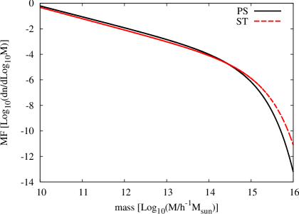
Figure 1: The mass function at present by using EPS(solid) and ST(dashed). The y-axis is the number density in the unit of $1/({\rm h^{-1}Mpc})^{3}$. The x-axis is the halo mass, $M$.

The merger history obtained here provides only evolution of the halo mass and does not give spatial information such as the relative velocity and the angular momentum of halos, which one may consider as important ingredients to estimate the gravitaional wave emission. Fortunately, as we showed in Inagaki et al. (2010), the initial relative velocity does not affect the gravitational wave emission so much. Specifically, the difference in the emitted energies is about $20\%$ between models with zero initial relative velocity and $220~{}{\rm km/s}$ which is the maximum initial relative velocity of two gravitationally-bound halos. On the other hand, the relative angular momentum has a relatively larger effect on the gravitational wave emission. A head-on collision emits three times more energy than a collision where two halos initially have a circular orbit. In the current paper, we assume head-on merger for all the collisions so that our calculation would be over-estimation by a factor less than three.

In constructing the merger history we take the mass resolution $M_{l}=10^{10}h^{-1}M_{\odot}$, that is, we ignore halos with masses less than $M_{l}$ and only consider merger of two halos. The adopted time step of the merger histories is a redshift interval of $\Delta z=0.06(1+z)$, corresponding to the dynamical timescale of halos that collapse at redshift z.

As the second step, we sum up the gravitational waves from dark halo mergers following the merger history obtained above, using the result of Inagaki et al. (2010) which provides the gravitational-wave spectrum from a single merger as a function of the halo masses. This spectral function must cover a wide range of masses and mass ratios and in Inagaki et al. (2010) we found a scaling relation of the spectrum with respect to them. The spectrum of gravitational waves from a merger of equal-mass halos can be written as $E_{GW,0}(f,M_{0})$ where $f$ and $M_{0}$ are the frequency and the fiducial mass. The energy spectrum for a given mass $M$ can be decribed by,

$$E_{GW}(f,M)=\left(\frac{M}{M_{0}}\right)^{1+\frac{7}{\alpha}}E_{GW,0}\left(\left(\frac{M}{M_{0}}\right)^{1-\frac{3}{\alpha}}f,M_{0}\right),$$ (3)

where $\alpha=3.4$. The energy spectrum in the case of unequal masses, $M_{1}$ and $M_{2}$, can be obtained by replacing $M$ in the Eq. (3) with $\sqrt{M_{1}M_{2}}$. Here we set $M_{0}=3.8\times 10^{12}h^{-1}M_{\odot}$ and then the total energy is $E_{GW,0}=5\times 10^{46}~{}h^{-1}{\rm erg}$.

Here we demonstrate how valid the scaling relation Eq. (3) is. Fig. 2 shows the energy spectra of the emitted gravitational waves in the logarithmic spacing, i.e, $fE(f)$ for three equal-mass mergers with $M=3.8\times 10^{12}$, $3.8\times 10^{11}$ and $3.8\times 10^{10}~{}h^{-1}M_{\odot}$. The top panel is the original spectra and the bottom panel is the spectra scaled by Eq. (3) to fit with the case with $M=3.8\times 10^{12}h^{-1}M_{\odot}$. In these cases, the error of the scaling relation is less than $40\%$. It should be noticed that the energy spectrum has a peak between $10^{-17}$ to $10^{-15}{\rm Hz}$ which corresponds to the dynamical time scale of halo merger, $\sim 1{\rm Gyr}$.

Fig. 3 is a demonstration for mergers of unequal-mass halos. Here we fix the higher mass to $3.8\times 10^{12}h^{-1}M_{\odot}$ and vary the mass ratio as $1:1$, $1:1/10$ and $1:1/100$. The top panel in Fig. 3 shows the original spectra and the bottom panel shows the spectra scaled by Eq. (3). Although the error of the scaling relation is relatively large at high frequencies ($>10^{-16}~{}{\rm Hz}$), it is still reasonable at low frequencies where most of the energy is emitted. Thus, we use Eq. (3) as a reasonable scaling relation for both equal- and unequal-mass mergers.

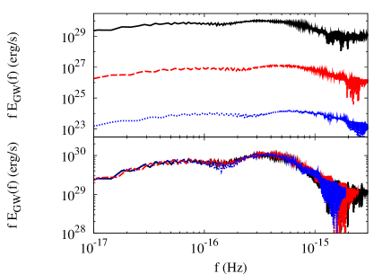
Figure 2: The energy spectra of the gravitational waves in the logarithmic spacing for mergers of equal-mass halos, $M/h^{-1}M_{\odot}=3.8\times 10^{12}$ (solid line), $3.8\times 10^{11}$ (dashed line) and $3.8\times 10^{10}$ (dotted). Y-axis is the energy spectra of the gravitational waves from a merger in the unit of $h^{-1}{\rm erg/s}$. Top: the original spectra. Bottom: the spectra scaled by Eq. (3).

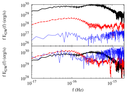
Figure 3: The energy spectra of the gravitational waves in the logarithmic spacing for mergers of unequal-mass halos. The solid line shows the case of a merger of equal-mass halos $M/h^{-1}M_{\odot}=3.8\times 10^{12}$ shown for comparison. The dashed and doted lines show the cases of unequal masses (dashed line:$M/h^{-1}M_{\odot}=3.8\times 10^{11}$ and $3.8\times 10^{12}$, dotted line: $M/h^{-1}M_{\odot}=3.8\times 10^{10}$ and $3.8\times 10^{12}$). Y-axis is the energy spectra of the gravitational waves from a merger in the unit of $h^{-1}{\rm erg/s}$. Top: the original spectra. Bottom: the spectra scaled by Eq. (3).

The energy density of the GWB at redshift $z_{i}$ can be calculated as,

$$\rho_{GW}(f,z_{i})=\frac{1}{V_{\rm com}}\sum_{N_{i}}E^{(N_{i})}_{GW}(f),$$ (4)

where $V_{\rm com}$ is a comoving volume and $N_{i}$ represents the $N_{i}$-th merger in the $i$-th redshift bin. It should be noted that, due to the expansion of the universe, the frequency and the energy density of the gravitational waves are redshifted as $f\propto 1/(1+z)$ and $\rho_{GW}\propto 1/(1+z)^{4}$, respectively. Therefore, the energy density $\rho_{GW}$ at $z=0$ can be written as,

$$\rho_{GW}(\tilde{f},z=0)=\frac{1}{V_{\rm phys}}\sum_{i}\sum_{N_{i}}\frac{1}{1+z_{i}}E^{(N_{i})}_{GW}(\tilde{f}),$$ (5)

where $\tilde{f}$ and $V_{\rm phys}$ show the redshifted frequency and a physical volume, respectively. Finally, the density parameter of the GWB, $\Omega_{GW}$, is defined as,

$$\Omega_{GW}(\tilde{f})\equiv\frac{1}{\rho_{c,0}c^{2}}\left|\frac{d\rho_{GW}(\tilde{f},z=0)}{d\ln\tilde{f}}\right|,$$ (6)

where $\rho_{c,0}$ and $c$ show the critical density of the universe at present and the speed of light, respectively.

III Results

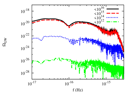
Figure 4: The GWB spectra for each mass range. The solid, dashed and dotted lines are mass range of $M/h^{-1}M_{\odot}\leq 10^{16}$, $10^{15}$, $10^{14}$ and $10^{12}$, respectively.

We obtain the spectrum of the GWB by using the method described in the previous section. First we show the dependence of the result with respect to the upper-cutoff mass $M_{\rm cut}$ of halos. Fig. 4 represents the GWB spectra for several mass cutoffs, $10^{16}h^{-1}M_{\odot}$, $10^{15}h^{-1}M_{\odot}$, $10^{14}h^{-1}M_{\odot}$ and $10^{12}h^{-1}M_{\odot}$. The emitted energy reaches $\Omega_{GW}\sim 5\times 10^{-20}$ for $M_{\rm cut}\leq 10^{16}h^{-1}M_{\odot}$ and the spectral shape is very similar to that of a single merger shown in Fig. 2. The difference in the spectra is very small for the cases with $M_{\rm cut}=10^{15}h^{-1}M_{\odot}$ and $10^{16}h^{-1}M_{\odot}$. This can be easily understood by the shape of the mass function in Fig. 1, where the number of halos steeply decreases above $10^{15}h^{-1}M_{\odot}$. On the other hand, the difference is about two orders of magnitude between the cases with $M_{\rm cut}=10^{14}M_{\odot}$ and $10^{15}h^{-1}M_{\odot}$, which implies that most of GWB energy is contributed from mergers of massive halos. Because the GWB spectrum is saturated at $M_{\rm cut}=10^{15}h^{-1}M_{\odot}$, we take $10^{15}h^{-1}M_{\odot}$ as a cutoff mass hereafter.

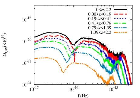
Figure 5: Contributions of several redshift ranges to the GWB spectrum.

Figure 6: The total number of merger at each redshift. The assumed volume is $(6~{}h^{-1}{\rm Gyr})^{3}$ correspoding to hubble scale.

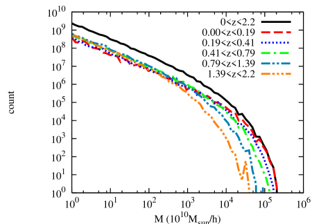
Figure 7: The number of mergers at each redshift with respect to mass that is higher mass of two merger haloes. The assumed volume is $(6~{}h^{-1}{\rm Gyr})^{3}$ correspoding to hubble scale.

Next we investigate the relative contributions of redshift ranges to the GWB spectrum. In Fig. 5, the contributions from several redshift bins are shown. The widths of the bins are determined so that each bin corresponds to the same cosmic time interval of $2~{}{\rm Gyr/h}$. Each spectrum in Fig. 5 represents the GWB emitted by mergers in each redshift range. Due to the redshift of gravitational wave, contributions from larger $z$ bins have peaks at lower frequencies. We find $46\%$ of the total energy of the gravitational waves comes from the redshift interval $0\leq z\leq 0.19$, while the gravitational waves from the $0.19\leq z\leq 0.41$ and $0.41\leq z\leq 0.79$ contribute to the GWB spectrum by about $26\%$ and $15\%$, respectively. Thus, about $90\%$ of the GWB comes from the redshift interval $0\leq z\leq 0.79$.

To understand this behavior, we show the merger rate below. Fig. 6 represents the total number of halo mergers for each redshift bin of Fig. 5. The total number has a peak at $0.79<z<1.39$ and decreases toward lower $z$. However, as can be seen in Fig. 7 which represents the merger rate as a function of mass, mergers of massive halos takes place more frequent for lower $z$. This would be natural in the hierarchical scenario of structure formation. Because the energy of emitted graviational waves increases substantially with the halo masses (see Eq. (3)), the dominant contribution to the resultant spectrum of GWB comes from the lowest-redshift bin although the total number of mergers is relatively small. Here we remark that we have checked that the contribution from $z>2.2$ is negligible as expected.

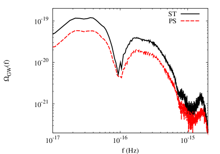
Figure 8: The spectrum by using ST(solid) and EPS(dashed).

Finally, we compare the spectra of the GWB calculated using EPS and ST mass functions in Fig. 4. Here we took the cutoff mass $M_{\rm cut}=10^{16}h^{-1}M_{\odot}$. The total energy of the GWB for ST case is larger than that for EPS case by a factor of two and reaches $\Omega_{GW}\sim 10^{-19}$. This is because massive halos are more abundant for ST than EPS.

IV Summary and Discussion

In this paper, we calculated the spectrum of gravitational wave background originating from dark halo mergers by a quasi-analytic method. First, we constructed merger histories by Monte-Carlo realizations for a mass function (Extended Press-Schechter formalism or the Sheth & Tormen formalism). Then we summed up the energy spectra from halo mergers following the merger history, using the result of Inagaki et al. (2010) which provides the gravitational-wave spectrum from a single merger as a function of the halo masses. We found that the energy density reaches $\Omega_{GW}\sim 5\times 10^{-20}$ and that the dominant contribution comes from mergers of massive halos $10^{14}-10^{15}h^{-1}M_{\odot}$ at relatively low redshifts $z<0.19$. We gave an interpretation of the relative importance of ranges of halo masses and redshifts showing the merger rates as a function of mass and redshift. We also compared the GWB spectra obtained by EPS to ST mass functions and found that the latter case has larger energy by a factor of two.

Finally, we discuss the observability of the GWB from halo mergers. Stochastic gravitational wave background converts the E-mode polarization of CMB into the B-mode through gravitational lensing between the observer and the last scattering. Thus observation of B-mode would be useful to probe GWs after last scattering. The energy of the GWB is at most $\Omega_{GW}\sim 10^{-19}$ according to our calculations. This corresponds to inflationary gravitational waves with the tensor-to-scalar ratio $r\sim 10^{-4}$ Kuroyanagi et al. (2009). It may be possible to detect them through B-mode polarization of CMB if the tensor-to-scalar ratio is lower than above the value. In this case, our result would be useful to probe the process of structure formation.