Fast projections onto mixed-norm balls with applications

Abstract

Joint sparsity offers powerful structural cues for feature selection, especially for variables that are expected to demonstrate a “grouped” behavior. Such behavior is commonly modeled via group-lasso, multitask lasso, and related methods where feature selection is effected via mixed-norms. Several mixed-norm based sparse models have received substantial attention, and for some cases efficient algorithms are also available. Surprisingly, several constrained sparse models seem to be lacking scalable algorithms. We address this deficiency by presenting batch and online (stochastic-gradient) optimization methods, both of which rely on efficient projections onto mixed-norm balls. We illustrate our methods by applying them to the multitask lasso. We conclude by mentioning some open problems.

Keywords: Mixed-norm, Group sparsity, Fast projection, multitask learning, matrix norms, stochastic gradient

1 Introduction

Sparsity encodes key structural information about data and permits estimating unknown, high-dimensional vectors robustly. No wonder, sparsity has been intensively studied in signal processing, machine learning, and statistics, and widely applied to many tasks therein. But the associated literature has grown too large to be summarized here; so we refer the reader to [36, 2, 35, 28] as starting points.

Sparsity constrained problems are often cast as instances of the following high-level optimization problem

$$\min\nolimits_{x\in\mathbb{R}^{d}}\quad L(x)+\lambda f(x),$$ (1.1)

where $L$ is a differentiable loss-function, $f$ is a convex (nonsmooth) regularizer, and $\lambda>0$ is a scalar. Alternatively, one may prefer the constrained formulation

$$\min\nolimits_{x\in\mathbb{R}^{d}}\quad L(x)\quad\text{s.t.}\quad f(x)\leq\gamma.$$ (1.2)

Both formulations (1.1) and (1.2) continue to be actively researched, the former perhaps more than the latter. We focus on the latter, primarily because it often admits simple but effective first-order optimization algorithms. Additional benefits that make this constrained formulation attractive include:

• Even when the loss $L$ is nonconvex, gradient-projection remains applicable;

• If the loss is separable, it is easy to derive highly scalable incremental or stochastic-gradient based optimization algorithms;

• If only inexact projections onto $f(x)\leq\gamma$ are possible (a realistic case), convergence analysis of gradient-projection-type methods remains relatively simple.

In this paper, we study a particular subclass of (1.2) that has recently become important, namely, groupwise sparse regression. Two leading examples are multitask learning [16, 15, 24, 30] and group-lasso [45, 44, 3]. A key component of these regression problems is the regularizer $f(x)$, which is designed to enforce ‘groupwise variable selection’—for example, with $f(x)$ chosen to be a mixed-norm.

Definition 1 (Mixed-norm).

Let $x\in\mathbb{R}^{d}$ be partitioned into subvectors $x^{i}\in\mathbb{R}^{d_{i}}$, for $i\in[m]$. The $\ell_{p,q}$-mixed-norm for $p$, $q\geq 1$, is then defined as

$$f(x)=\|{x}\|_{p,q}:=\bigl{(}\sum\nolimits_{i=1}^{m}\|{x^{i}}\|_{q}^{p}\bigr{)}^{1/p}.$$ (1.3)

The most practical instances of (1.3) are $\ell_{1,q}$-norms, especially for $q\in\left\{{1,2,\infty}\right\}$. The choice $q=1$ yields the ordinary $\ell_{1}$-norm penalty; $q=2$ is used in group-lasso [45], while $q=\infty$ arises in compressed sensing [43] and multitask lasso [24]. Less common, though potentially useful versions allow interpolating between these extremes by letting $q\in(1,\infty)$; see also [34, 46, 22].

Definition 1 can be substantially generalized: we may allow the subvectors $x^{i}$ to overlap; or to even be normed differently [47]. But unless the overlapping has special structure [19, 28, 27], it leads to somewhat impractical mixed-norms, as the corresponding optimization problem (1.2) becomes much harder. Since our chief aim is to develop fast, scalable algorithms for (1.2), we limit our discussion to $\ell_{1,q}$-norms—this choice is widely applicable, hence important [44, 24, 17, 20, 5, 40, 14, 30, 15].

Before moving onto the technical part, we briefly list the paper’s main contents:

• Batch and online (stochastic-gradient based) algorithms for solving (1.2);

• Theory of and algorithms for fast projection onto $\ell_{1,q}$-norm balls;

• Application to $\ell_{1,q}$-norm based multitask lasso; both batch and online versions;

• Application to computing projections for matrix mixed-norms;

• A set of open problems.

2 Basic theory

We begin by developing some basic theory. Our aim is to efficiently implement a generic ‘first-order’ algorithm: Generate a sequence $\left\{{x_{t}}\right\}$ by iterating

$$x_{t+1}=\text{proj}_{f}(x_{t}-\eta_{t}\nabla_{t}),\quad t=0,1,\ldots,$$ (2.1)

where $\eta>0$ is a stepsize, $\nabla_{t}$ is an estimate of the gradient, and $\text{proj}_{f}$ is the projection operator that enforces the constraint $f(x)\leq\gamma$. Below we expand on the most challenging component of iteration (2.1) when applied to mixed-norm regression, namely efficient computation of the projection operator $\text{proj}_{f}$.

2.1 Efficient projection via proximity

Formally, the (orthogonal) projection operator $\text{proj}_{f}:\mathbb{R}^{d}\to\mathbb{R}^{d}$ is defined as

$$\text{proj}_{f}(y):=\operatorname*{argmin}\nolimits_{x}\quad\tfrac{1}{2}\|{x-y}\|_{2}^{2}\quad\text{s.t.}\quad f(x)\leq\gamma.$$ (2.2)

Closely tied to projection is the proximity operator $\operatorname{prox}_{h}:\mathbb{R}^{d}\times\mathbb{R}_{+}\to\mathbb{R}^{d}$

$$\hskip-34.14322pt\operatorname{prox}_{h}(y,\theta):=\operatorname*{argmin}\nolimits_{x}\quad\tfrac{1}{2}\|{x-y}\|_{2}^{2}+\theta h(x),$$ (2.3)

where $h$ is a convex function on $\mathbb{R}^{d}$. Operator (2.3) generalizes projections: if in (2.3) the function $h$ is chosen to be the indicator function for the set $\left\{{x:f(x)\leq\gamma}\right\}$, then the operator $\operatorname{prox}_{h}$ reduces to the projection operator $\text{proj}_{f}$.

Alternatively, for convex $f$ and $h$, operators $\text{proj}_{f}$ and $\operatorname{prox}_{h}$ are also intimately connected by duality. Indeed, this connection proves key to computing a projection efficiently whenever its corresponding proximity operator is ‘easier’. The idea is simple (see e.g., [31]), but exploiting it effectively requires some care; let us see how.

Let $\mathcal{L}(x,\theta)$ be the Lagrangian for (2.2); and let the optimal dual solution be denoted by $\theta^{*}$. Assuming strong-duality, the optimal primal solution is given by

$$x(\theta^{*}):=\operatorname*{argmin}\nolimits_{x}\ \mathcal{L}(x,\theta^{*}):=\operatorname*{argmin}\nolimits_{x}\ \tfrac{1}{2}\|{x-y}\|_{2}^{2}+\theta^{*}(f(x)-\gamma).$$ (2.4)

But to compute (2.4), we require the optimal $\theta^{*}$—the key insight on obtaining $\theta^{*}$ is that it can be computed by solving a single nonlinear equation. Here is how.

First, observe that if $f(y)\leq\gamma$, then $x(\theta^{*})=y$, and there is nothing to compute. Thus, assume that $f(y)>\gamma$; then, the optimal point $x(\theta^{*})$ satisfies

$$f(x(\theta^{*}))=\gamma.$$ (2.5)

Next, observe from (2.4) that for a fixed $\theta$, the point $x(\theta)$ equals the operator $\operatorname{prox}_{f}(y,\theta)$. Consider, therefore, the nonlinear function (residual)

$$g(\theta):=f(x(\theta))-\gamma\ =\ f(\operatorname{prox}_{f}(y,\theta))-\gamma,$$ (2.6)

which measures how accurately equation (2.5) is satisfied. The optimal $\theta^{*}$ can be then obtained by solving $g(\theta)=0$, for which the following lemma proves very useful.

Lemma 2.

Let $f(x)$ be a gauge, and let $g(\theta)$ be as defined in (2.6). Then, there exists an interval $[0,\theta_{\max}]$, on which $g(\theta)$ is monotonically decreasing, and differs in sign at the endpoints.

Proof.

By assumption on $f(y)$, it holds that $g(0)=f(y)-\gamma>0$. We claim that for $\theta\geq{f}^{\circ}(y)$, where ${f}^{\circ}$ denotes the polar of $f$, the optimal point $x(\theta)=0$. To see why, suppose that $\theta\geq{f}^{\circ}(y)$, but $x(\theta)\neq 0$. Then, $\tfrac{1}{2}\|{x(\theta)-y}\|_{2}^{2}+\theta f(x(\theta))<\tfrac{1}{2}\|{y}\|_{2}^{2}$. But since $\|{\cdot}\|_{2}^{2}$ is strictly convex, the inequality $\|{y}\|_{2}^{2}-\|{x-y}\|_{2}^{2}<2\langle{y},\,{x}\rangle$ also holds for any $x$. Thus, it follows that $\theta<\langle{y},\,{x(\theta)}\rangle/f(x(\theta))$, whereby, for $\theta\geq\sup_{x\neq 0}{\langle{y},\,{x}\rangle}/{f(x)}={f}^{\circ}(y)$, the optimal $x(\theta)$ must equal $0$. Hence, we may select $\theta_{\max}={f}^{\circ}(y)$. Monotonicity of $g$ follows easily, as it is the derivative of the concave (dual) function $\inf_{x}\mathcal{L}(x,\theta)$. Finally, $g(\theta_{\max})=-\gamma<0$, so it differs in sign.∎∎

Since $g(\theta)$ is continuous, changes sign, and is monotonic in the interval $[0,\theta_{\max}]$, it has a unique root therein. This root can be computed to $\epsilon$-accuracy using bisection in $O(\log(\theta_{\max}/\epsilon))$ iterations. We recommend not to use mere bisection, but rather to invoke a more powerful root-finder that combines bisection, inverse quadratic interpolation, and the secant method (e.g., Matlab’s fzero function). Pseudocode encapsulating these ideas is given in Algorithm 1.

Input: Subroutine to compute $\operatorname{prox}_{f}(y,\theta)$; vector $y$; scalar $\gamma>0$

Output: $x^{*}:=\text{proj}_{f}(y,\gamma)$

if $f(y)\leq\gamma$ then

      return $x^{*}=y$

else

       Define $g(\theta):=\operatorname{prox}_{f}(y,\theta)-\gamma$;

       Compute interval $[\theta_{\min},\theta_{\max}]=[0,{f}^{\circ}(y)]$;

       Compute root $\theta^{*}=\textsc{FindRoot}(g(\theta),\theta_{\min},\theta_{\max})$;

      

return $x^{*}=\operatorname{prox}_{f}(y,\theta^{*})$

Algorithm 1 Root-finding for projection via proximity

2.1.1 Projection onto $\ell_{1,q}$-norm balls

After the generic approach above, let us specialize to projections for the case of central interest to us, namely, $\text{proj}_{f}$ with $f(x)=\ell_{1,q}(x)$. Algorithm 1 requires computing the upper bound $\theta_{\max}={f}^{\circ}(y)$. To that end Lemma 3, which actually proves much more, proves useful.

Lemma 3 (Dual-norm).

Let $p,q\geq 1$; and let $p^{*},q^{*}\geq 1$ be “conjugate” scalars, i.e., $1/p+1/p^{*}=1$ and $1/q+1/q^{*}=1$. The polar (dual-norm) of $\|{\cdot}\|_{p,q}$ is $\|{\cdot}\|_{p^{*},q^{*}}$.

Proof.

By definition, the norm dual to an arbitrary norm $\|{\cdot}\|{}$ is given by

$$\|{u}\|_{*}:=\sup\left\{{\langle{x},\,{u}\rangle\ |\ \ \|{x}\|{}\leq 1}\right\}.$$ (2.7)

To prove the lemma, we prove two items: (i) for any two (conformally partitioned) vectors $x$ and $u$, we have $|\langle{x},\,{u}\rangle|\leq\|{x}\|_{p,q}\|{u}\|_{p^{*},q^{*}}$; and (ii) for each $u$, there exists an $x$ for which $\langle{x},\,{u}\rangle=\|{y}\|_{p^{*},q^{*}}$.

Let $x$ be a vector partitioned conformally to $u$, and consider the inequality

$$\langle{x},\,{u}\rangle=\sum\nolimits_{i=1}^{g}\langle{x^{i}},\,{u^{i}}\rangle\leq\sum\nolimits_{i=1}^{g}\|{x^{i}}\|_{q}\|{u^{g}}\|_{q^{*}},$$ (2.8)

which follows from Hölder’s inequality. Define $\psi=[\|{x^{i}}\|_{q}]$ and $\xi=[\|{u^{i}}\|_{q^{*}}]$, and invoke Hölder’s inequality again to obtain $\langle{\psi},\,{\xi}\rangle\leq\|{\psi}\|_{p}\|{\xi}\|_{p^{*}}=\|{x}\|_{p,q}\|{u}\|_{p^{*},q^{*}}$. Thus, from definition (2.7) we conclude that $\|{u}\|_{*}\leq\|{u}\|_{p^{*},q^{*}}$. To prove that the dual norm actually equals $\|{u}\|_{p^{*},q^{*}}$, we show that for each $u$, we can find an $x$ that satisfies $\|{x}\|_{p,q}=1$, for which the inner-product $\langle{x},\,{u}\rangle=\|{u}\|_{p^{*},q^{*}}$.

Define therefore $\beta=\sum_{i}\|{u^{i}}\|_{q^{*}}^{p^{*}}$—some juggling with indices suggests that we should set

$$x_{j}^{i}=\frac{1}{\beta^{1/p}}\frac{\|{u^{i}}\|_{q^{*}}^{p^{*}}}{\|{u^{i}}\|_{q^{*}}^{q^{*}}}\operatorname{sgn}(u^{i}_{j})|u^{i}_{j}|^{q^{*}-1},$$ (2.9)

where $x^{i}_{j}$ denotes the $j$-the element of the subvector $x^{i}$ (similarly $u^{i}_{j}$). To see that (2.9) works, first consider the inner-product

$$\langle{x},\,{u}\rangle=\sum\nolimits_{i}\langle{x^{i}},\,{u^{i}}\rangle =\sum\nolimits_{i}\sum\nolimits_{j}x^{i}_{j}u^{i}_{j}$$

$$=\frac{1}{\beta^{1/p}}\sum\nolimits_{i}\|{u^{i}}\|_{q^{*}}^{p^{*}-q^{*}}\sum\nolimits_{j}|u^{i}_{j}|^{q*}\qquad(\text{since }\operatorname{sgn}(u^{i}_{j})u^{i}_{j}=|u^{i}_{j}|)$$

$$=\frac{1}{\beta^{1/p}}\sum\nolimits_{i}\|{u^{i}}\|_{q^{*}}^{p^{*}}=\frac{\beta}{\beta^{1/p}}=\beta^{1-1/p}=\beta^{1/p^{*}}$$

$$=\left(\sum\nolimits_{i}\|{u^{i}}\|_{q^{*}}^{p^{*}}\right)^{1/p^{*}}=\|{u}\|_{p^{*},q^{*}}.$$

Next, we check that $\|{x}\|_{p,q}=\left(\sum_{i}\|{x^{i}}\|_{q}^{p}\right)^{1/p}=1$. Consider thus, the term $\|{x^{i}}\|_{q}^{p}=\bigl{(}\sum_{j}|x^{i}_{j}|^{q}\bigr{)}^{p/q}$. Using (2.9) we have

$$\sum\nolimits_{j}|x^{i}_{j}|^{q} =\frac{1}{\beta^{q/p}}\|{u^{i}}\|_{q^{*}}^{(p^{*}-q^{*})q}\sum\nolimits_{j}|u^{i}_{j}|^{q(q^{*}-1)}$$

$$=\frac{1}{\beta^{q/p}}\|{u^{i}}\|_{q^{*}}^{(p^{*}-q^{*})q}\sum\nolimits_{j}|u^{i}_{j}|^{q^{*}}\qquad (\text{since }q^{*}q^{-1}+1=q^{*})$$

$$=\frac{1}{\beta^{q/p}}\|{u^{i}}\|_{q^{*}}^{(p^{*}-q^{*})q+q^{*}}=\frac{1}{\beta^{q/p}}\|{u^{i}}\|_{q^{*}}^{p^{*}q-q^{*}(q-1)}$$

$$=\frac{1}{\beta^{q/p}}\|{u^{i}}\|_{q^{*}}^{(p^{*}-1)q} \qquad(\text{since }q(q^{*})^{-1}+1=q).$$

Thus, it follows that

$$\|{x^{i}}\|_{q}^{p}=\Bigl{(}\sum\nolimits_{j}|x^{i}_{j}|^{q}\Bigr{)}^{p/q}=\frac{1}{\beta}\|{u^{i}}\|{q^{*}}^{p(p^{*}-1)}=\frac{1}{\beta}\|{u^{i}}\|{q^{*}}^{p^{*}},$$ (2.10)

where the last equality holds because $1/p+1/p^{*}=1$. Finally, from (2.10) it follows that

$$\|{x}\|_{p,q}=\bigl{(}\sum\nolimits_{i}\|{x^{i}}\|_{q}^{p}\bigr{)}^{1/p}=\bigl{(}\tfrac{1}{\beta}\sum\nolimits_{i}\|{u^{i}}\|_{q^{*}}^{p^{*}}\bigr{)}^{1/p}=1,$$ (2.11)

since by definition $\beta=\sum_{i}\|{u^{i}}\|_{q^{*}}^{p^{*}}$. This concludes the proof. ∎

The next key component for Algorithm 1 is the proximity operator $\operatorname{prox}_{f}$. For $f(x)=\|{x}\|_{1,q}$, this operator requires solving

$$\min_{x^{1},\ldots,x^{m}}\ \sum\nolimits_{i=1}^{m}\tfrac{1}{2}\|{x^{i}-y^{i}}\|_{2}^{2}+\theta\sum\nolimits_{i=1}^{m}\|{x^{i}}\|_{q}.$$ (2.12)

Fortunately, Problem (2.12) separates into a sum of $m$ independent, $\ell_{q}$-norm proximity operators. It suffices, therefore, to only consider a subproblem of the form

$$\min\nolimits_{u}\quad\tfrac{1}{2}\|{u-v}\|_{2}^{2}+\theta\|{u}\|_{q}.$$ (2.13)

For $q=1$, the solution to (2.13) is given by the soft-thresholding operation [13]:

$$u(\theta)=\operatorname{sgn}(v)\odot\max(|v|-\theta,0),$$ (2.14)

where operator $\odot$ performs elementwise multiplication. For $q=2$, we get

$$u(\theta)=\max(1-\theta\|{v}\|_{2}^{-1},0)v,$$ (2.15)

while the case $q=\infty$ is slightly more involved. It can be solved via the Moreau decomposition [11], which, for a norm $f=\|{\cdot}\|$ implies that

$$\operatorname{prox}_{f}(v,\theta)=v-\text{proj}_{{f}^{\circ}}(v,\theta).$$ (2.16)

For $f=\|{\cdot}\|_{\infty}$, the dual-norm (polar) is ${f}^{\circ}=\|{\cdot}\|_{1}$; but projection onto $\ell_{1}$-balls has been extremely well-studied—see e.g., [29, 21, 25].

For $q>1$ (different from $2$ and $\infty$), problem (2.13) is much harder. Fortunately, this problem was recently solved in [26], using nested root-finding subroutines. But unlike the cases $q\in\left\{{1,2,\infty}\right\}$, the proximity operator for general $q$ can be computed only approximately (i.e., in (2.6), each iteration generates only approximate $x(\theta)$).

2.1.2 Mixed norms for matrices: a brief digression

We now make a brief digression, which is afforded to us by the above results. Our digression concerns mixed-norms for matrices, as well as their associated projection, proximity operators, which ultimately depend on the results of the previous section.

Our discussion is motivated by applications in [42], where the authors used mixed-norms on matrices to simultaneously. We define mixed-norms on matrices by building upon the classic Schatten-$q$ matrix norms [7], defined as:

$$\|{X}\|_{q}:=\bigl{(}\sum\nolimits_{i}\sigma_{i}^{q}(X)\bigr{)}^{1/q},\quad\text{for}\ q\geq 1,$$ (2.17)

where $X$ is an arbitrary complex matrix, and $\sigma_{i}(X)$ is its $i$th singular value. Now, let $\mathsf{X}=\left\{{X^{1},\ldots,X^{m}}\right\}$ be an arbitrary set of matrices, and let $p,q\geq 1$. We define the matrix $(p,q)$-norm by the formula

$$\|{\mathsf{X}}\|_{(p,q)}:=\bigl{(}\sum\nolimits_{i=1}^{m}\|{X^{i}}\|_{q}^{p}\bigr{)}^{1/p}.$$ (2.18)

As for the vector case, we have a similar lemma about norms dual to (2.18).

Lemma 4 (Matrix Hölder inequality).

Let $X$ and $Y$ be matrices such that $\operatorname{tr}(X^{*}Y)$ is well-defined. Then, for $p\geq 1$, such that $1/p+1/p^{*}=1$, it holds that

$$|\langle{X},\,{Y}\rangle|=|\operatorname{tr}(X^{*}Y)|\leq\|{X}\|_{p}\|{Y}\|_{p^{*}}.$$ (2.19)

Proof.

From the well-known von Neumann trace inequality [18, §3.3] we know that

$$|\operatorname{tr}(X^{*}Y)|\leq\sum\nolimits_{i}\sigma_{i}(X)\sigma_{i}(Y)=\langle{\sigma(X)},\,{\sigma(Y)}\rangle.$$

Now invoke the classical Hölder inequality and use definition (2.17) of matrix mixed-norms to conclude. ∎

Lemma 5 (Dual norms).

Let $p,q\geq 1$; and let $p^{*},q^{*}$ be their conjugate exponents. The norm dual to $\|{\cdot}\|_{(p,q)}$ is $\|{\cdot}\|_{(p^{*},q^{*})}$.

Proof.

By the triangle-inequality and Lemma 4 we have

$$|\langle{\mathsf{X}},\,{\mathsf{Y}}\rangle|=\left|\sum\nolimits_{i}\langle{X^{i}},\,{Y^{i}}\rangle\right|\leq\sum\nolimits_{i}|\langle{X^{i}},\,{Y^{i}}\rangle|\leq\sum\nolimits_{i}\|{X^{i}}\|_{q}\|{Y^{i}}\|_{q^{*}}.$$

Applying Hölder’s inequality to the latter term we obtain

$$\sum\nolimits_{i}\|{X^{i}}\|_{q}\|{Y^{i}}\|_{q^{*}}\leq\|{\mathsf{X}}\|_{(p,q)}\|{\mathsf{Y}}\|_{(p^{*},q^{*})}.$$ (2.20)

Now, we must show that for any $\mathsf{Y}$, we can find an $\mathsf{X}$ such that (2.20) holds with equality. To that end, let $Y^{i}=P_{i}S_{i}Q_{i}^{*}$ be the SVD of matrix $Y^{i}$. Setting $X^{i}=P_{i}\Sigma_{i}Q_{i}^{*}$, we see that $|\langle{\mathsf{X}},\,{\mathsf{Y}}\rangle|=\sum\nolimits_{i}\operatorname{tr}(\Sigma_{i}S_{i})$; since both $\Sigma_{i}$ and $S_{i}$ are diagonal, this reduces to the vector case (2.9), completing the proof. ∎

Projections onto $\|{\cdot}\|_{(1,q)}$-norm balls:
As for vectors, we now consider the matrix $(1,q)$-norm projection

$$\min\nolimits_{X^{1},\ldots,X^{m}}\quad\sum\nolimits_{i=1}^{m}\tfrac{1}{2}\|{X^{i}-Y^{i}}\|_{\text{F}}^{2}\quad\text{s.t.}\ \sum\nolimits_{i=1}^{m}\|{X^{i}}\|_{q}\leq\gamma.$$ (2.21)

Algorithm 1 can be used to solve (2.21). The upper bound $\theta_{\max}$ can be obtained via Lemma 5. It only remains to solve proximity subproblems of the form

$$\min\nolimits_{X}\quad\tfrac{1}{2}\|{X-Y}\|_{\text{F}}^{2}+\theta\|{X}\|_{q}\ \ .$$ (2.22)

Since both $\|{\cdot}\|_{\text{F}}$ and $\|{\cdot}\|_{q}$ are unitarily invariant, from Corollary 2.5 of [23] it follows that if $Y^{i}$ has the singular value decomposition $Y=U\operatorname{Dg}(y)V^{*}$, then (2.22) is solved by $X=U\operatorname{Dg}(\bar{x})V^{*}$, where the vector $\bar{x}$ is obtained by solving

$$\bar{x}:=\operatorname{prox}_{\|{\cdot}\|_{q}}(y):=\operatorname*{argmin}\nolimits_{x}\quad\tfrac{1}{2}\|{x-y}\|_{2}^{2}+\theta\|{x}\|_{q}.$$

We note in passing that operator (2.22) generalizes the popular singular value thresholding operator [10], which corresponds to $q=1$ (trace norm).

3 Algorithms for solving (1.2)

We describe two realizations of the generic iteration (2.1) that can be particularly effective: (i) spectral projected gradients; and (ii) stochastic-gradient descent.

3.1 Batch method: spectral projected gradient

The simplest method to solve (1.2) is perhaps gradient-projection [38], where starting with a suitable initial point $x_{0}$, one iterates

$$x_{t+1}=\text{proj}_{f}(x_{t}-\eta_{t}\nabla L(x_{t})),\quad t=0,1,\ldots.$$ (3.1)

We have already discussed $\text{proj}_{f}$; the other two important parts of (3.1) are the stepsize $\eta_{t}$, and the gradient $\nabla L$. Even when the loss $L$ is not convex, under fairly mild condition, we may still iterate (3.1) to obtain convergence to a stationary point—see [6, Chapter 1] for a detailed discussion, including various strategies for computing stepsizes. If, however, $L$ is convex, we may invoke a method that typically converges much faster: spectral projected gradient (SPG) [8].

SPG extends ordinary gradient-projection by using the famous (nonmonotonic) spectral stepsizes of Barzilai and Borwein [4] (BB). Formally, these stepsizes are

$$\eta_{BB1}:=\frac{\langle{\Delta x_{t}},\,{\Delta x_{t}}\rangle}{\langle{\Delta g_{t}},\,{\Delta x_{t}}\rangle},\quad\text{or}\quad\eta_{BB2}:=\frac{\langle{\Delta x_{t}},\,{\Delta g_{t}}\rangle}{\langle{\Delta g_{t}},\,{\Delta g_{t}}\rangle},$$ (3.2)

where $\Delta x_{t}=x_{t}-x_{t-1}$, and $\Delta g_{t}=\nabla L(x_{t})-\nabla L(x_{t-1})$.

SPG substitutes stepsizes (3.2) in (3.1) (using safeguards to ensure bounded steps). Thereby, it leverages the strong empirical performance enjoyed by BB stepsizes [4, 8, 12, 39]; to ensure global convergence, SPG invokes a nonmontone line search strategy that allows the objective value to occasionally increase, while maintaining some information that allows extraction of a descending subsequence.

Inexact projections:

Theoretically, the convergence analysis of SPG [8] depends on access to a subroutine that computes $\text{proj}_{f}$ exactly. Obviously, in general, this operator cannot be computed exactly (including for many of the mixed-norms). To be correct, we must rely on an inexact SPG method such as [9]. In fact, due to roundoff error, even the so-called exact methods run inexactly. So, to be fully correct, we must treat the entire iteration (3.1) as being inexact. Such analysis can be done (see e.g., [32]); but it is not one of the main aims of this paper, so we omit it.

3.2 Stochastic-gradient method

Suppose the loss-function $L$ in (1.2) is separable, that is,

$$L(x)=\sum\nolimits_{i=1}^{r}\ell_{i}(x),\qquad\text{where}\ x\in\mathbb{R}^{d},$$ (3.3)

for some large number $r$ of components (say $r\gg d$). In such a case, computing the entire gradient $\nabla L$ at each iteration (3.1) may be too expensive, and it might be more preferable to use stochastic-gradient descent (SGD) instead. In its simplest realization, at iteration $t$, SGD picks a random index $s(t)\in[r]$, and replaces $\nabla L(x)$ by a stochastic estimate $\nabla\ell_{s(t)}(x)$. This results in the iteration

$$x_{t+1}=\text{proj}_{f}(x_{t}-\eta_{t}\nabla\ell_{s(t)}(x_{t})),\quad t=0,1,\ldots,$$ (3.4)

where $\eta_{t}$ are suitable (e.g., $\eta_{t}\propto 1/t$) stepsizes. Again, some additional analysis is also needed for (3.4) to account for the potential inexactness of the projections.

4 Experimental results and applications

We present below numerical results that illustrate the computational performance of our methods. In particular, we show the following main experiments:

1. Running time behavior of our root-finding projection methods, including

   • Comparisons against the method of [33] for $\ell_{1,\infty}$ projections

   • Some results on $\ell_{1,q}$ projections for a few different values of $q$.

2. Application to the $\ell_{1,\infty}$-norm multitask lasso [24], for which we show

   • Running time behavior of SPG, both with our projection and that of [33];

   • Derivation of and numerical results with a SGD based method for MTL.

4.1 Projection onto the $\ell_{1,\infty}$-ball

For ease of comparison, we use the notation of [33], who seem to be the first to consider efficient projections onto the $\ell_{1,\infty}$-norm ball. The task is to solve

$$\min\nolimits_{W}\quad\tfrac{1}{2}\|{W-V}\|_{\text{F}}^{2},\quad\text{s.t.}\quad\sum\nolimits_{i=1}^{d}\|{w^{i}}\|_{\infty}\leq\gamma,$$ (4.1)

where $W$ is a $d\times n$ matrix, and $w^{i}$ denotes its $i$th row.

In our comparisons, we refer to the algorithm of [33] (C implementation), as ‘QP’, and to our method as ‘FP’ (also C implementation). The experiments were run on a single core of a quad-core AMD Opteron (2.6GHz), 64bit Linux machine with 16GB RAM.

We compute the optimal $W^{*}$, as $\gamma$ varies from $0.01\|{V}\|_{1,\infty}$ (more sparse) to $0.6\|{V}\|_{1,\infty}$ (less sparse) settings. Tables 1–3 present running times, objective function values, and errors (as measured by the constraint violation: $|\gamma-\|{W^{*}}\|_{1,\infty}|$, for an estimated $W^{*}$). The tables also show the absolute difference in objective value between QP and FP. While for small problems, QP is very competitive, for larger ones, FP consistently outperforms it. Although on average FP is only about twice as fast as QP, it is noteworthy that despite FP being an “inexact” method (and QP an “exact” one), FP obtains solutions of accuracy many magnitudes of order better than QP.

$\frac{\gamma}{\|{V}\|_{1,\infty}}$	QP${}_{\text{time}}$ (s)	FP${}_{\text{time}}$ (s)	QP${}_{\text{err}}$	FP${}_{\text{err}}$	$|$FP${}_{\text{obj}}$-QP${}_{\text{obj}}|$
0.01	21.90	11.57	3.17E-06	5.12E-13	1.36E-06
0.05	22.23	11.70	2.61E-06	4.55E-13	1.04E-06
0.10	21.60	12.71	2.00E-06	4.55E-13	7.22E-07
0.20	20.71	14.33	1.10E-06	1.82E-12	3.13E-07
0.30	19.87	14.33	5.51E-07	0.00E+00	1.18E-07
0.40	19.64	18.36	2.48E-07	1.82E-12	3.76E-08
0.50	19.21	16.50	9.82E-08	0.00E+00	9.98E-09
0.60	19.04	17.09	3.33E-08	0.00E+00	2.15E-09

Table 1: Runtime and accuracy for QP and FP on a $10,000\times 300$ matrix $V$.

$\frac{\gamma}{\|{V}\|_{1,\infty}}$	QP${}_{\text{time}}$ (s)	FP${}_{\text{time}}$ (s)	QP${}_{\text{err}}$	FP${}_{\text{err}}$	$|$FP${}_{\text{obj}}$-QP${}_{\text{obj}}|$
0.01	38.08	22.00	1.05E-05	7.28E-12	1.16E-06
0.05	39.30	20.86	8.74E-06	1.82E-12	9.08E-07
0.10	39.27	21.19	6.88E-06	3.64E-12	6.53E-07
0.20	38.51	23.94	4.04E-06	7.28E-12	3.09E-07
0.30	38.27	24.07	2.20E-06	2.18E-11	1.30E-07
0.40	37.92	31.10	1.12E-06	1.46E-11	4.91E-08
0.50	39.40	27.82	5.22E-07	0.00E+00	1.61E-08
0.60	37.47	27.36	2.16E-07	0.00E+00	4.54E-09

Table 2: Runtime and accuracy for QP and FP on a $50,000\times 1000$ matrix $V$.

$\frac{\gamma}{\|{V}\|_{1,\infty}}$	QP${}_{\text{time}}$ (s)	FP${}_{\text{time}}$ (s)	QP${}_{\text{err}}$	FP${}_{\text{err}}$	$|$FP${}_{\text{obj}}$-QP${}_{\text{obj}}|$
0.01	521.13	187.61	1.21E-04	1.14E-12	4.24E-05
0.05	528.00	197.96	9.78E-05	1.82E-12	3.17E-05
0.10	526.18	228.55	7.33E-05	3.64E-12	2.13E-05
0.20	492.04	257.08	3.81E-05	1.46E-11	8.50E-06
0.30	466.76	256.54	1.77E-05	1.46E-11	2.86E-06
0.40	454.75	247.34	7.33E-06	0.00E+00	8.06E-07
0.50	447.80	305.13	2.71E-06	1.46E-11	1.90E-07
0.60	444.56	236.83	8.73E-07	0.00E+00	3.63E-08

Table 3: Runtime and accuracy for QP and FP on a $50,000\times 10,000$ matrix $V$. For this experiment, QP did not run on our machine with 16GB, so we performed this experiment on a machine with 32GB RAM.

4.2 Projection onto $\ell_{1,q}$-balls

Next we show running time behavior displayed our method for projecting onto $\ell_{1,q}$ balls; we show results for $q\in\left\{{1.5,2.5,3,5}\right\}$, when solving

$$\min\nolimits_{W}\quad\|{W-V}\|_{\text{F}}^{2},\quad\text{s.t.}\ \ \sum\nolimits_{i=1}^{d}\|{w^{i}}\|_{q}.$$ (4.2)

The plots (Figure 1) also running time behavior as the parameter $\gamma$ is varied. These plots reveal four main points: (i) the runtimes seem to be largely independent of $\gamma$; (ii) for smaller values of $q$, the projection times are approximately same; and (iii) for larger values of, the projection times increase dramatically.

Moreover, from the actual running times it is apparent our projection code scales linearly with the data size. For example, the matrix corresponding to the second bar plot has 25 times more parameters than the first plot, and the runtimes reported in the second plot are approximately 25–30 times higher. Although the running times scale linearly, a single $\ell_{1,q}$-norm projection still takes nontrivial effort. Thus, even though our $\ell_{1,q}$-projection method is relatively fast, currently we can recommend it only for small and medium-scale regression problems.

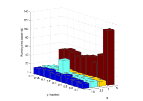
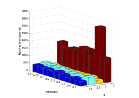
Figure 1: Running times for $\ell_{1,q}$-norm projections as scalars $q$ and ratios $\gamma/\|{V}\|_{1,q}$ vary. The left plot is on a ${1000\times 100}$ matrix, while the right one is on a $5000\times 500$ matrix.

4.3 Application to Multitask Lasso

Multitask Lasso (Mtl) [44, 24] is a simple grouped feature selection problem, which separates important features from less important ones by using information shared across multiple tasks. The feature selection is effected by a sparsity promoting mixed-norm, usually the $\ell_{1,\infty}$-norm [24].

Formally, Mtl is setup as follows. Let $\bm{X}_{j}\in\mathbb{R}^{m_{j}\times d}$ be the data matrix for task $j$, where $1\leq j\leq n$. Mtl seeks a matrix $W\in\mathbb{R}^{d\times n}$, each column of which corresponds to parameters for a task; these parameters are regularized across features by applying a mixed-norm over the rows of $W$. This leads to a “grouped” feature selection, because if for a row, the norm $\|{w^{i}}\|_{\infty}=0$, then the entire row $w^{i}$ gets eliminated (i.e., feature $i$ is removed). The standard Mtl optimization problem is

$$\min_{w_{1},\ldots,w_{n}}\quad\mathcal{L}(W):=\sum\nolimits_{j=1}^{n}\tfrac{1}{2}\|{y_{j}-X_{j}w_{j}}\|_{2}^{2},\quad\text{s.t.}\quad\sum\nolimits_{i=1}^{d}\|{w^{i}}\|_{\infty}\leq\gamma,$$ (4.3)

where the $y_{j}$ are the dependent variables, and $\gamma>0$ is a sparsity-tuning parameter. Notice that the loss-function combines the different tasks (over columns of $W$), but the overall problem does not decompose into separable problems because the mixed-norm constrained is over the rows of $W$.

4.3.1 Stochastic-gradient based MTL

We may rewrite the MTL problem as

$$\begin{split}\min\ L(W):=&\sum\nolimits_{j=1}^{n}\tfrac{1}{2}\|{y_{j}-X_{j}w_{j}}\|_{2}^{2}=\tfrac{1}{2}\|{y-Xw}\|_{2}^{2},\\ \text{s.t.}\quad&\sum\nolimits_{i=1}^{d}\|{w^{i}}\|_{\infty}\leq\gamma,\end{split}$$ (4.4)

where we have introduced the notation

$$y=\operatorname{vec}(Y),\quad X=X_{1}\oplus\cdots\oplus X_{n},\quad\text{and}\ w=\operatorname{vec}(W),$$

in which $\operatorname{vec}(\cdot)$ is the operator that stacks columns of its argument to yield a long vector, and $\oplus$ denotes the direct sum of two matrices. Notice that if it were not for the $\ell_{1,\infty}$-norm constraint, problem (4.4) would just reduce to ordinary least squares.

The form (4.4), however, makes it apparent how to derive a stochastic-gradient method. In particular, suppose that we use a “mini-batch” of size $b$, i.e., we choose $b$ rows of matrix $X$, say $X_{b}$. Let $y_{b}$ denote the corresponding rows (components) of $y$. This subset of rows contributes $\ell_{b}(w):=\tfrac{1}{2}\|{y_{b}-X_{b}w}\|_{2}^{2}$ to the objective (4.4), whereby we have the stochastic-gradient

$$\nabla\ell_{b}(w)=X_{b}^{T}(X_{b}w-y_{b}).$$ (4.5)

Then, upon instantiating iteration (3.4) with (4.5), we obtain Algorithm 2.

Input: Scalar $\gamma>0$; batchsize $b$; stepsize sequence: $\eta_{0},\eta_{1},\ldots$

Output: $W^{*}\approx\operatorname*{argmin}_{W}\ L(W)$, s.t. $\|{W^{T}}\|_{1,\infty}\leq\gamma$

$W_{0}\leftarrow 0$;

while $\neg$ converged do

       Pick $b$ different indices in $[mn]$;

       Obtain stochastic gradient using (4.5);

       $W_{t}\leftarrow\text{proj}(W_{t-1}-\eta_{t}\nabla\ell_{s}(W_{t}))$;

       $t\leftarrow t+1$;

      

return $W^{*}$

Algorithm 2 MTL via stochastic-gradient descent

Implementation notes:

Despite our careful implementation, for large-scale problems the projection can become the bottleneck in Algorithm 2. To counter this, we should perform projections only occasionally—the convergence analysis is unimpeded, as we may restrict our attention to the subsequence of iterates for which projection was performed. Other implementation choices such as size of the mini-batch and the values of the stepsizes $\eta_{t}$ are best determined empirically. Although tuning $\eta_{t}$ can be difficult, this drawback is offset by the gain in scalability.

4.3.2 Simulation results

We illustrate running time results of SPG on two large-scale instances of Mtl (see Table 4). We report running time comparisons between two different invocations of an SPG-based method for solving (4.3), once with QP as the projection method and once with FP—we call the corresponding solvers SPG${}_{\text{QP}}$, and SPG${}_{\text{FP}}$. We note in passing that other efficient Mtl algorithms (e.g., [20, 26]) solve the penalized version; our formulation is constrained, so we only show SPG.

Name	$(m,d,n)$	#nonzeros
D1	(1K, 5K, 10K)	50 million
D2	(10K, 50K, 1K)	500 million

Table 4: Sparse datasets used for MTL. For simplicity, all matrices $X_{j}$ (for each task $1\leq j\leq n$), were chosen to have the same size ${m\times d}$.

Dataset	#projs	proj${}_{\text{QP}}$	proj${}_{\text{FP}}$	SPG${}_{\text{QP}}$	SPG${}_{\text{FP}}$
D1	50	2275.2s	1204.3s	2722.9s	1728.3s
D2	48	2631.8s	1362.3s	3495.1s	2296.7s

Table 5: Running times (seconds) on datasets D1 and D2. SPG was used to solve MTL, with stopping tolerance of $10^{-5}$. Total number of projections required to reach this accuracy are reported as ’#projs’. The columns ’proj${}_{\text{QP}}$’ and ’proj${}_{\text{FP}}$’, report the total time spent by the SPG${}_{\text{QP}}$ and SPG${}_{\text{FP}}$ methods for the $\ell_{1,\infty}$-projections alone. The last two columns report the overall time taken by SPG${}_{\text{QP}}$ and SPG${}_{\text{FP}}$.

The results in Table 4 indicate that for large-scale problems, the savings accrued upon using our faster projections (in combination with SPG) can be substantial.

4.3.3 MTL results on real-world data

We now show a running comparison between three methods: (i) SPG${}_{\text{QP}}$, (ii) SPG${}_{\text{FP}}$, and (iii) SGD (with projection step computed using FP). For our comparison, we solve Mtl on a subset of the CMU Newsgroups dataset.

The dataset corresponds to 5 feature selection tasks based on data taken from the following newsgroups: computer, politics, science, recreation, and religion. The feature selection tasks are spread over the matrices $\bm{X}_{1},\ldots,\bm{X}_{5}$, each of size $2907\times 53975$, while the dependent variables $\bm{y}_{1},\ldots,\bm{y}_{5}$ correspond to class labels.

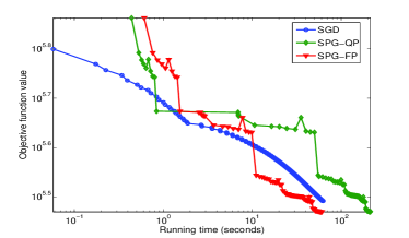
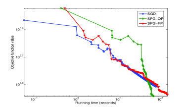
Figure 2: Running time results on CMU Newsgroups subset (left: less sparse; right: more sparse problem).

Figure 2 reports running time results obtained by the three methods in question (all methods were initialized by the same $W_{0}$). As expected, the stochastic-gradient based method rapidly achieves a low-accuracy solution, but start slowing down as time proceeds, and eventually gets overtaken by the SPG based methods. Interestingly, in the first experiment, SPG${}_{\text{QP}}$ takes much longer than SPG${}_{\text{FP}}$ to convergence, while in the second experiment, it lags behind substantially before accelerating towards the end. We attribute this difference to the difficulty of the projection subproblem: in the beginning, the sparsity pattern has not yet emerged, which drives SPG${}_{\text{QP}}$ to take more time. In general, however, from the figure it seems that either SGD or SPG${}_{\text{FP}}$ yield an approximate solution more rapidly—so for problems of increasingly larger size, we might prefer them.

5 Discussion

We described mixed-norms for vectors, which we then naturally extended also to matrices. We presented some duality theory, which enabled us to derive root-finding algorithms for efficiently computing projections onto mixed-norm balls, especially for the special class of $\ell_{1,q}$-mixed norms. For solving an overall regression problem involving mixed-norms we suggested two main algorithms, spectral projected gradient and stochastic-gradient (for separable losses). We presented a small but indicative set of experiments to illustrate the computational benefits of our ideas, in particular for the multitask lasso problem.

At this point, several directions of future work remain open—for instance:

• Designing fast projection methods for certain classes of non-separable mixed norms. Some algorithms already exist for particular classes [1, 28].

• Studying norm projections with additional simple constraints (e.g., bounds).

• Extending the fast methods of this paper to non-Euclidean proximity operators.

• Exploring applications of matrix mixed-norm regularizers.

References

- [1] Bach, F.: Structured sparsity-inducing norms through submodular functions. In: NIPS (2010)
- [2] Bach, F., Jenatton, R., Mairal, J., Obozinski, G.: Convex optimization with sparsity-inducing norms. In: S. Sra, S. Nowozin, S.J. Wright (eds.) Optimization for Machine Learning. MIT Press (2011)
- [3] Bach, F.R.: Consistency of the Group Lasso and Multiple Kernel Learning. J. Mach. Learn. Res. 9, 1179–1225 (2008)
- [4] Barzilai, J., Borwein, J.M.: Two-Point Step Size Gradient Methods. IMA Journal of Numerical Analysis 8(1), 141–148 (1988)
- [5] van den Berg, E., Schmidt, M., Friedlander, M.P., Murphy, K.: Group sparsity via linear-time projection. Tech. Rep. TR-2008-09, Univ. British Columbia (2008)
- [6] Bertsekas, D.P.: Nonlinear Programming, second edn. Athena Scientific (1999)
- [7] Bhatia, R.: Matrix Analysis. Springer (1997)
- [8] Birgin, E.G., Martínez, J.M., Raydan, M.: Nonmonotone Spectral Projected Gradient Methods on Convex Sets. SIAM J. Opt. 10(4), 1196–1211 (2000)
- [9] Birgin, E.G., Martínez, J.M., Raydan, M.: Inexact Spectral Projected Gradient Methods on Convex Sets. IMA Journal of Numerical Analysis 23, 539–559 (2003)
- [10] Cai, J.F., Candes, E.J., Shen, Z.: A Singular Value Thresholding Algorithm for Matrix Completion. SIAM Journal on Optimization 20(4), 1956–1982 (2010)
- [11] Combettes, P.L., Pesquet, J.: Proximal Splitting Methods in Signal Processing. arXiv:0912.3522v4 (2010)
- [12] Dai, Y.H., Fletcher, R.: Projected Barzilai-Borwein Methods for Large-scale Box-constrained Quadratic Programming. Numerische Mathematik 100(1), 21–47 (2005)
- [13] Donoho, D.: Denoising by soft-thresholding. IEEE Tran. Inf. Theory 41(3), 613–627 (2002)
- [14] Duchi, J., Singer, Y.: Online and Batch Learning using Forward-Backward Splitting. JMLR (2009)
- [15] Evgeniou, T., Micchelli, C., Pontil, M.: Learning multiple tasks with kernel methods. J. Mach. Learn. Res. 6, 615–637 (2005)
- [16] Evgeniou, T., Pontil, M.: Regularized multi-task learning. In: KDD (2004)
- [17] Friedman, J., Hastie, T., Tibshirani, R.: A note on the group lasso and a sparse group lasso. arXiv:1001.0736v1 [math.ST] (2010)
- [18] Horn, R.A., Johnson, C.R.: Topics in Matrix Analysis. Cambridge University Press, Cambridge (1991)
- [19] Jenatton, R., Mairal, J., Obozinski, G., Bach, F.: Proximal Methods for Sparse Hierarchical Dictionary Learning. In: ICML (2010)
- [20] Kim, D., Sra, S., Dhillon, I.S.: A scalable trust-region algorithm with application to mixed-norm regression. In: Int. Conf. Machine Learning (ICML) (2010)
- [21] Kiwiel, K.: On Linear-Time Algorithms for the Continuous Quadratic Knapsack Problem. Journal of Optimization Theory and Applications 134, 549–554 (2007)
- [22] Kowalski, M.: Sparse regression using mixed norms. Applied and Computational Harmonic Analysis 27(3), 303 – 324 (2009)
- [23] Lewis, A.: The Convex Analysis of Unitarily Invariant Matrix Functions. J. Convex Analysis 2(1), 173–183 (1995)
- [24] Liu, H., Palatucci, M., Zhang, J.: Blockwise Coordinate Descent Procedures for the Multi-task Lasso, with Applications to Neural Semantic Basis Discovery. In: Int. Conf. Machine Learning (2009)
- [25] Liu, J., Ye, J.: Efficient Euclidean projections in linear time. In: ICML (2009)
- [26] Liu, J., Ye, J.: Efficient L1/Lq Norm Regularization. arXiv:1009.4766v1 (2010)
- [27] Liu, J., Ye, J.: Moreau-Yosida Regularization for Grouped Tree Structure Learning. In: NIPS (2010)
- [28] Mairal, J., Jenatton, R., Obozinski, G., Bach, F.: Network Flow Algorithms for Structured Sparsity. In: NIPS (2010)
- [29] Michelot, C.: A finite algorithm for finding the projection of a point onto the canonical simplex of . J. Optim. Theory Appl. 50(1), 195–200 (1986)
- [30] Obonzinski, G., Taskar, B., Jordan, M.: Multi-task feature selection. Tech. rep., UC Berkeley (2006)
- [31] Patriksson, M.: A survey on a classic core problem in operations research. Tech. Rep. 2005:33, Chalmers University of Technology and Göteborg University (2005)
- [32] Polyak, B.T.: Introduction to Optimization. Optimization Software (1987)
- [33] Quattoni, A., Carreras, X., Collins, M., Darrell, T.: An Efficient Projection for Regularization. In: ICML (2009)
- [34] Rakotomamonjy, A., Flamary, R., Gasso, G., Canu, S.: penalty for sparse linear and sparse multiple kernel multi-task learning. Tech. Rep. hal-00509608, Version 1, INSA-Rouen (2010)
- [35] Rice, U.: Compressive sensing resources. http://dsp.rice.edu/cs (2010)
- [36] Rish, I., Grabarnik, G.: Sparse modeling: ICML 2010 tutorial. Online (2010)
- [37] Rockafellar, R.T.: Convex Analysis. Princeton Univ. Press (1970)
- [38] Rosen, J.: The Gradient Projection Method for Nonlinear Programming. Part I. Linear Constraints. Journal of the Society for Industrial and Applied Mathematics 8(1), 181–217 (1960)
- [39] Schmidt, M., van den Berg, E., Friedlander, M., Murphy, K.: Optimizing Costly Functions with Simple Constraints: A Limited-Memory Projected Quasi-Newton Algorithm. In: AISTATS (2009)
- [40] Similä, T., Tikka, J.: Input selection and shrinkage in multiresponse linear regression. Comp. Stat. & Data Analy. 52(1), 406 – 422 (2007)
- [41] Sra, S.: Fast projections onto -norm balls for grouped feature selection. In: European Conf. Machine Learning (ECML) (2011)
- [42] Tomioka, R., Suzuki, T., Sugiyama, M.: Augmented Lagrangian Methods for Learning, Selecting, and Combining Features. In: S. Sra, S. Nowozin, S.J. Wright (eds.) Optimization for Machine Learning. MIT Press (2011)
- [43] Tropp, J.A.: Algorithms for simultaneous sparse approximation, Part II: Convex relaxation. Signal Proc. 86(3), 589–602 (2006)
- [44] Turlach, B.A., Venables, W.N., Wright, S.J.: Simultaneous Variable Selection. Technometrics 27, 349–363 (2005)
- [45] Yuan, M., Lin, Y.: Model Selection and Estimation in Regression with Grouped Variables. Tech. Rep. 1095, Univ. of Wisconsin, Dept. of Stat. (2004)
- [46] Zhang, Y., Yeung, D.Y., Xu, Q.: Probabilistic Multi-Task Feature Selection. In: NIPS (2010)
- [47] Zhao, P., Rocha, G., Yu, B.: The composite absolute penalties family for grouped and hierarchical variable selection. Ann. Stat. 37(6A), 3468–3497 (2009)