D-wave superconductivity induced by short-range antiferromagnetic correlations in the two-dimensional Kondo lattice model

Abstract

The possible heavy fermion superconductivity is carefully reexamined in the two-dimensional Kondo lattice model with an antiferromagnetic Heisenberg superexchange between local magnetic moments. In order to establish an effective mean field theory in the limit of the paramagnetic heavy Fermi liquid and near the half-filling case, we find that the spinon singlet pairing from the local antiferromagnetic short-range correlations can reduce the ground state energy substantially. In the presence of the Kondo screening effect, the Cooper pairs between the conduction electrons is induced. Depending on the ratio of the Heisenberg and the Kondo exchange couplings, the resulting superconducting state is characterized by either a d-wave nodal or d-wave nodeless state, and a continuous phase transition exists between these two states. These results are related to some quasi-two dimensional heary fermion superconductors.

I Introduction

Heavy fermion materials have been playing a particular important role in our understanding of strongly correlated electron systemsStewart ; Lohneysen , and the Kondo lattice model is believed to capture the basic physics of heavy fermion systemsSi-2001 . The model describes a lattice of local spin-1/2 magnetic moments coupled antiferromagnetically to a single band of conduction electrons. When the number of conduction electrons is less than the number of the local magnetic moments, the coherent superposition of individual Kondo screening clouds gives rise to the huge mass enhancement of the quasiparticles, and the resulting metallic state is characterized by a large Fermi surface with the Luttinger volume containing both conduction electrons and local momentsOgata-2007 ; Assaad-2008 . Competing with the Kondo singlet formation, the local magnetic moments indirectly interact with each other via magnetic polarization of the conduction electrons – the Ruderman-Kittel-Kasuya-Yosida (RKKY) interaction. Such an interaction dominates at low values of the Kondo exchange coupling and is the driving force for the antiferromagnetic (AFM) long-range order near the half-filling of the conduction electrons Doniach ; Lacroix-Cyrot ; zhang-2000 .

In addition, there have been growing evidence that the antiferromagnetism is also intimate with superconductivity in some typical heavy fermion compounds, such as CeCu₂Si₂ (Ref.Steglich-1979 ) and CeRhIn₅ (Ref.Parks-2006 ). So far various mechanisms for heavy fermion superconductivity have been studied, including paramagnon exchangeAnderson ; Scalapino , conventional phonon-mediatedFulde , and Kondo-boson-mediated pairingsAuerbach-1986 ; Millis-1986 ; Lavagna . So far the pairing mechanism of the heavy quasiparticles is still under investigation theoretically. However, various experimental evidences in some heavy fermion materials strongly support the d-wave pairing superconductivityThalmeier-Steglich .

It is well established that the large-$N$ fermionic approach can be used to treat the Kondo lattice model very efficiently, leading to a stable paramagnetic heavy Fermi liquid stateread-newns ; Millis-1986 ; Auerbach-1986 . Qualitatively, the RKKY interaction promotes singlet formation among the local magnetic moments, reducing the tendency of singlet formation between the local moments and conduction electrons. To simplify the RKKY interaction, one can explicitly introduce the local AFM Heisenberg superexchange $J_{H}$ among the local moments to the Kondo lattice systemColeman-1989 ; Coqblin-1997 ; Senthil-2004 ; Coleman-2005 ; Pepin-2008 ; Senthil-2009 ; zhang-2011 . Thus, the paramagnetic heavy Fermi liquid state ($J_{K}>J_{H}$) provides a good starting point for theoretical considerations, because a number of instabilities can be further discussed, including the AFM ordered state and unconventional heavy fermion superconductivity. Recently, some numerical evidences on robust d-wave pairing correlations have been given in small size Kondo-Heisenberg lattice systemDagotto .

In this paper, we try to establish an effective mean field (MF) theory to the Kondo-Heisenberg lattice model on a two-dimensional square lattice in the limit of $J_{K}\gg J_{H}$. After carefully examining three different MF treatments for the local AFM Heisenberg superexchange, we find that the spinon or f-fermion pairings can substantially save the ground state energy in the presence of the Kondo screening. Near the half-filling, the Cooper pairs between the conduction electrons can be induced via the Kondo screening effects. We further find that the resulting superconducting pairing function has a d-wave symmetry. Whether there are nodes or not depends on the ratio of the local AFM Heisenberg and the Kondo exchange couplings $x=J_{H}/J_{K}$. There is a continuous phase transition between the nodal and nodeless superconducting phases. Before the magnetic phase transition, the Kondo screening order parameter is strongly suppressed, and the present mean field theory is no longer valid.

II Mean field treatment

The model Hamiltonian of the Kondo-Heisenberg lattice model is given by:

$$H=\sum_{\mathbf{k},\sigma}\epsilon_{\mathbf{k}}c_{\mathbf{k}\sigma}^{\dagger}c_{\mathbf{k}\sigma}+J_{K}\sum_{i}\mathbf{S}_{i}\cdot\mathbf{s}_{i}+J_{H}\sum_{\left\langle ij\right\rangle}\mathbf{S}_{i}\cdot\mathbf{S}_{j},$$ (1)

where $c_{k\sigma}^{\dagger}$ creates a conduction electron on an extended orbital with wave vector $\mathbf{k}$ and z-component of spin $\sigma=\uparrow,\downarrow$. The spin-1/2 operators of the local magnetic moments have the fermionic representation $\mathbf{S}_{i}=\frac{1}{2}\sum_{\sigma\sigma^{\prime}}f_{i\sigma}^{\dagger}\mathbf{\tau}_{\sigma\sigma^{\prime}}f_{i\sigma^{\prime}}$ where $\mathbf{\tau}$ is the Pauli matrices. There are two local constraints: $\sum_{\sigma}f_{i\sigma}^{\dagger}f_{i\sigma}=1$ and $f_{i\uparrow}f_{i\downarrow}=0$. The former local constraint restricts any charge fluctuations, the f-fermions just describe the spin degrees of freedom of the local moments, and we will refer them to spinons. The latter constraint is imposed by the spin SU(2) symmetry and the extended s-wave spinon pairing between spinons can be excluded. So the paramagnetic Fermi liquid limit ($J_{K}\gg J_{H}$) provides us a good starting point of theoretical considerations.

It is first noticed that the Kondo spin exchange can be expressed as the singlet pairing attraction between the spinon holes and conduction electrons up to a chemical potential shift

$$\mathbf{S}_{i}\cdot\mathbf{s}_{i}=-\frac{1}{2}\left(f_{i\uparrow}^{\dagger}c_{i\uparrow}+f_{i\downarrow}^{\dagger}c_{i\downarrow}\right)\left(c_{i\uparrow}^{\dagger}f_{i\uparrow}+c_{i\downarrow}^{\dagger}f_{i\downarrow}\right).$$ (2)

Then the Kondo screening order parameters can be introduced as

$$V=\left\langle f_{i\uparrow}^{\dagger}c_{i\uparrow}+f_{i\downarrow}^{\dagger}c_{i\downarrow}\right\rangle.$$ (3)

For the non-magnetic states, the local AFM Heisenberg superexchange can be expressed in terms of either the spinon hopping or singlet pairing operators

$$\mathbf{S}_{i}\cdot\mathbf{S}_{j} =-\frac{1}{2}(f_{i\uparrow}^{\dagger}f_{j\uparrow}+f_{i\downarrow}^{\dagger}f_{j\downarrow})(f_{j\uparrow}^{\dagger}f_{i\uparrow}+f_{j\downarrow}^{\dagger}f_{i\downarrow})+\frac{1}{4}$$

$$=-\frac{1}{2}(f_{i{\uparrow}}^{{\dagger}}f_{j\downarrow}^{{\dagger}}-f_{i\downarrow}^{{\dagger}}f_{j{\uparrow}}^{{\dagger}})({{f}_{j\downarrow}{f}_{i{\uparrow}}-{f}_{j{\uparrow}}{f}_{i\downarrow})+}\frac{1}{4}.$$ (4)

However, most of previous theoretical studies on the Kondo-Heisenberg lattice modelCoqblin-1997 ; Senthil-2004 ; Coleman-2005 ; Pepin-2008 ; Senthil-2009 ; zhang-2011 , only introduced the spinon hopping order parameter. Actually, Coleman and AndreiColeman-1989 had emphasized that the local SU(2) gauge invariance of the local Heisenberg spin operator generally requires the consideration of both MF order parameters. Moreover, recent advances in this area have been made by using symplectic representation of the local magnetic spins Coleman-2010 . Here we first introduce two MF valence bond order parameters to characterize the short-range AFM correlations between the local moments

$$\chi_{ij}=-\langle f_{i\uparrow}^{\dagger}f_{j\uparrow}+f_{i\downarrow}^{\dagger}f_{j\downarrow}\rangle,\Delta_{ij}=-\langle f_{i{\uparrow}}^{{\dagger}}f_{j\downarrow}^{{\dagger}}-f_{i\downarrow}^{{\dagger}}f_{j{\uparrow}}^{{\dagger}}\rangle.$$ (5)

To avoid the incidental degeneracy of the conduction electron band on a square lattice, we choose $\epsilon_{\mathbf{k}}=-2t\left(\cos k_{x}+\cos k_{y}\right)+4t^{\prime}\cos k_{x}\cos k_{y}-\mu$, where $t$ and $t^{\prime}$ are the first and second nearest neighbor hoping matrix elements, while $\mu$ is the chemical potential, which should be determined self-consistently by the density of conduction electrons $n_{c}$. When the local AFM correlation hopping parameter $\chi$ is simply chosen as a uniform parameter, the spinons form a very narrow band with a dispersion $\chi_{\mathbf{k}}=J_{H}\chi(\cos k_{x}+\cos k_{y})+\lambda$, where $\lambda$ is the Lagrangian multiplier to impose the local constraint $\sum_{\sigma}f_{i\sigma}^{\dagger}f_{i\sigma}=1$ on average. For the short-range AFM spinon singlet pairing order parameter $\Delta_{ij}$, the local pairing constraint $f_{i\uparrow}f_{i\downarrow}=0$ excludes the extended s-wave pairing, and then d-wave symmetric pairings lead to a lower ground state energyKotliar-Liu , corresponding to $\Delta_{i,i+e_{x}}=-\Delta_{i,i+e_{y}}\equiv\Delta_{0}$.

Then the MF model Hamiltonian in momentum space can be written as

$$H{{}_{mf}} =\sum_{\mathbf{k}\sigma}\varepsilon_{\mathbf{k}}c_{\mathbf{k}\sigma}^{{\dagger}}c_{\mathbf{k}\sigma}-\frac{J_{K}V}{2}\sum_{\mathbf{k}\sigma}\left(f_{\mathbf{k}\sigma}^{{\dagger}}c_{\mathbf{k}\sigma}+c_{\mathbf{k}\sigma}^{{\dagger}}f_{\mathbf{k}\sigma}\right)$$

$$\text{ \ \ }+J_{H}\sum_{\mathbf{k}}\Delta(\mathbf{k})(f_{\mathbf{k}{\uparrow}}^{{\dagger}}f_{-\mathbf{k}\downarrow}^{{\dagger}}+h.c.)+N\epsilon_{0}$$

$$\text{ \ \ }+\sum_{\mathbf{k}\sigma}\chi_{\mathbf{k}}f_{\mathbf{k}\sigma}^{{\dagger}}f_{\mathbf{k}\sigma},$$ (6)

where $\Delta_{\mathbf{k}}\equiv\Delta_{\mathbf{0}}(\cos k_{x}-\cos k_{y})$ and $\epsilon_{0}=(\frac{J_{K}V^{2}}{2}+J_{H}\Delta_{0}^{2}+J_{H}\chi^{2}-\lambda)$. When a Nambu spinor is defined by $\psi_{\mathbf{k}}^{\dagger}=\left(\begin{array}[]{cccc}c_{\mathbf{k}\uparrow}^{{\dagger}}&c_{-\mathbf{k}\downarrow}&f_{\mathbf{k}\uparrow}^{{\dagger}}&f_{-\mathbf{k}\downarrow}\end{array}\right)$, we can express the MF model Hamiltonian in a matrix form

$$H{{}_{mf}} =\sum_{\mathbf{k}}\psi_{\mathbf{k}}^{\dagger}\left(\begin{array}[]{cccc}\varepsilon_{\mathbf{k}}&0&-\frac{J_{K}V}{2}&0\\ 0&-\varepsilon_{\mathbf{k}}&0&\frac{J_{K}V}{2}\\ -\frac{J_{K}V}{2}&0&\chi_{\mathbf{k}}&J_{H}\Delta_{\mathbf{k}}\\ 0&\frac{J_{K}V}{2}&J_{H}\Delta_{\mathbf{k}}&-\chi_{\mathbf{k}}\end{array}\right)\psi_{\mathbf{k}}$$ (11)

$$\text{ \ \ \ \ }+\sum_{\mathbf{k}}\left(\varepsilon_{\mathbf{k}}+\chi_{\mathbf{k}}\right)+N\epsilon_{0},$$ (12)

Diagonalizing this MF model Hamiltonian, we obtain two quasiparticle energy bands

$$E_{\mathbf{k}}^{\pm}\equiv\sqrt{E_{\mathbf{k}1}\pm\sqrt{E_{\mathbf{k}1}^{2}-E_{\mathbf{k}2}^{2}}},$$ (13)

where

$$E_{\mathbf{k}1} \equiv\frac{1}{2}\left(\varepsilon_{\mathbf{k}}^{2}+\chi_{\mathbf{k}}^{2}+J_{H}^{2}\Delta_{\mathbf{k}}^{2}\right)+\frac{1}{4}(J_{K}V)^{2},$$

$$E_{\mathbf{k}2} \equiv\sqrt{(\varepsilon_{\mathbf{k}}\chi_{\mathbf{k}}-\frac{J_{K}^{2}V^{2}}{4})^{2}+(\varepsilon_{\mathbf{k}}J_{H}\Delta_{\mathbf{k}})^{2}}.$$ (14)

Due to the particle-hole symmetry of the superconducting quasiparticles, all the negative energy states are filled up at zero temperature, and the ground state energy per site is thus given by

$$E_{g}=\frac{1}{N}\sum_{\mathbf{k}}\left(\varepsilon_{\mathbf{k}}-E_{\mathbf{k}}\right)+\frac{J_{K}V^{2}}{2}+J_{H}\left(\Delta_{0}^{2}+\chi^{2}\right),$$ (15)

where $E_{\mathbf{k}}\equiv E_{\mathbf{k}}^{+}+E_{\mathbf{k}}^{-}=\sqrt{2E_{\mathbf{k}1}+2E_{\mathbf{k}2}}$. The saddle point equations for the MF order parameters $V$, $\chi$, $\Delta_{0}$ and $\lambda$ can be determined by minimizing the ground state energy:

$$\frac{\partial E_{g}}{\partial V}=\frac{\partial E_{g}}{\partial\chi}=\frac{\partial E_{g}}{\partial\lambda}=\frac{\partial E_{g}}{\partial\Delta_{0}}=0.$$ (16)

The chemical potential $\mu_{c}$ is determined by the relation $n_{c}=-\frac{\partial E_{g}}{\partial\mu_{c}}$. Therefore, the self-consistent equations at zero temperature are given by,

$$\frac{1}{N}\sum_{\mathbf{k}}\frac{1}{E_{\mathbf{k}}}\left[\varepsilon_{\mathbf{k}}+\frac{\chi_{\mathbf{k}}(\varepsilon_{\mathbf{k}}\chi_{\mathbf{k}}-J_{K}^{2}V^{2}/4)+\varepsilon_{\mathbf{k}}J_{H}^{2}\Delta_{\mathbf{k}}^{2}}{E_{\mathbf{k}2}}\right] =\left(1-n_{c}\right),$$

$$\frac{1}{N}\sum_{\mathbf{k}}\frac{1}{E_{\mathbf{k}}}\left[\chi_{\mathbf{k}}+\frac{\varepsilon_{\mathbf{k}}(\varepsilon_{\mathbf{k}}\chi_{\mathbf{k}}-J_{K}^{2}V^{2}/4)}{E_{\mathbf{k}2}}\right] =0,$$

$$\frac{1}{N}\sum_{\mathbf{k}}\frac{1}{E_{\mathbf{k}}}\left[1-\frac{(\varepsilon_{\mathbf{k}}\chi_{\mathbf{k}}-J_{K}^{2}V^{2}/4)}{E_{\mathbf{k}2}}\right] =\frac{2}{J_{K}},$$

$$\frac{1}{N}\sum_{\mathbf{k}}\frac{\Delta_{\mathbf{k}}^{2}}{E_{\mathbf{k}}}\left[1+\frac{\varepsilon_{\mathbf{k}}^{2}}{E_{\mathbf{k}2}}\right] =\frac{2\Delta_{0}^{2}}{J_{H}},$$

$$\frac{1}{N}\sum_{\mathbf{k}}\frac{\left(\chi_{\mathbf{k}}-\lambda\right)}{E_{\mathbf{k}}}\left[\chi_{\mathbf{k}}+\frac{\varepsilon_{\mathbf{k}}(\varepsilon_{\mathbf{k}}\chi_{\mathbf{k}}-J_{K}^{2}V^{2}/4)}{E_{\mathbf{k}2}}\right] =2J_{H}\chi^{2}.$$ (17)

In order to simplify the present treatments, we can have three different MF schemes: (1) $\chi=0$ and $\Delta_{0}\neq 0$; (2) $\chi\neq 0$ and $\Delta_{0}\neq 0$; (3) $\chi\neq 0$ and $\Delta_{0}=0$. Without losing generality, we choose $t^{\prime}/t=0.3$, $n_{c}=0.8$ and fixing $J_{K}/t=2.0$, we have carefully solved the self-consistent equations and compared the ground state energy densities for the three different types of MF schemes. The numerical results are not sensitive to the parameters chosen. The numerical results are displayed in Fig. 1. It is clear that, for $0<J_{H}/t<1.3$, the first type of MF ansatz has a comparatively lower ground state energy. As the local AFM coupling $J_{H}/t$ increases, the ground state energy is almost unchanges, and then decreases gradually as $J_{H}/t$ is further increased. However, the ground state energies for two other MF schemes grow up in the beginning and then blend down after reaching their maximal points. Only when $J_{H}/t>1.34$, the ground state energy of the second MF ansatz starts to become lower than that of the first MF ansatz. In the present paper, we will confine our following discussions to the small local AFM Heisenberg exchange coupling $J_{H}/t<1.34$, so only the first type of MF scheme ($\chi=0$ and $\Delta_{0}\neq 0$) will be used.

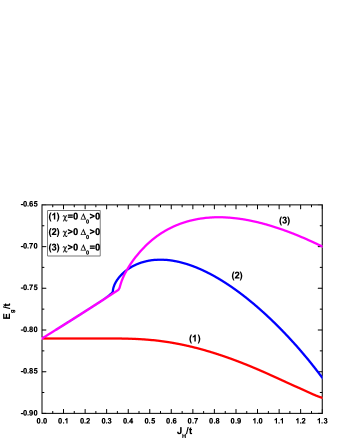
Figure 1: (Color online) The ground state energies of a two-dimensional Kondo-Heisenberg lattice model under three different types of MF approximation schemes for a given value of $J_{K}/t=2.0$. The other parameters are $t^{\prime}/t=0.3$ and $n_{c}=0.8$.

III D-wave superconducting phase

When there is only one short-range AFM correlation order parameters $\Delta_{0}\neq 0$, the MF model Hamiltonian is simplified by

$$H{{}_{mf}^{\prime}} =\sum_{\mathbf{k}\sigma}\varepsilon_{\mathbf{k}}c_{\mathbf{k}\sigma}^{{\dagger}}c_{\mathbf{k}\sigma}-\frac{J_{K}V}{2}\sum_{\mathbf{k}\sigma}\left(f_{\mathbf{k}\sigma}^{{\dagger}}c_{\mathbf{k}\sigma}+c_{\mathbf{k}\sigma}^{{\dagger}}f_{\mathbf{k}\sigma}\right)$$

$$\text{ \ \ }+\lambda\sum_{\mathbf{k}\sigma}f_{\mathbf{k}\sigma}^{{\dagger}}f_{\mathbf{k}\sigma}+J_{H}\sum_{\mathbf{k}}\Delta(\mathbf{k})(f_{\mathbf{k}{\uparrow}}^{{\dagger}}f_{-\mathbf{k}\downarrow}^{{\dagger}}+h.c.)$$

$$\text{ \ \ }+N\left(\frac{J_{K}V^{2}}{2}+J_{H}\Delta_{0}^{2}-\lambda\right),$$ (18)

where the spinons have a flat band. Due to the hybridization effect, the heavy quasiparticle bands form. On the other hand, the spinon singlet pairings imply a special non-magnetic state with short-range AFM correlations among the local magnetic moments. Although there are no any direct attractions among the conduction electrons, the spinon singlet pairings provide an indirect glue for the formation of the Cooper pairs via the Kondo screening/hybridizing effect. So the resulting MF ground state represents a heavy fermion superconducting state.

On a two-dimensional square lattice, the spinon singlet pairing function has a d-wave symmetryKotliar-Liu . Whether there are nodes or not mainly depends on the Lagrangian multiplier $\lambda$ and hybridization strength $V$. From the simplified quasiparticle bands

$$E_{\mathbf{k}}^{\pm} = \sqrt{E_{\mathbf{k},1}\pm\sqrt{E_{\mathbf{k},1}^{2}-E_{\mathbf{k},2}^{2}}},$$

$$E_{\mathbf{k}1} \equiv \frac{1}{2}\left(\varepsilon_{\mathbf{k}}^{2}+\lambda^{2}+J_{H}^{2}\Delta_{\mathbf{k}}^{2}\right)+\frac{1}{4}(J_{K}V)^{2},$$

$$E_{\mathbf{k}2} \equiv \sqrt{(\varepsilon_{\mathbf{k}}\lambda-\frac{J_{K}^{2}V^{2}}{4})^{2}+(\varepsilon_{\mathbf{k}}J_{H}\Delta_{\mathbf{k}})^{2}},$$ (19)

we note that nodes appear in the lower band $E_{\mathbf{k}}^{-}$ when $E_{\mathbf{k},2}=0$, which requires the condition $\varepsilon_{\mathbf{k}}=\frac{J_{K}^{2}V^{2}}{4\lambda}$ in the diagonal direction.

Then the numerical mean field calculations are carefully performed with the parameters $t^{\prime}/t=0.3$, $n_{c}=0.8$ and $J_{K}/t=2.0$. The lower branch of the quasiparticle band $E_{\mathbf{k}}^{-}$ in the first Brillouin zone along the momentum direction ($0,0$)$\rightarrow$($\pi/2,\pi/2$)$\rightarrow$($\pi,\pi$)$\rightarrow$($\pi,\pi/2$)$\rightarrow$($\pi,0$) are plotted in Fig.2 for different local AFM coupling strength $J_{H}/t=0.5$, $0.8$, $1.192$, and $1.3$, respectively. We first notice that the quasiparticle states near the Fermi energy have a very small dispersion, reflecting the quasiparticle mass enhancement in the superconducting state. In Fig.2a and Fig.2b, a node can be clearly seen between the momentum ($\pi/2,\pi/2$) and ($\pi,\pi$) in the diagonal direction. Secondly, the position of the node changes as increasing the local AFM coupling strength. When the nodal position is shifted to ($\pi,\pi$), further increasing $J_{H}/t$ makes a small energy gap open. The critical value can be determined as $J_{H}/t=$ $1.192$. When $1.192<J_{H}/t<1.34$, the resulting superconducting state has a full superconducting gap.

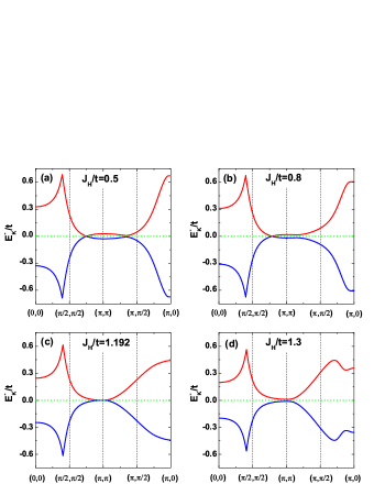
Figure 2: (Color online) The lower branch of the superconducting quasiparticle band struture for different local AFM Heisenberg coupling strength with $t^{\prime}/t=0.3$, $n_{c}=0.8$ and $J_{K}/t=2.0$.

Moreover, the Kondo screening parameter $V$ and the AFM spinon pairing parameter $\Delta_{0}$ have also been calculated, and the numerical results are shown in Fig.3. It can be seen that, as $J_{H}/t$ starts to increase, the Kondo screening parameter is almost unchanged in the beginning and then becomes gradually decreased when $J_{H}/t>0.80$. On the contrary, the spinon pairing order parameter $\Delta_{0}$ is extremely small in the small limit of $J_{H}/t$. Only after $J_{H}/t>0.20$, $\Delta_{0}$ starts to grow up quickly. Actually, we have also plotted a superconducting order parameter $\Delta_{sc}$ defined by the conducting electrons, whose definition will be given later. It should be pointed out that the quantum phase transition mentioned above does not manifest in the MF order parameters.

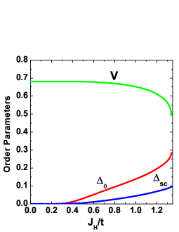
Figure 3: (Color online) The effective mean field order parameters of the Kondo screening $V$, the f-fermion/spinon pairing $\Delta_{0}$, and the Cooper pairing $\Delta_{sc}$ for a given value of $J_{K}/t=2.0$.

As the spinons are paired up in the real lattice space, it is more interesting to display the spinon pairing distribution in the momentum space. Using the method of the equation motion, we can easily derive the double-time retarded Green function for the spinon pairs,

$$\langle\langle f_{-\mathbf{k}\downarrow}^{{\dagger}}|f_{\mathbf{k}\uparrow}^{{\dagger}}\rangle\rangle_{\omega+i0^{+}}=\frac{J_{H}\Delta_{\mathbf{k}}(\omega^{2}-\varepsilon_{k}^{2})}{\left[\omega^{2}-\left(E_{\mathbf{k}}^{+}\right)^{2}\right]\left[\omega^{2}-\left(E_{\mathbf{k}}^{-}\right)^{2}\right]},$$ (20)

from which the expectation value of the spinon pairing function can be evaluated according to the spectral theorem of the Green’s function. At zero temperature, we obtain

$$\left\langle f_{\mathbf{k}\uparrow}^{{\dagger}}f_{-\mathbf{k}\downarrow}^{{\dagger}}\right\rangle=-\frac{J_{H}\Delta_{\mathbf{k}}}{2\sqrt{2\left(E_{\mathbf{k}1}+E_{\mathbf{k}2}\right)}}\left[1+\frac{\varepsilon_{k}^{2}}{E_{\mathbf{k}2}}\right],$$ (21)

which is displayed in Fig.4. When the local AFM coupling strength $J_{H}/t=0.5$, we observe in Fig.4a that the spinon pairing function reflects the d-wave symmetry around the Fermi surface of heavy quasiparticles, which is a hole-like circle around the corner of the first Brillouin zone. A node is clearly seen between the momentum ($\pi/2,\pi/2$) and ($\pi,\pi$) in the diagonal direction. The positive pairing magnitude and the negative pairing magnitude are separated by the nodes. As increasing of $J_{H}/t$, the spinon pairing region is outstretched and the position of the node is shifted toward to ($\pi,\pi$), as shown in Fig.4b. When $J_{H}/t=1.192$, the node starts to disappear, and a small energy gap opens at ($\pi,\pi$).

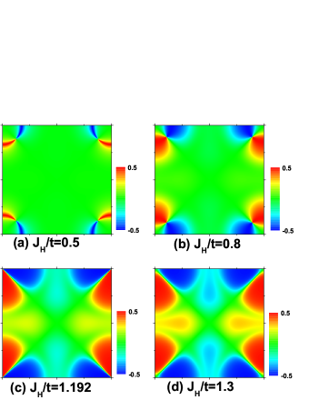
Figure 4: (Color online) The spinon singlet pairing distribution in the first Brillouin zone as increasing local AFM coupling strength for a given value of $J_{K}/t=2.0$..

However, the Cooper pairing function of the conduction electrons is more important for the heavy fermion superconducting state. Similarly, we can easily derive the double-time retarded Green function for the conduction electron pairs

$$\langle\langle c_{-\mathbf{k}\downarrow}^{{\dagger}}|c_{\mathbf{k}\uparrow}^{{\dagger}}\rangle\rangle_{\omega+i0^{+}}=\frac{J_{H}J_{K}^{2}V^{2}\Delta_{\mathbf{k}}}{4\left[\omega^{2}-\left(E_{\mathbf{k}}^{+}\right)^{2}\right]\left[\omega^{2}-\left(E_{\mathbf{k}}^{-}\right)^{2}\right]},$$ (22)

and the superconducting pairing function can be defined from the expectation value of the conduction electron pairs. At zero temperature, we have

$$\left\langle c_{\mathbf{k}\uparrow}^{{\dagger}}c_{-\mathbf{k}\downarrow}^{{\dagger}}\right\rangle=\frac{J_{H}J_{K}^{2}V^{2}\Delta_{\mathbf{k}}}{8E_{\mathbf{k}2}\sqrt{2\left(E_{\mathbf{k}1}+E_{\mathbf{k}2}\right)}},$$ (23)

which has been displayed in Fig.5. When $J_{H}/t=0.5$, we can clearly observe that the positive pairing is distributed around the upper part of the Fermi surface, while the negative pairing is around the lower part of the Fermi surface. Nodes sit in the diagonal directions of the Fermi surface. In contrast to the spinon pairing distribution, there are additional features: a positive electron pairing magnitude is centered around the point ($0,\pi$) and a negative electron pairing magnitude is around the point ($\pi,0$). As the local AFM coupling $J_{H}/t\geq 1.192$, an energy gap opens near the nodes of the Fermi surface, and there are only small pairing distribution on other parts of the Fermi surface. However, the Cooper pairing distributed around momentum ($0,\pi$) and ($\pi,0$) have strong magnitudes. The resulting superconductivity still exhibits the d-wave symmetry, i.e., the d-wave nodeless superconducting state.

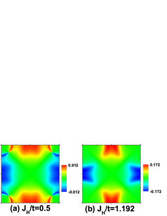
Figure 5: (Color online) The superconducting pairing distribution function in the first Brillouin zone for the local AFM coupling strength $J_{H}/t=0.5$ and $1.192$ with a given value of $J_{K}/t=2.0$.

Moreover, a real superconducting order parameter can be defined by

$$\Delta_{sc}=\frac{1}{2N}\sum_{\mathbf{k}}\left(\cos k_{x}-\cos k_{y}\right)\langle c_{\mathbf{k}\uparrow}^{{\dagger}}c_{-\mathbf{k}\downarrow}^{{\dagger}}+c_{-\mathbf{k}\downarrow}c_{\mathbf{k}\uparrow}\rangle,$$ (24)

which has been displayed in Fig.3. Since it is generated by the spinon singlet pairings, the superconducting order parameter has a smaller magnitude compared to the spinon pairing order parameter $\Delta_{0}$. In order to reveal the quantum phase transition between two superconducting phases, we have to calculate the first order derivative of the ground state energy. For a given value of $J_{K}/t=2.0$, the numerical results are exhibited in Fig.6. At $J_{H}/t=1.192$, the ground state energy and its first derivative are continuous but the second derivative is not. This corresponds the critical point of a second order quantum phase transition.

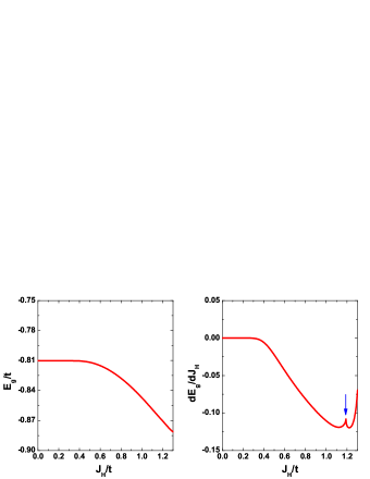
Figure 6: (Color online) The ground state energy density (a) and its first order derivative (b) as a function of $J_{H}/t$ for a given value of $J_{K}/t=2$. The arrow indicates the critical point of quantum phase transition.

IV Discussion and conclusion

So far we have presented the ground state properties of the effective MF theory for the two-dimensional Kondo lattice model with the local AFM Heisenberg exchange coupling between the localized magnetic moments. We would like to emphasize that, it is the local AFM short-range interaction that induces the AFM and superconducting long-range ordering states. When $J_{K}\gg J_{H}$, the local AFM Heisenberg exchange coupling among the local moments is negligible and the stable paramagnetic heavy Fermi liquid state is resulted from the coherent superposition of individual Kondo screening clouds. When $J_{H}$ is increased but still less than $J_{K}$, the local AFM Heisenberg exchange coupling has to be taken into account, and the spinon singlet pairings can reduce the ground state energy significantly. The Cooper singlet pairs among the conduction electrons can be induced via the Kondo screening effect, leading to the heavy fermion superconductivity. This also belongs to the category of the unconventional superconductivity mediated by the short-range AFM correlations. However, in the present MF theory, we do not find a finite critical value of $J_{H}/t$ to separate the heavy fermion liquid and the superconducting phases. This may be caused by the approximation used in the effective MF theory.

The resulting superconducting state exhibits the d-wave symmetry. Whether the Cooper pairing function has nodes or not depends on the ratio of the AFM Heisenberg and Kondo exchange couplings. As the coupling ratio increases, the nodal position is shifted outward along the direction of ($\pi/2,\pi/2$)$\rightarrow$($\pi,\pi$). When the nodal position reaches the end point of the Brillouin zone, a quantum phase transition occurs, and a full superconducting gap is opened at the Fermi energy. As further increasing of $J_{H}/J_{K}$, the present MF theory is no longer valid, because the long-range AFM correlations have to be taken into account.

In conclusion, a possible mechanism of heavy fermion superconductivity with d-wave symmetry is carefully investigated in the two-dimensional Kondo-Heisenberg lattice model from the limit of the paramagnetic heavy Fermi liquid $J_{K}\gg J_{H}$. The resulting d-wave superconducting properties can be related to some heavy fermion superconductors with the similar structure like CeCoIn₅, where thermal conductivity measurements strongly support a superconducting gap with nodes along the diagonal directions in the Brillouin zoneIzawa . Further theoretical work including the estimation of the fluctuations around the MF solution or the coexistent phase of both the AFM order and superconductivity would be necessary to be considered.

The authors would like to thank T. Xiang for stimulating discussions and acknowledge the support of NSF of China and the National Program for Basic Research of MOST-China.

References

- (1) G. Stewart, Rev. Mod. Phys. 73, 797 (2001).
- (2) H. von Lohneysen, A. Rosch, M. Vojta, and P. Wolfle, Rev. Mod. Phys. 79, 1015 (2007).
- (3) Q. Si, S. Rabello, K. Ingersent, and J. Smith, Nature 413, 804 (2001).
- (4) H. Watanabe and M. Ogata, Phys. Rev. Lett. 99, 136401 (2007).
- (5) L. C. Martin and F. F. Assaad, Phys. Rev. Lett. 101, 066404 (2008); L. C. Martin, M. Bercx, and F. F. Assaad, Phys. Rev. B 82, 245105 (2010).
- (6) S. Doniach, Physica B & C 91, 231 (1977).
- (7) C. Lacroix and M. Cyrot, Phys. Rev. B 20, 1969 (1979).
- (8) G. M. Zhang, Q. Gu, and L. Yu, Phys. Rev. B 62, 69 (2000); G. M. Zhang and L. Yu, Phys. Rev. B 62, 67 (2000).
- (9) F. Steglich, et. al., Phys. Rev. Lett. 43, 1892 (1979); H. Q. Yuan, et. al., Science 302, 2104 (2003); O. Stockert, et. al., Nature Physics 7, 119 (2011).
- (10) T. Parks, et. al., Nature 440, 65 (2006); G. Knebel, et. al., Phys. Rev. B 74, 020501 (2006).
- (11) P. W. Anderson, Phys. Rev. B 30, 1549 (1984); K. Miyake, S. Schmitt-Rink, and C. M. Varma, Phys. Rev. B 34, 6554 (1986).
- (12) D. J. Scalapino, E. Loh, and J. E. Hirsch, Phys. Rev. B 34, 8190 (1986).
- (13) H. Razafimandimby, P. Fulde, and J. Keller, Z. Phys. B 54, 111 (1984).
- (14) A. Auerbach and K. Levin, Phys. Rev. Lett. 57, 877 (1986).
- (15) A. J. Millis and P. A. Lee, Phys. Rev. B 35, 3394 (1987).
- (16) M. Lavagna, A. J. Millis, and P. A. Lee, Phys. Rev. Lett. 58, 266 (1987); F. C. Zhang and T. K. Lee, Phys. Rev. B 35, 3651 (1987).
- (17) P. Thalmeier, G. Zwicknagl, O. Stockert, G.Sparn, and F. Steglich, in Frontiers in Superconducting Materials, edited by A. Narlikar, Springer Verlag, Berlin, 2004.
- (18) N. Read and D. M. Newns, J. Phys. C: Solid State Phys. 16, 3273 (1983).
- (19) P. Coleman and N. Andrei, J. Phys.: Condens. Matter 1, 4057 (1989); N. Andrei and P. Coleman, Phys. Rev. Lett. 62, 595 (1989).
- (20) J. R. Iglesias, C. Lacroix, and B. Coqblin, Phys. Rev. B 56, 11820 (1997); B. Coqblin, C. Lacroix, M. S. Gusmao, and J. R. Iglesias, Phys. Rev. B 67, 064417 (2003).
- (21) T. Senthil, M. Vojta, and S. Sachdev, Phys. Rev. B 69, 035111 (2004).
- (22) P. Coleman, J. B. Marston, and A. J. Schofield, Phys. Rev. B 72, 245111 (2005).
- (23) I. Paul, C. Pepin, and M. R. Norman, Phys. Rev. Lett. 98, 026402 (2007); Phys. Rev. B 78, 035109 (2008).
- (24) T. Grover and T. Senthil, Phys. Rev. B 81, 205102 (2010).
- (25) G. M. Zhang, Y. H. Su, and L. Yu, Phys. Rev. B 83,033102 (2011).
- (26) J. C. Xavier and E. Dagotto, Phys. Rev. Lett. 100, 146403 (2008).
- (27) R. Flint, M. Dzero, and P. Coleman, Nature Phys. 4, 643 (2008); R. Flint and P. Coleman, Phys. Rev. Lett. 105, 246404 (2010).
- (28) G. Kotliar and J. Liu, Phys. Rev. B 38, 5142 (1988).
- (29) K. Izawa, H. Yamaguchi, Yuji Matsuda, H. Shishido, R. Settai, and Y. Onuki, Phys. Rev. Lett. 87, 057002 (2001).