D-iteration: application to differential equations

Abstract

In this paper, we study how the D-iteration algorithm can be applied to numerically solve the differential equations such as heat equation in 2D or 3D. The method can be applied on the class of problems that can be addressed by the Gauss-Seidel iteration, based on the linear approximation of the differential equations.

1 Introduction

The iterative methods to solve differential equations based on the linear approximation are very well studied approaches [11], [1], [12], [2], [14], [3], [13]. The approach we propose here (D-iteration) is a new approach initially applied to numerically solve the eigenvector of the Pagerank type equation [8], [7], [6], [4], [5], [10], [9].

The D-iteration, as diffusion based iteration, is an iteration method that can be understood as a column-vector based iteration as opposed to a row-vector based approach. Jacobi and Gauss-Seidel iterations are good examples of row-vector based iteration schemes. While our approach can be associated to the diffusion vision, the existing ones can be associated to the collection vision.

In this paper, we are interested in the numerical solution for linear equation:

$$A.X = B$$ (1)

where $A$ and $B$ are the matrix and vector associated to the linear approximation of differential equations with initial conditions or boundary conditions.

While it is quite clear why diffusion approach is interesting ([7, 10, 9]) when we consider a sparse matrix with a very variable structure of in-degree/out-degree links (non-zero entries of the matrix $A$), the problem statement in the context of linear system associated to differential equation is very different and we try to analyse/explain if there may be an interest to consider a solution such as the D-iteration for those very regular sparse matrix.

2 Example of heat equation

A typical linearized equation of the stationary heat equation in 2D is of the form:

$$T(n,m) =\frac{1}{4}\left(T(n-1,m)+T(n,m-1)\right.$$

$$\qquad\left.+T(n+1,m)+T(n,m+1)\right)$$

which can be obtained by the discretization of the basic equation:

$$\Delta.T(x,y) = \frac{\partial^{2}T}{\partial x^{2}}+\frac{\partial^{2}T}{\partial y^{2}}=0.$$ (2)

inside the surface $\Omega$ (for instance, $\Omega=[0,L_{x}]\times[0,L_{y}]$) Then additive terms appear for the initial or boundary conditions (Dirichlet) on the frontier $\partial\Omega$ (for instance, for $x=0$ or $y=0$ etc).

For this family of equations, the linear dependences remain local (such as averaging of neighbour positions’ values). From the intuitive point of view, the application of iterative methods on such a system is convergent, because the system is diagonally dominant and strictly dominant for the boundary positions, so that the spectral radius of the global system is strictly less than 1. As a consequence, compared to PageRank type equation with a damping factor $d$ for which the spectral radius of the system is explicitly equal to $d<1$ (per row), the convergence of the iterative scheme should be slower for the same size of vector $N$. Indeed, for the linear system we consider here, from the fluid diffusion point of view, instead of having (PageRank equation) a fluid decreasing factor $1-d$ per entry level or vector level iteration, the fluid can only disappear when it reaches the boundary positions (for instance, the positions where the temperature is imposed from a heat source).

Now, in such a context, may the diffusion based iteration scheme be useful, faster? We don’t pretend to give the answer in this paper, we’ll just illustrate the differences and possible advantages through very simple examples.

The D-iteration requires updating two vectors: the fluid vector $F$ and the history vector $H$ instead of a single vector for the Gauss-Seidel. It has been explained that the $H$ vector is the exact connection to the Gauss-Seidel iterations (cf. [10]) when starting from empty initial condition $H_{0}=[0,..,0]$. As it was the case for the iteration on the web graph associated matrix, the utility of $F$ is to give us the exact information on the quantity of fluid that is sent.

Figure 1: Intuition: collection vs diffusion.

Whereas with the web graph, we may wish to apply the diffusion to the node having the maximum amount of fluid (because the fluid that disappears is directly proportional to this quantity), with the matrix we have here, we may wish to find a way to push fluid to the boundary positions as quickly as possible, because inside $\Omega$, the fluid does not disappear.

3 First tests and algorithm adaptation

As a first very simple illustration, we consider the iteration scheme:

$$T(n,m) =\frac{1}{4}\left(T(n-1,m)+T(n,m-1)\right.$$ (3)

$$\qquad\left.+T(n+1,m)+T(n,m+1)\right)$$ (4)

for $n=1,..,L_{x}$ and $m=1,..,L_{y}$ with the boundary condition:

$$T(n,m) =0,\mbox{ if }n=0\mbox{ or }n=L_{x}$$

$$T(n,m) =0,\mbox{ if }m=L_{y}$$

$$T(n,m) =100,\mbox{ if }m=0.$$

We first implemented the Gauss-Seidel iteration using the collection operations defined by:

Collection of (n,m): (averaging)
 T[n][m] :=
    0.25*(T[n-1][m]+T[n][m-1]+T[n+1][m]+T[n][m+1]);

when $(n,m)\notin\partial\Omega$ and the stopping condition:

$$\max_{n,m}|T(n,m)^{k}-T(n,m)^{k-1}|<\epsilon.$$

Then, compared its computation cost to the D-iteration approach with the diffusion condition:

Diffusion of (n,m), if:
 F[n][m] > error;

Remark that if there is no position satisfying $F[n][m]>error$, the condition becomes equivalent to the above stopping condition for Gauss-Seidel iteration.

For $L_{x}=L_{y}=1000$ and an error of $\epsilon=0.1$ (let’s say, we want to know the temperature with a precision of 0.1 degree; one should be careful that the stopping condition defined on the norm $\max$ $L_{\max}$ does not guarantee that the obtained result is effectively at distance $\epsilon$ to the limit), we found the results:

• Gauss-Seidel (GS): 2.35057e+08 operations of collections (over 236 cycles) in 8.3 seconds;

• D-iteration (DI): 2.61681e+06 operations of diffusions (over 629 cycles) in 5.4 seconds.

Diffusion of (n,m):
 received := F[n][m]/4;
 T[n-1][m] += received;
 T[n][m-1] += received;
 T[n+1][m] += received;
 T[n][m+1] += received;

In this case, the boundary condition is such that the heat diffusion is progressive toward the position $y=L_{y}$. Observe that with D-iteration, we did much less operations (by factor 100!), but this implied the diffusion condition tests done on more cycles (629) than for Gauss-Seidel (236 cycles).

To reduce the diffusion condition test cost, we modified the diffusion condition (DC) as:

DC:
Diffusion of (n,m), if:
 F[n][m] > error/delta;

The results when varying $\delta$ is shown in Table 1: we see a clear deterministic effect of $\delta$ when $\delta$ is a multiple of 4 (due to the factor 1/4 of the matrix). 4 seems to be here the optimal value.

$\delta$	cycles	diffusions	time
1	629	2.61681e+06	5.4
2	317	6.65764e+06	3.2
3	232	6.07378e+06	6.1
4	234	6.56046e+06	2.5
5	235	6.89453e+06	6.2
6	235	7.11393e+06	6.2
7	235	7.30539e+06	6.2
8	235	7.45865e+06	2.5
16	236	8.2354e+06	2.5

Table 1: Impact of $\delta$ on the computation cost.

If our understanding is correct, we should have more gain when $L_{y}$ is increased (more stable value): as expected, this is confirmed in Table 2.

$L_{y}$	GS		DI
	collections	time	diffusions	time
1000	2.3e+08	8.25	6.5e+06	2.47
2000	4.7e+08	12.68	6.5e+06	4.79
3000	7.0e+08	15.68	6.5e+06	7.14
4000	9.4e+08	18.76	6.5e+06	9.42
5000	1.1e+09	21.71	6.5e+06	11.77

Table 2: Impact of $L_{y}$ on the computation cost.

While the number of diffusions stays constant for DI, for GS the number of collection operations increases proportionally to $L_{y}$. The increase of the run time with DI is only due to the diffusion condition to be tested on a larger set of points.

With this DC modification, we select the fluid diffusion only at positions where the variation is worth to apply diffusion: when diffusion is applied at position $(n,m)$, $F[n][m]$ is exactly the value by which $H[n][m]$ is increased. With the averaging computation, we are likely to do a lot of useless computations in case certain points of space have converged under the desired precision. And testing this condition would imply the same cost than applying the collection operation (because this would require the knowledge of the variation of the values of neighbour positions): this condition test is exactly what we may do efficiently with $F$.

Here, we observe that the cost of testing diffusion condition (DC) is very important compared to the diffusion cost (see the collections/diffusions ratio compared to the runtime ratio). This is the main difference with the web graph: with web graphs (iterators required for diffusions or collections), the dominant computation cost was the access time to the entries of the matrix with the iterators. Here, this is no more the dominant cost. Therefore, we need a specific optimization to reduce the DC tests.

In order to reduce the diffusion condition test cost, we introduced a new (bool) state variable open:

bool open[n_x][n_y];

which is set to true initially. Then, this state variable is updated as follows:

• when (DC) is not true, we set its open state to false;

• when an open position sends fluids to its neighbour positions, these neighbour positions are set to true.

Then, we test this state value before testing the diffusion condition DC. The results obtained by this modification is illustrate in Table 3.

$L_{y}$	GS		DI
	collections	time	diffusions	time
25	4.3e+06	0.07	4.0e+06	0.11
no op		0.3		0.44
50	1.1e+07	0.16	6.6e+06	0.2
no op		0.74		0.76
100	2.3e+07	0.34	6.6e+06	0.27
no op		1.5		0.86
1000	2.3e+08	8.25	6.6e+06	1.23
no op		21		2.3
2000	4.7e+08	12.68	6.6e+06	2.23
no op		37		3.9
3000	7.0e+08	15.68	6.6e+06	3.22
no op		51		5.5
4000	9.4e+08	18.76	6.6e+06	4.23
no op		66		7.0
5000	1.1e+09	21.71	6.6e+06	5.21
no op		82		8.6

Table 3: Speeding-up the DC test. GS: 236 cycles, DI: 234 cycles (except for $L_{y}=25$: 193, 193). no op: without compiler optimization (option $-O2$ with $g++$).

We see that there is a significant gain on the runtime. Finally, with the adaptation of DC and the introduction of open state variables, the D-iteration may be an interesting candidate to efficiently solve numerically the differential equations.

4 Cost analysis

4.1 Cost decomposition

In order to further understand the performance improvement and the computation cost structure, we introduce the following assumption: we assume that the runtime $RT$ of the solution computation is of the form:

$$RT=(\alpha+\beta)\times(L_{x}\times L_{y})\times\mbox{nb\_iter}+c,$$

where $\alpha$ is the unitary computation cost of one cycle iteration, $\beta$ the average computation cost for one diffusion or one collection, $c$ a constant cost and nb_iter the number of iterations of the cycles.

To estimate the $\alpha$, $\beta$, $c$ values, we first iterated on $x$, $y$ without the collection operations:

sum = 0.0;
counter = 0;
while ( counter < nb_iter ){
  counter++;
  for (int x=0; x < L_x; x++){
    for (int y=0; y < L_y; y++){
      if ( !is_boundary(x,y) )
        sum += T[x][y];
    }
  }
}

where is_boundary(x,y) is a variable (bool) that return true if we are on the position with boundary conditions (or outside $\Omega$). Then $\alpha$ is estimated by dividing the runtime by nb_iter and $L_{x}\times L_{y}$. For $\beta$, we introduce collection operations and then $\alpha+\beta$ is estimated by dividing the runtime by nb_iter and $L_{x}\times L_{y}$.

Finally, $c$ is approximated by the initialization time. For DI, we do the same evaluation with:

sum = 0.0;
counter = 0;
while ( counter < nb_iter ){
  counter++;
  for (int x=0; x < L_x; x++){
    for (int y=0; y < L_y; y++){
      if ( !is_boundary(x,y) and open[x][y] ){
        transit = F[x][y];
        if ( transit > error/scale ){
          sum += T[x][y];
        }
      }
    }
  }
}

adding the DC test for $\alpha$ and then adding the diffusion operations to estimate $\alpha+\beta$. The results are shown on Table 4.

$L_{x}\times L_{y}$	GS		DI
	$\alpha$	$\alpha+\beta$	$\alpha$	$\alpha+\beta$
$100\times 100$	2.0e-08	6.2e-08	3.3e-08	1.0e-07
$200\times 200$	2.0e-08	6.1e-08	3.3e-08	1.0e-07
$1000\times 1000$	2.0e-08	6.7e-08	3.3e-08	1.0e-07
$100\times 1000$	2.0e-08	6.4e-08	3.3e-08	1.0e-07
$200\times 5000$	2.0e-08	6.8e-08	3.4e-08	1.0e-07
$5000\times 200$	2.2e-08	6.3e-08	3.4e-08	1.0e-07

Table 4: Computation cost. Without compiler optimization.

We see that $\alpha$ and $\beta$ are quite stable. We see that the collection cost is roughly 2-3 times the iteration cost for GS (we observed this factor is the one that varies the most with nb_iter). For DI, its iteration cost is more than 1.5 times the iteration cost for GS and the diffusion cost is about 2 times the iteration cost (very stable with nb_iter).

The runtime for GS in Table 3 for $1000\times 1000$ (no op) can be decomposed as 5s (iterations) $+$ 15s (collections). In this case, DI converged with about same number of cycles but with 30 times less diffusions (than collections). So based on the above model, we would have a runtime of: 7.5s for iterations and $15/30\times 2=1$s. But we observed 2.3s instead of 8.5s because most of time we don’t need to test twice the boundary and open condition. We observed that only testing open condition is close (in this case) to the cost to test the boundary condition, but also the main difference comes from the fact that when the open condition is not true, we don’t have to do any computation and this had in this case an impact of cost reduction by up to 3-4 (the iteration runtime for all values $open[x][y]$ set to false runs 3-4 times faster). Therefore, the computation time obtained for DI would be: $5/4+1$.

Now, we could optimize a bit more the DC condition and the boundary position tests including the boundary position information in the state variable open (for instance using, 3 states variable: 0 for boundary position, 1 for not open to DC test, 2 for open to DC test). Results are shown in Table 5.

$L_{y}$	GS		DI
	collections	time	diffusions	time
50	1.1e+07	0.16	6.6e+06	0.18
100	2.3e+07	0.34	6.6e+06	0.26
1000	2.3e+08	8.25	6.6e+06	1.13
2000	4.7e+08	12.68	6.6e+06	2.01
3000	7.0e+08	15.68	6.6e+06	2.89
4000	9.4e+08	18.76	6.6e+06	3.77
5000	1.1e+09	21.71	6.6e+06	4.68

Table 5: Speeding-up the DC test. GS: 236 cycles, DI: 234 cycles.

4.2 The number of diffusions per position

Figure 2 shows the number of diffusions applied per position $y$. We see that above $y=41$, the diffusion is no more applied, whereas with GS, the collection operations need to be applied on all $y$ positions at each cycle.

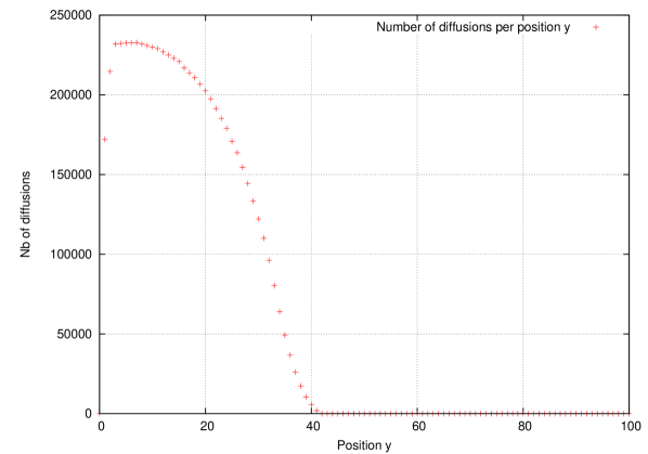
Figure 2: Nb of diffusions applied: per y position.

This example is of course for illustration of a situation when all positions does not converge to the limit at the same speed. If $L_{y}$ is closer to 41, there is no more gain using DC, because all positions are converging almost at the same speed.

Figure 3 shows the number of diffusions per position $y$ when in the case $L_{y}=1000$ we added 10 random positions where $T$ is imposed ($T$ set to a random value between 0 and 1000): in this case, we obtained:

• GS: 697 cycles with 6.94e+08 collections for runtime of 9.5s;

• DI: 687 cycles with 3.97e+07 diffusions for runtime of 4.0s.

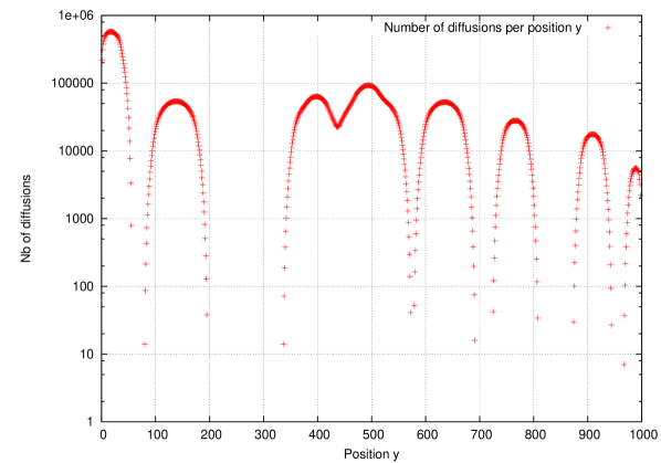
Figure 3: Nb of diffusions applied: per y position: adding 10 random boundary conditions inside $\Omega$.

Figure 4 is an illustration of the limit for the boundary conditions of: $T=100$ on the frontier and $T=0$ imposed at 10 random positions.

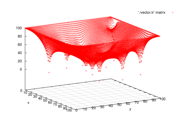
Figure 4: Nb of diffusions applied: $T=100$ on the frontier of $\Omega$ and with 10 random ’holes’ $T=0$.

5 Conclusion

In this paper we addressed a first analysis of the potential of the D-iteration when applied in the context of the numerical solving of differential equations. We showed that this context requires an adaptation of the D-iteration’s fluid diffusion condition. The results are quite promising and we hope to investigate further this application case in the future.

References

- [1] U. M. Ascher and L. R. Petzold. Computer Methods for Ordinary Differential Equations and Differential-Algebraic Equations. Society for Industrial and Applied Mathematics, Philadelphia, PA, USA, 1st edition, 1998.
- [2] C. W. Gear. Numerical Initial Value Problems in Ordinary Differential Equations. Prentice Hall PTR, Upper Saddle River, NJ, USA, 1971.
- [3] G. H. Golub and C. F. V. Loan. Matrix Computations. The Johns Hopkins University Press, 3rd edition, 1996.
- [4] D. Hong. D-iteration based asynchronous distributed computation. arXiv, http://arxiv.org/abs/1202.3108, February 2012.
- [5] D. Hong. D-iteration: Evaluation of a dynamic partition strategy. arXiv, http://arxiv.org/abs/1203.1715, March 2012.
- [6] D. Hong. D-iteration: Evaluation of the asynchronous distributed computation. submitted, http://arxiv.org/abs/1202.6168, February 2012.
- [7] D. Hong. D-iteration method or how to improve gauss-seidel method. arXiv, http://arxiv.org/abs/1202.1163, February 2012.
- [8] D. Hong. Optimized on-line computation of pagerank algorithm. submitted, http://arxiv.org/abs/1202.6158, 2012.
- [9] D. Hong. Revisiting the d-iteration method: computation cost comparisont. arXiv, http://arxiv.org/abs/, March 2012.
- [10] D. Hong. Revisiting the d-iteration method: from theoretical to practical computation cost. arXiv, http://arxiv.org/abs/1203.6030, March 2012.
- [11] C. Johnson. Numerical solution of partial differential equations by the finite element method, volume 32. Cambridge University Press, 1987.
- [12] I. Podlubny. Fractional differential equations: an introduction to fractional derivatives, fractional differential equations, to methods of their solution and some of their applications. Mathematics in Science and Engineering. Academic Press, London, 1999.
- [13] Y. Saad. Iterative Methods for Sparse Linear Systems. Society for Industrial and Applied Mathematics, Philadelphia, PA, USA, 2nd edition, 2003.
- [14] G. D. Smith. Numerical Solution of Partial Differential Equations: Finite Difference Methods, volume 22. Oxford University Press, 1985.