Modulated reheating by curvaton

Abstract

There might be a light scalar field during inflation which is not responsible for the accelerating inflationary expansion. Then, its quantum fluctuation is stretched during inflation. This scalar field could be a curvaton, if it decays at a late time. In addition, if the inflaton decay rate depends on the light scalar field expectation value by interactions between them, density perturbations could be generated by the quantum fluctuation of the light field when the inflaton decays. This is modulated reheating mechanism. We study curvature perturbation in models where a light scalar field does not only play a role of curvaton but also induce modulated reheating at the inflaton decay. We calculate the non-linearity parameters as well as the scalar spectral index and the tensor-to-scalar ratio. We find that there is a parameter region where non-linearity parameters are also significantly enhanced by the cancellation between the modulated effect and the curvaton contribution. For the simple quadratic potential model of both inflaton and curvaton, both tensor-to-scalar ratio and nonlinearity parameters could be simultaneously large.

I Introduction

Cosmic inflation solves various problems in the standard Big Bang cosmology Inflation and simultaneously provides the seed of large scale structure in our Universe from the quantum fluctuation of a light scalar field, e.g., inflaton field $\phi$ InflationFluctuation .

A single field inflation model predicts the density perturbation which is nearly scale-invariant and almost Gaussian. In other words, the scalar spectral index $n_{s}$ is close to unity and a non-linearity parameter $f_{\rm NL}$ is much less than unity Maldacena:2002vr . This is consistent with the current limit on the local type non-linearity parameter $f_{\rm NL}$ from the Wilkinson Microwave Anisotropy Probe (WMAP) seven-year data, $-10<f_{\rm NL}<74$ at the 95% confidence level Komatsu:2010fb .

However, besides canonical single field slow-roll inflation models, there are many possible mechanisms to generate density perturbation. By WMAP data, the scalar spectral index $n_{s}$ has been measured with a good accuracy, while the non-linearity parameters have been just weakly constrained as above. The sensitivity of the Planck satellite Planck to measure non-Gaussianity is as good as to probe $f_{\rm NL}$ of ${\cal O}(1)$. The non-Gaussianity could be an important observable to discriminate between various mechanisms of density perturbation generation.

For example, multi-field inflation models can show large non-Gaussianity with special conditions during inflation Choi:2007su ; Byrnes:2008wi ; Byrnes:2008zy ; Kyae:2009jm ; Elliston:2011dr ; Choi:2011me , at the end of inflation Lyth:2005qk ; Alabidi:2006wa ; Sasaki:2008uc ; Naruko:2008sq ; Choi:2012he , preheating preheating , or deep in the radiation dominated era Byrnes:2010em . The last case includes the “curvaton” scenario Mollerach:1989hu ; Linde:1996gt ; CurvatonLW ; CurvatonMT ; CurvatonES . A light scalar field, curvaton, has too little potential energy to drive inflationary expansion during inflation. At a later time when a curvaton decays, the isocurvature perturbation of the curvaton field becomes adiabatic or mixed with that from the inflaton field. If the curvaton energy density is subdominant at its decay time, the large non-Gaussianity is generated in general CurvatonNG . Since an inflaton also generates density perturbations, inflaton and curvaton contributions to density perturbation could be comparable. This mixed inflaton-curvaton scenario has been also studied intensively MixedIC .

The quantum fluctuation of a subdominant light scalar field during inflation can modulate the efficiency of reheating by the inflaton decay Dvali:2003em ; Kofman:2003nx . This makes the reheating a spatially inhomogeneous process. The quasi-scale invariant perturbations of this field, which are isocurvature modes during inflation, may be converted into the primordial curvature perturbation during this process. Large non-Gaussianity also can be induced from modulated reheating Zaldarriaga:2003my ; Bauer:2005cd ; Suyama:2007bg ; Ichikawa:2008ne . For a review of modulated reheating after inflation, see for example Ref. Bassett:2005xm . Again, in general, the density fluctuation can be generated by both inflaton and modulated reheating. Mixed inflaton-modulated reheating scenario also has been investigated Ichikawa:2008ne .

Here one may realize that a curvaton is a light scalar field and thus naturally can play the role of a scalar field which modulates the reheating by the inflaton decay. The inflaton field may have a coupling with a curvaton if that is small enough not to disturb dynamics of both an inflaton and a curvaton. Nevertheless this interaction modifies the decay rate of the inflaton field. Since the decay rate of inflaton becomes a function of the local value of a curvaton field $\sigma({\bf x})$, this gives rise to a perturbation in the decay rate of the inflaton field and thus in the reheating temperature which is responsible for the density perturbation after reheating. So far few attention has been paid to couplings between the inflaton and the curvaton Suyama:2010uj , compared to self-interaction of curvatons Enqvist:2010dt ; CurvatonSelf . In this study, we incorporate the modulated reheating effects in the curvaton scenario, taking the perturbation generated from the inflaton field also into account.

The paper is organized as follows. After describing the model and its dynamics in section II, we consider the curvature perturbation and calculate the power spectrum, the tensor-to-scalar ratio and non-linearity parameters in section III. In section IV we work on simple models and show how the modulated reheating effect by curvaton affects the density perturbation and parameter space of models can be constrained. We summarize our results in section V.

II Dynamics

Inflation is driven by the potential energy of the inflaton field, $\phi$. We assume that during inflation interaction terms of inflaton with other fields are negligible. However after inflation, the inflaton starts oscillating around the minimum and finally, via the interaction terms, decays into the standard model (SM) particles, which makes the hot thermal plasma in the standard Big Bang cosmology.

One of the relevant terms for the decay of inflaton field including curvaton field $\sigma$ could be given by

$${\cal L}_{\rm int}=\lambda|\Phi|^{2}\phi\sigma,$$ (1)

where $\Phi$ is another light scalar field such as the SM Higgs field. Then, in the classical background of curvaton field, Eq. (1) induces the decay of inflaton into two Higgs scalars, with the curvaton expectation value dependent (CD) decay width

$$\Gamma_{\phi}^{CD}(\sigma)=\frac{1}{8\pi m_{\phi}}\lambda^{2}\sigma^{2},$$ (2)

with $m_{\phi}$ being the inflaton mass at the minimum. Together with the other curvaton independent interactions such as

$${\cal L}={\cal O}_{\rm SM}\frac{\phi}{M_{P}},$$ (3)

where ${\cal O}_{\rm SM}$ denotes a SM operator, induce the curvaton independent (CI) decay width of the inflaton, $\Gamma_{\phi}^{CI}$. The total decay rate of the inflaton is given by

$$\Gamma_{\phi}(\sigma)=\Gamma_{\phi}^{CI}+\Gamma_{\phi}^{CD}(\sigma).$$ (4)

For the very light curvaton field, $\Gamma_{\phi}>m_{\sigma}$, with $m_{\sigma}$ being curvaton mass, the curvaton starts to oscillate in the radiation-dominated epoch well after the inflaton decays, when the Hubble parameter becomes as small as $m_{\sigma}$. After the reheating by the inflaton $\phi$ is completed, the energy density of the radiation from inflaton decay decreases as

$$\rho_{r}=3M_{P}^{2}\Gamma_{\phi}^{2}\left(\frac{a_{\Gamma_{\phi}}}{a}\right)^{4},$$ (5)

where $a_{\Gamma_{\phi}}$ is a scale factor when inflaton decays, i.e. $H=\Gamma_{\phi}$. The energy density of the curvaton after the onset of the oscillations decreases as

$$\rho_{\sigma}=\frac{1}{2}m_{\sigma}^{2}\sigma_{*}^{2}\left(\frac{a_{m_{\sigma}}}{a}\right)^{3},$$ (6)

with $\sigma_{*}$ being the expectation value of curvaton during inflation and $a_{m_{\sigma}}$ is a scale factor when the curvaton start oscillation at $H=m_{\sigma}$. The curvaton decays at a later time and we call its decay rate $\Gamma_{\sigma}$. Whether the Universe is curvaton dominated or radiation dominated at the moment of curvaton decay depends on the size of $\Gamma_{\sigma}$ and $\sigma_{*}$.

III Primordial curvature perturbation

We consider that inflaton $\phi$ and curvaton $\sigma$ fields are relevant to the density perturbation in the early Universe. Their vacuum fluctuations are promoted to a classical perturbation around the time of horizon exit. During inflation the field trajectory is dominated by the inflaton field and thus the inflaton perturbation becomes adiabatic and that of the curvaton contributes to the isocurvature mode.

III.1 Modulated reheating from an interaction with a curvaton

Reheating of the Universe is attained from the decay of the inflaton field $\phi$. Since the inflaton decay is modulated by the curvaton field $\sigma$, the curvature perturbation of the radiation produced from the decay of inflaton has two origins. One comes from the inflaton field itself in the standard picture of the generation of fluctuations. The other comes from the light scalar field (curvaton) $\sigma$ during the reheating process due to the interaction between the inflaton and the curvaton field. Thus, as in the inflaton-modulated reheating mixed scenario, it is written Zaldarriaga:2003my ; Ichikawa:2008ne as

$$\zeta_{r} = \frac{1}{M_{P}^{2}}\frac{V}{V_{\phi}}\delta\phi_{*}+\frac{1}{2M_{P}^{2}}\left(1-\frac{VV_{\phi\phi}}{V_{\phi}^{2}}\right)\delta\phi_{*}^{2}+\frac{1}{6M_{P}^{2}}\left(-\frac{V_{\phi\phi}}{V_{\phi}}-\frac{VV_{\phi\phi\phi}}{V_{\phi}^{2}}+2\frac{VV_{\phi\phi}^{2}}{V_{\phi}^{3}}\right)\delta\phi_{*}^{3}$$ (7)

$$+Q_{\sigma}\delta\sigma_{*}+\frac{1}{2}Q_{\sigma\sigma}\delta\sigma_{*}^{2}+\frac{1}{6}Q_{\sigma\sigma\sigma}\delta\sigma_{*}^{3}+\cdots,$$

where $Q$ is a function of $\Gamma_{\phi}(\sigma)/H_{c}$ calculated at a time $t_{c}$ which is after several oscillations of the inflaton but well before the time of decay of inflaton. A quantity with $*$ is evaluated when the corresponding scale crosses the Hubble horizon during inflation.

During inflation the energy density of $\sigma$ field is negligible and the inflation is driven by the inflaton field $\phi$ alone. The slow-roll parameters during inflation are defined by

$$\begin{split}\epsilon\equiv\frac{M_{P}^{2}}{2}{\left(\frac{V_{\phi}}{V}\right)}^{2},\qquad\eta\equiv M_{P}^{2}\frac{V_{\phi\phi}}{V},\qquad\xi^{2}\equiv M_{P}^{4}\frac{V_{\phi}V_{\phi\phi\phi}}{V^{2}}.\end{split}$$ (8)

Using Eq. (8), the curvature perturbation of radiation $\zeta_{r}$ is expressed as

$$\begin{split}\zeta_{r}=\zeta_{r1}+\frac{1}{2}\zeta_{r2}+\frac{1}{6}\zeta_{r3}+\cdots,\end{split}$$ (9)

with

$$\zeta_{r1} = \frac{1}{M_{P}\sqrt{2\epsilon_{*}}}\delta\phi_{*}+Q_{\sigma}\delta\sigma_{*},$$ (10)

$$\zeta_{r2} = \frac{1}{M_{P}^{2}}\left(1-\frac{\eta_{*}}{2\epsilon_{*}}\right)\delta\phi_{*}^{2}+Q_{\sigma\sigma}\delta\sigma_{*}^{2},$$ (11)

$$\zeta_{r3} = \frac{1}{M_{P}^{3}\sqrt{2\epsilon_{*}}}\left(-\eta-\frac{\xi^{2}}{2\epsilon}+\frac{\eta^{2}}{\epsilon}\right)\delta\phi_{*}^{3}+Q_{\sigma\sigma\sigma}\delta\sigma_{*}^{3}.$$ (12)

III.2 After curvaton decay

After inflaton decay, the energy density of radiation decreases, however the curvaton energy density stays the same for a while and starts to decrease when the mass of curvaton becomes larger than the Hubble expansion. Since the energy density of oscillating curvaton decreases slower than that of radiation, the curvaton becomes important well after the decay of inflaton. When the decay rate of curvaton $\Gamma_{\sigma}$ becomes comparable to the Hubble expansion rate, the curvaton $\sigma$ decays quickly to radiation.

After the decay of the curvaton, the remnant radiation is a mixture from the inflaton and curvaton decay products with different density perturbations. In this inflaton-curvaton mixed scenario, the curvature perturbation after the curvaton decay can be expressed as analytically with instant decay approximation by Bartolo:2003jx ; Lyth:2005fi ; Sasaki:2006kq ,

$$\zeta=\zeta_{1}+\frac{1}{2}\zeta_{2}+\frac{1}{6}\zeta_{3}+\ldots,$$ (13)

where

$$\begin{split}\zeta_{1}=&(1-R)\zeta_{r1}+R\zeta_{\sigma 1},\\ \zeta_{2}=&(1-R)\zeta_{r2}+R\zeta_{\sigma 2}+R(1-R)(3+R)\left(\zeta_{r1}-\zeta_{\sigma 1}\right)^{2},\\ \zeta_{3}=&(1-R)\zeta_{r3}+R\zeta_{\sigma 3}+3R(1-R)(3+R)\left(\zeta_{r1}-\zeta_{\sigma 1}\right)\left(\zeta_{r2}-\zeta_{\sigma 2}\right)\\ +&R(1-R)(3+R)(-3+4R+3R^{2})\left(\zeta_{r1}-\zeta_{\sigma 1}\right)^{3},\end{split}$$ (14)

with

$$R\equiv\left.\frac{3\rho_{\sigma}}{4\rho_{r}+3\rho_{\sigma}}\right|_{H=\Gamma_{\sigma}}.$$ (15)

Here $\zeta_{r}$ is given in Eq. (9) and $\zeta_{\sigma}$ is the curvature perturbation from the curvaton field. $R$ parametrizes the dominance of the curvaton energy density when it decays.

For the quadratic potential of curvaton, $\zeta_{\sigma}$ is given by Sasaki:2006kq

$$\zeta_{\sigma} = \zeta_{\sigma 1}+\frac{1}{2}\zeta_{\sigma 2}+\frac{1}{6}\zeta_{\sigma 3}+\cdots$$ (16)

$$= \frac{2}{3}\frac{\delta\sigma_{*}}{\sigma_{*}}-\frac{1}{3}{\left(\frac{\delta\sigma_{*}}{\sigma_{*}}\right)}^{2}+\frac{2}{9}{\left(\frac{\delta\sigma_{*}}{\sigma_{*}}\right)}^{3}+\cdots.$$

Then from Eq. (13) with Eqs. (12) - (16) we obtain

$$\zeta_{1} = \frac{1-R}{M_{P}\sqrt{2\epsilon_{*}}}\delta\phi_{*}+\left((1-R)Q_{\sigma}+\frac{2R}{3\sigma_{*}}\right)\delta\sigma_{*},$$ (17)

$$\zeta_{2} = (1-R)\left\{\frac{1}{M_{P}^{2}}\left(1-\frac{\eta_{*}}{2\epsilon_{*}}\right)\delta\phi_{*}^{2}+Q_{\sigma\sigma}\delta\sigma_{*}^{2}\right\}-\frac{2R}{3}{\left(\frac{\delta\sigma_{*}}{\sigma_{*}}\right)}^{2}$$ (18)

$$+R(1-R)(3+R)\left(\frac{\delta\phi_{*}}{M_{P}\sqrt{2\epsilon_{*}}}+Q_{\sigma}\delta\sigma_{*}-\frac{2}{3}\frac{\delta\sigma_{*}}{\sigma_{*}}\right)^{2},$$

$$\zeta_{3} = \frac{1-R}{M_{P}^{3}\sqrt{2\epsilon_{*}}}\left(-\eta-\frac{\xi^{2}}{2\epsilon}+\frac{\eta^{2}}{\epsilon}\right)\delta\phi_{*}^{3}+(1-R)Q_{\sigma\sigma\sigma}\delta\sigma_{*}^{3}+\frac{4R}{3}{\left(\frac{\delta\sigma_{*}}{\sigma_{*}}\right)}^{3}$$ (19)

$$+3R(1-R)(3+R)\left(\frac{\delta\phi_{*}}{M_{P}\sqrt{2\epsilon_{*}}}+Q_{\sigma}\delta\sigma_{*}-\frac{2}{3}\frac{\delta\sigma_{*}}{\sigma_{*}}\right)$$

$$\times\left\{\frac{1}{M_{P}^{2}}\left(1-\frac{\eta_{*}}{2\epsilon_{*}}\right)\delta\phi_{*}^{2}+Q_{\sigma\sigma}\delta\sigma_{*}^{2}+\frac{2}{3}{\left(\frac{\delta\sigma_{*}}{\sigma_{*}}\right)}^{2}\right\}$$

$$+R(1-R)(3+R)(-3+4R+3R^{2})\left(\frac{\delta\phi_{*}}{M_{P}\sqrt{2\epsilon_{*}}}+Q_{\sigma}\delta\sigma_{*}-\frac{2}{3}\frac{\delta\sigma_{*}}{\sigma_{*}}\right)^{3}.$$

III.3 The power spectrum

The power spectrum ${\cal P}_{\zeta}$ of the curvature perturbation is defined by

$$\begin{split}\langle\zeta(k_{1})\zeta(k_{2})\rangle=(2\pi)^{3}\delta({\bf k}_{1}+{\bf k}_{2})\frac{2\pi^{2}}{k^{3}}{\cal P}_{\zeta}(k_{1}),\end{split}$$ (20)

and the perturbations of the fields at the horizon exit satisfy

$$\begin{split}\langle\delta\phi_{*}(k_{1})\delta\phi_{*}(k_{2})\rangle&=(2\pi)^{3}\delta({\bf k}_{1}+{\bf k}_{2})\frac{2\pi^{2}}{k^{3}}{\cal P}_{\delta\phi_{*}}(k_{1}),\\ \langle\delta\sigma_{*}(k_{1})\delta\sigma_{*}(k_{2})\rangle&=(2\pi)^{3}\delta({\bf k}_{1}+{\bf k}_{2})\frac{2\pi^{2}}{k^{3}}{\cal P}_{\delta\sigma_{*}}(k_{1}),\\ \langle\delta\phi_{*}(k_{1})\delta\sigma_{*}(k_{2})\rangle&=0,\end{split}$$ (21)

with

$$\begin{split}{\cal P}_{\delta\phi_{*}}(k)={\cal P}_{\delta\sigma_{*}}(k)={\left(\frac{H_{*}}{2\pi}\right)}^{2},\end{split}$$ (22)

which is determined at around horizon exit.

Using Eq. (17) and Eqs. (20) - (22) , the power spectrum of the curvature perturbation is given by

$$\begin{split}{\cal P}_{\zeta}=&\frac{(1-R)^{2}}{2M_{P}^{2}\epsilon_{*}}{\cal P}_{\delta\phi_{*}}+\left[(1-R)Q_{\sigma}+\frac{2R}{3\sigma_{*}}\right]^{2}{\cal P}_{\delta\sigma_{*}}\\ =&\frac{1}{2M_{P}^{2}\epsilon_{*}}{\left(\frac{H_{*}}{2\pi}\right)}^{2}(1-R)^{2}(1+{\tilde{r}}),\end{split}$$ (23)

with

$$\begin{split}{\tilde{r}}\equiv\frac{2M_{P}^{2}\epsilon_{*}}{9\sigma_{*}^{2}(1-R)^{2}}\left[3Q_{\sigma}\sigma_{*}(1-R)+2R\right]^{2}.\end{split}$$ (24)

Here $0\leq R\leq 1$ defined in Eq. (15) parametrizes the contribution of the curvaton. For $R=1$, which means that the curvaton dominates the background energy density when it decays, the power spectrum is given by

$$\begin{split}{\cal P}_{\zeta,0}\equiv{\left(\frac{H_{*}}{3\pi\sigma_{*}}\right)}^{2}.\end{split}$$ (25)

Therefore the contribution to the power spectrum from the curvaton $\sigma$ dynamics scales $R^{2}$, while those from both the inflaton $\phi$ and the modulated reheating effect through the $\sigma$ field by inflaton $\phi$ decay scale $(1-R)^{2}$. As one can see, in the limit of $R\rightarrow 0$, the usual curvaton contribution disappears and it corresponds to the inflaton-modulated mixed scenario. The opposite limit with $R\rightarrow 1$ corresponds to the pure curvaton scenario. Whereas the $R$ parametrizes the $\sigma$ contribution as the curvaton compared with the other two, the $\sigma$ contribution via the modulated inflaton decay is parametrized by $Q_{\sigma}$.

The parameter ${\tilde{r}}$ compares the contribution to the Power spectrum from the $\sigma$ field to that from inflaton $\phi$. In the limit of ${\tilde{r}}\rightarrow 0$, the Power spectrum comes solely from the inflaton, while in the limit of ${\tilde{r}}\gg 1$ the $\sigma$ field contributes dominantly through the modulated effect and/or the curvaton effect with the inflaton effect suppressed.

One should notice that because the latter two contributions come from the single same source $\sigma$, there is a cross term of two. This cancellation between the modulation effect and the curvaton effect makes non-trivial features in the Power spectrum. Both contributions may cancel each other when $3Q_{\sigma}\sigma_{*}\simeq-2R/(1-R)$ and the inflaton contribution dominates. To quantify the amount of the cancellation, we define $\delta$ as

$$\begin{split}\delta\equiv 1+\frac{3Q_{\sigma}\sigma_{*}(1-R)}{2R}.\end{split}$$ (26)

This $\delta$ is a measure of fine tuning of the cancellation and becomes $\delta=0$ for the exact cancellation. The contour plot of $\delta$ is shown in figure 1. With this, ${\tilde{r}}$ can be written as

$$\begin{split}{\tilde{r}}=\frac{8M_{P}^{2}\epsilon_{*}R^{2}}{9\sigma_{*}^{2}(1-R)^{2}}\delta^{2}.\end{split}$$ (27)

Figure 1: The contour plot of $\delta$ defined in Eq. (26). The cancellation happens along the line of $\delta=0$.

From Eq. (23), ignoring the negligible contribution from the curvature of the curveton potential $V_{\sigma\sigma}$, the scalar spectral index $n_{s}$ is given by

$$n_{s}-1\equiv\frac{d{\cal P}_{\zeta}}{d\ln k}=-2\epsilon_{*}+\frac{-4\epsilon_{*}+2\eta_{*}}{1+\tilde{r}},$$ (28)

which we normalize to be $0.97$ through in our analysis. The tensor-to-scalar ratio is given by

$$r_{T}\equiv\frac{{\cal P}_{T}}{{\cal P}_{\zeta}}=\frac{16\epsilon}{(1-R)^{2}(1+\tilde{r})},$$ (29)

where we used ${\cal P}_{T}=8(H_{*}/2\pi)^{2}$. As you can see here, for small ${\tilde{r}}$, the observational limit $r_{T}<0.36$ constrains the value of $R$ to be $R<1-\sqrt{16\epsilon_{*}/0.36}\simeq 0.53$.

In figure 2, we show the contour plot of ${\tilde{r}}$ for $\sigma_{*}=0.05\,M_{P}$ (which we will later call Case B) with $\epsilon_{*}\simeq 0.005$ and $\eta_{*}=0$. There is a cancellation between curvaton effects and modulated effects around the dashed line (blue) which connect $(R,Q_{\sigma}\sigma_{*})=(0.6,-1)$ and $(0,0)$, where ${\tilde{r}}$ vanishes. In this small ${\tilde{r}}$ limit the inflaton contribution dominates the power spectrum. In the opposite region with a large ${\tilde{r}}$, the $\sigma$ field dominates the Power spectrum. For different values of $\sigma_{*}$, the magnitude scales as $\sigma_{*}^{-2}$, since $\epsilon_{*}$ does not change much.

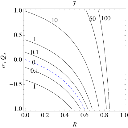
Figure 2: [Left window] : The contour plot of ${\tilde{r}}$ for Case B, $\sigma_{*}=0.05M_{P}$. For the other cases the magnitudes are scaled by $\sigma_{*}^{2}$. Along the blue dashed line ${\tilde{r}}=\delta=0$ . [Right window] : The tensor-to-scalar ratio $r_{T}$ for Case B. The blue shaded region is ruled out using the constraint $r_{T}<0.36$. $\delta=0$ along the blue dashed line.

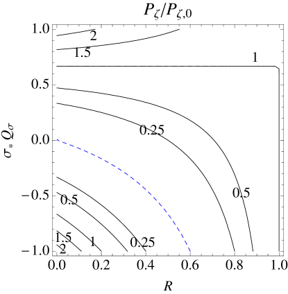
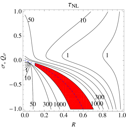
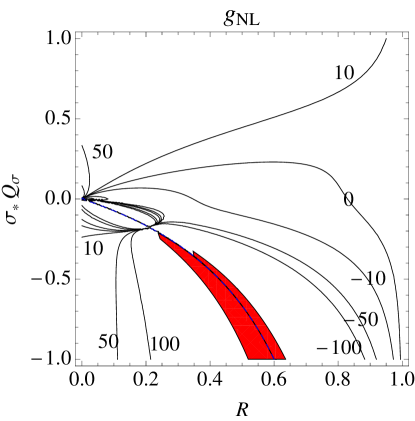
Figure 3: The contour plots on $R-Q_{\sigma}\sigma_{*}$ plane, of the power spectrum ${\cal P}_{\zeta}$ normalized by the value at $R=1$ (upper-left), $f_{\rm NL}$ (upper-right), $\tau_{\rm NL}$ (lower-left) and $g_{\rm NL}$ (lower-right) for Case A, $\sigma_{*}=10^{-3}\,M_{P}$. We put $\eta_{*}=\xi_{*}=0$. The red shaded region corresponds to too large non-Gaussianity to be consistent with the observation, $-10<f_{\rm NL}<73$, $\tau_{\rm NL}<10^{4}$, and $|g_{\rm NL}|<10^{5}$. Along the blue dashed line ${\tilde{r}}=0$ the cancellation happens.

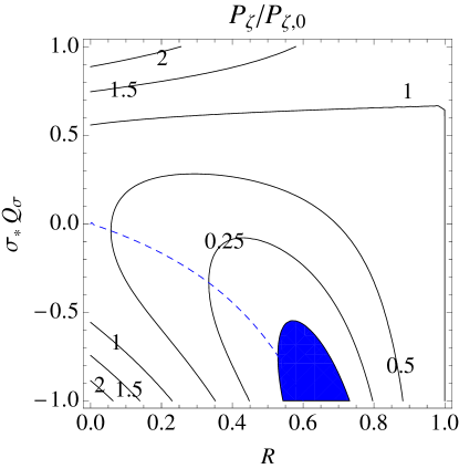
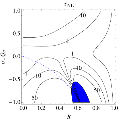
Figure 4: The contour plots on $R-Q_{\sigma}\sigma_{*}$ plane, of the power spectrum ${\cal P}_{\zeta}$ normalized by the value at $R=1$ (upper-left), $f_{\rm NL}$ (upper-right), $\tau_{\rm NL}$ (lower-left) and $g_{\rm NL}$ (lower-right) for Case B, $\sigma_{*}=0.05\,M_{P}$. We put $\eta_{*}=\xi_{*}=0$. The blue shaded region corresponds to too large tensor-to-scalar ratio to be consistent with the observation, $r_{T}<0.36$. Along the blue dashed line $\delta=0$.

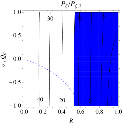
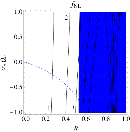
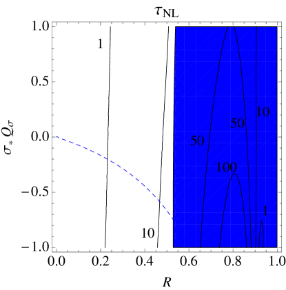
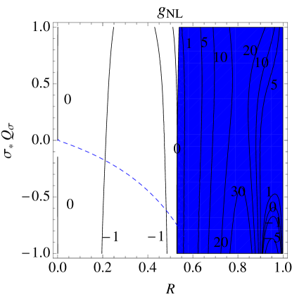
Figure 5: The contour plots on $R-Q_{\sigma}\sigma_{*}$ plane, of the power spectrum ${\cal P}_{\zeta}$ normalized by the value at $R=1$ (upper-left), $f_{\rm NL}$ (upper-right), $\tau_{\rm NL}$ (lower-left) and $g_{\rm NL}$ (lower-right) for Case C, $\sigma_{*}=0.5\,M_{P}$. We put $\eta_{*}=\xi_{*}=0$. The blue shaded region corresponds to too large tensor-to-scalar ratio to be consistent with the observation, $r_{T}<0.36$. Along the blue dashed line $\delta=0$.

In the upper left panel of figures 3 - 5, we show the power spectrum in the plane of $(R,Q_{\sigma}\sigma_{*})$ plane in the upper-left window for each cases with different $\sigma_{*}$ ; $10^{-3}\,M_{P}$ (Case A), $0.05\,M_{P}$ (Case B), $0.5\,M_{P}$ (Case C). We have normalized the amplitude of the power spectrum by the value at the pure curvaton limit of $R=1$, namely ${\cal P}_{\zeta}/{\cal P}_{\zeta,0}$. The slow-roll parameter $\epsilon_{*}$ is calculated from Eq. (28) considering $n_{s}=0.97$ and we used for simplicity $\eta_{*}=\xi_{*}=0$. We assume that the correct observational value can be attained using the residual parameter of $H_{*}$.

The three cases in figures 3 - 5 show the following features:

• Case A : $\sigma_{*}=10^{-3}\,M_{P}$ and ${\tilde{r}}\gg 1$ in most of the region.
  Modulated reheating and curvaton contributions are dominant and inflaton contribution to the curvature perturbation is subdominant,

• Case B : $\sigma_{*}=0.05\,M_{P}$ and ${\tilde{r}}\sim 1$ as shown in figure 2.
  All three contributions are effective,

• Case C : $\sigma_{*}=0.5\,M_{P}$ and ${\tilde{r}}\ll 1$ in most of the region.
  Inflaton contribution is dominant and it scales as $(1-R)^{2}$. $R<0.45$ is allowed from the constraint on the tensor-to-scalar ratio.

In the Case A (upper-left window in figure 3), $\delta\sigma$ contribution is dominant in the overall region and the inflaton contribution is subdominant. In the cancellation region, the relative contribution from $\delta\sigma$ decreases. Of course, by increasing $H_{*}$, the desired amplitude of ${\cal P}_{\zeta}$ can be recovered. The tensor-to-scalar ratio is always much smaller than 0.01 in the shown parameter range.

In the Case B (upper-left window in figure 4), the inflaton contribution is effective for cancellation region and modulation and/or curvaton effects are effective in the rest. The cancellation between the modulated reheating and the curvaton appears around $R\sim 0.7$ for negative $Q_{\sigma}\sigma_{*}$. The tensor-to-scalar ratio is comparable to the observation constraint and a region around $(R,Q_{\sigma}\sigma_{*})\sim(0.6,-1)$ is ruled out as shown in the right window of figure 2.

In the Case C (upper-left window in figure 5), the density perturbation dominantly comes from the inflaton field but the magnitude changes due to the effect of curvaton. For large $R$ the magnitude decreases. A portion of parameter space is excluded because of too large tensor-to-scalar ratio.

III.4 Non-Gaussianity

When the curvaton field dominates the energy density when it decay, i.e. $R\sim 1$, the curvature perturbation is dominated by the pure curvaton and the non-Gaussianity is suppressed. However in the other case $0\lesssim R\ll 1$, there is a possibility to get large non-Gaussianity.

The bispectrum $B_{\zeta}$ is given by

$$\begin{split}\langle\zeta_{\vec{k}_{1}}\zeta_{\vec{k}_{2}}\zeta_{\vec{k}_{3}}\rangle=(2\pi)^{3}B_{\zeta}(k_{1},k_{2},k_{3})\delta(\vec{k_{1}}+\vec{k_{2}}+\vec{k_{3}}),\end{split}$$ (30)

and the dimensionless non-linearity parameter for the bispectrum, $f_{\rm NL}$, is defined by

$$\begin{split}B_{\zeta}(k_{1},k_{2},k_{3})=\frac{6}{5}f_{\rm NL}[P_{\zeta}(k_{1})P_{\zeta}(k_{2})+P_{\zeta}(k_{2})P_{\zeta}(k_{3})+P_{\zeta}(k_{3})P_{\zeta}(k_{1})].\end{split}$$ (31)

From the trispectrum $T_{\zeta}$ given by

$$\begin{split}\langle\zeta_{\vec{k}_{1}}\zeta_{\vec{k}_{2}}\zeta_{\vec{k}_{3}}\zeta_{\vec{k}_{4}}\rangle_{c}=(2\pi)^{3}T_{\zeta}(k_{1},k_{2},k_{3},k_{4})\delta(\vec{k_{1}}+\vec{k_{2}}+\vec{k_{3}}+\vec{k_{4}}),\end{split}$$ (32)

the dimensionless non-linearity parameters $\tau_{\rm NL}$ and $g_{\rm NL}$ are defined as astro-ph/0611075

$$\begin{split}T_{\zeta}(k_{1},k_{2},k_{3},k_{4})=&\tau_{\rm NL}[P_{\zeta}(k_{13})P_{\zeta}(k_{3})P_{\zeta}(k_{4})+11\text{ perms}]\\ &+\frac{54}{25}g_{\rm NL}[P_{\zeta}(k_{2})P_{\zeta}(k_{3})P_{\zeta}(k_{4})+3\text{ perms}].\end{split}$$ (33)

The current bounds have been derived by several groups Smidt:2010ra ; Fergusson:2010gn . For instance, Smidt et. al. reported as $-7.4<g_{\rm NL}10^{-5}<8.2$ and $-0.6<\tau_{\rm NL}10^{-4}<3.3$ Smidt:2010ra .

In figure 3, we show the contours of the non-linearity parameters $f_{\rm NL}$ (upper-right window), $\tau_{\rm NL}$ (lower-left window) and $g_{\rm NL}$ (lower-right window) for the Case A. For the contours we have taken account the relations, $Q_{\sigma\sigma}\sigma_{*}^{2}=Q_{\sigma}\sigma_{*}(6Q_{\sigma}\sigma_{*}+1)$ and $Q_{\sigma\sigma\sigma}\sigma_{*}^{3}=12Q_{\sigma}\sigma_{*}Q_{\sigma\sigma}\sigma_{*}^{3}$, which are motivated from the specific example we will show in the next section. We can see clearly the enhancement of non-linearity parameters in the cancellation region of modulated reheating and curvaton. The pure curvaton limit is recovered along the line of $Q_{\sigma}\sigma_{*}=0$.

In figure 4 for the Case B, we can see the enhancement of the non-linearity parameters along the cancellation region. The difference from the Case A is that now the inflaton becomes more important and diminishes the non-Gaussinaity.

In both cases of A and B, the large non-Gaussianity is dominantly due to $\delta\sigma$, while the power spectrum comes from both depending on ${\tilde{r}}$, as explained in the Appendix. The non-linearity parameters can be enhanced around the cancellation region ($\delta\ll 1$ and $\delta\ll{\tilde{r}}$). In this region, a large $f_{\rm NL}$ comes dominantly from $\zeta_{2,\sigma\sigma}$ as defined in Eq. (LABEL:zeta123A) of the Appendix and estimated to be

$$\begin{split}f_{\rm NL}\simeq\frac{5}{6}\frac{{\tilde{r}}^{2}}{(1+{\tilde{r}})^{2}}\frac{1}{\delta^{2}}\frac{9(1-R)Q_{\sigma\sigma}\sigma_{*}^{2}-6R+R(1-R)(3+R)(Q_{\sigma}\sigma_{*}-2)^{2}}{4R^{2}}.\end{split}$$ (34)

Therefore small $\delta$ (large cancellation due to fine-tuning) can induce larger $f_{\rm NL}$. However note that ${\tilde{r}}$ is proportional to $\delta^{2}$ (so ${\tilde{r}}^{2}\propto\delta^{4}$), thus too small $\delta$ makes ${\tilde{r}}$ becomes smaller than $\delta$ itself and reduces $f_{\rm NL}$. One can see this behavior clearly in the upper right figure of figure 4: $f_{\rm NL}$ decreases when approaching the cancellation line (blue dashed line).

In the same region $\tau_{\rm NL}$ is also dominated by $\zeta_{2,\sigma\sigma}$ term and approximately the squared of $f_{\rm NL}$,

$$\begin{split}\tau_{\rm NL}\simeq{\left(\frac{1+{\tilde{r}}}{{\tilde{r}}}\right)}\left(\frac{6}{5}f_{\rm NL}\right)^{2}.\end{split}$$ (35)

Large $g_{\rm NL}$ is possible in the same cancellation region dominated by $\zeta_{3,\sigma\sigma\sigma}$ term and given by

$$\begin{split}g_{\rm NL}\simeq\frac{25}{54}&\frac{{\tilde{r}}^{3}}{(1+{\tilde{r}})^{3}}\frac{1}{\delta^{3}}\frac{1}{8R^{3}}\\ \times[&9(1-R)Q_{\sigma\sigma\sigma}\sigma_{*}^{3}+9R(1-R)(3+R)(3Q_{\sigma}\sigma_{*}-2)(3Q_{\sigma\sigma}\sigma_{*}^{2}+2)\\ &+36R+R(1-R)(3+R)(-3+4R+3R^{2})(3Q_{\sigma}\sigma_{*}-2)^{3}].\end{split}$$ (36)

As you can see here, $g_{\rm NL}$ has different sign in the opposite side of the cancellation line due to the odd exponent ’3’ of $\delta$.

Here one can see that there are two points in both sides of $3Q_{\sigma}\sigma_{*}\simeq-2R/(1-R)$ those give the same values of ${\cal P}_{\zeta}$ and $f_{\rm NL}$. This means that the measurements of only ${\cal P}_{\zeta}$ and $f_{\rm NL}$ can not determine $R$ and $Q_{\sigma}\sigma_{*}$ uniquely. However, this degeneracy can be resolved by measuring $g_{\rm NL}$ because one predicts $g_{\rm NL}$ to be positive and the other does it to be negative.

In figure 5 for the Case C, the region of large non-linearity parameters are in the region of $R>0.5$ but which is excluded out by large $r_{T}$.

IV A simple model

As we have seen in the previous sections, if a light scalar curvaton field $\sigma$ has an interaction with inflaton field $\phi$, the fluctuation of curvaton field $\delta\sigma$ can modulate reheating through the decay of inflaton and can affect the curvature perturbation besides the usual curvaton mechanism. The resultant power spectrum and the non-linearity parameters can be considerably affected. In this section, we examine these effects in a simple model.

The inflaton $\phi$ and the curvaton $\sigma$ can have the following interactions in the scalar potential

$$V[\phi,\sigma]=\frac{1}{2}m_{\phi}^{2}\phi^{2}+\frac{1}{2}m_{\sigma}^{2}\sigma^{2}+\frac{1}{2}\lambda_{\phi\sigma}\phi^{2}\sigma^{2},$$ (37)

as well as an interaction with another scalar field as given in Eq. (1). It is also possible that the inflaton has interaction with other fields independent from the curvaton. We consider that the inflation is dominantly driven by a single inflaton field with its quadratic mass term potential by assuming $m_{\phi}\gg m_{\sigma}$ and

$$m_{\phi}^{2}\gg\lambda_{\phi\sigma}\sigma_{*}^{2}.$$ (38)

We consider cases of vanishing $\lambda_{\phi\sigma}$ in subsection IV.1 and IV.2, and mention the effect of nonvanishing $\lambda_{\phi\sigma}$ in subsection IV.3. Its interactions with other fields are important during reheating or later. Therefore during inflation, field equations are reduced to

$$H^{2}=\frac{1}{6M_{P}^{2}}m_{\phi}^{2}\phi^{2},$$ (39)

$$3H\dot{\phi}+m_{\phi}^{2}\phi=0,$$ (40)

under the slow-roll condition

$$\begin{split}\epsilon\equiv\frac{M_{P}^{2}}{2}{\left(\frac{V_{\phi}}{V}\right)}^{2}\simeq\frac{2M_{P}^{2}}{\phi^{2}}\ll 1,\qquad\eta\equiv\frac{M_{P}^{2}V_{\phi\phi}}{V}\ll 1,\end{split}$$ (41)

and the inflaton-domination condition

$$\frac{1}{2}m_{\phi}^{2}\phi^{2}\gg\frac{1}{2}m_{\sigma}^{2}\sigma^{2}.$$ (42)

By solving field equations, we obtain

$$\phi_{*}^{2}=(4N_{\rm inf}+2)M_{P}^{2},$$ (43)

where $N_{\rm inf}$ is the number of e-fold at horizon exit from the end of inflation. The power spectrum is

$${\cal P}_{\zeta}\simeq\frac{(1-R)^{2}}{6(2\pi)^{2}}\frac{m_{\phi}^{2}}{M_{P}^{2}}(2N_{\rm inf}+1)^{2}+\left\{(1-R)Q_{\sigma}\sigma_{*}+\frac{2R}{3}\right\}^{2}\frac{m_{\phi}^{2}}{3(2\pi\sigma_{*})^{2}}(2N_{\rm inf}+1).$$ (44)

The inflaton mass $m_{\phi}$ controls the amplitude of the density perturbation. For the observed ${\cal P}_{\zeta}$ we can estimate $m_{\phi}$.

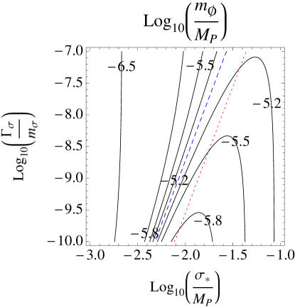
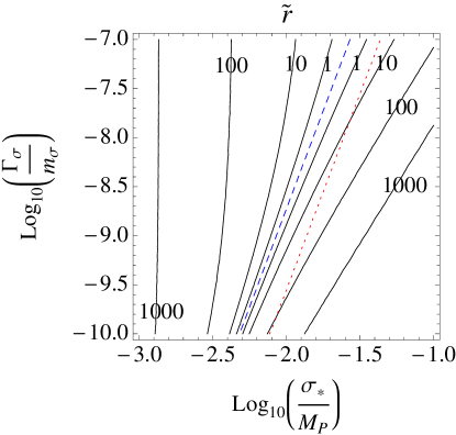
Figure 6: [Left window] : The contour plot of $m_{\phi}$ of the Model I in the unit of $\log_{10}\left(\frac{m_{\phi}}{M_{P}}\right)$ where ${\cal P}_{\zeta}$ has been fixed by the observed value ${\cal P}_{\zeta}=2.44\times 10^{-9}$. In the left side of the red line radiation is dominated at the time of curvaton decay and in the right side curvaton dominates. The cancellation between curvaton and modulated reheating occurs along the blue line where ${\tilde{r}}=0$. [Right window] : The contour plot of ${\tilde{r}}$. The red and blue lines are the same as in the left window.

It is natural to assume that inflaton decays at its oscillating stage after a while, so that $\Gamma_{\phi}(\sigma)/m_{\phi}$ is very small. In this case $Q$ is well approximated by Suyama:2007bg

$$\begin{split}Q\simeq-\frac{1}{6}\log{\left(\frac{\Gamma_{\phi}(\sigma)}{H_{c}}\right)}.\end{split}$$ (45)

The derivatives are expressed as

$$Q_{\sigma} = -\frac{1}{6}\frac{\partial_{\sigma}\Gamma_{\phi}}{\Gamma_{\phi}},$$ (46)

$$Q_{\sigma\sigma} = -\frac{1}{6}\left(\frac{\partial_{\sigma}^{2}\Gamma_{\phi}}{\Gamma_{\phi}}-\frac{(\partial_{\sigma}\Gamma_{\phi})^{2}}{\Gamma^{2}_{\phi}}\right),$$ (47)

$$Q_{\sigma\sigma\sigma} = -\frac{1}{6}\left(\frac{\partial_{\sigma}^{3}\Gamma_{\phi}}{\Gamma_{\phi}}-3\frac{\partial_{\sigma}\Gamma_{\phi}\partial^{2}_{\sigma}\Gamma_{\phi}}{\Gamma^{2}_{\phi}}+2\frac{(\partial_{\sigma}\Gamma_{\phi})^{3}}{\Gamma^{3}_{\phi}}\right).$$ (48)

IV.1 Model I : Inflaton decays through only the coupling in Eq. (1)

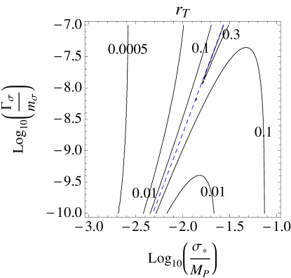
Figure 7: The contour plot of $r_{T}$ for the Model I. The blue line shows ${\tilde{r}}=0$.

First, let us consider the case that the inflaton $\phi$ decays through only the coupling in Eq. (1). For this case, we obtain

$$(Q_{\sigma}\sigma_{*},Q_{\sigma\sigma}\sigma_{*}^{2},Q_{\sigma\sigma\sigma}\sigma_{*}^{3})=\left(\begin{array}[]{ccc}-\frac{1}{3},&\frac{1}{3},&-\frac{2}{3}\end{array}\right).$$ (49)

The parameter defined in Eq. (15) at the time of curvaton decay is can be obtained using Eqs. (5) - (6) by

$$R=\frac{\sigma_{*}^{2}/M_{P}^{2}}{8(a_{m_{\sigma}}/a_{\Gamma_{\sigma}})+\sigma_{*}^{2}/M_{P}^{2}},$$ (50)

with

$$\frac{a_{m_{\sigma}}}{a_{\Gamma_{\sigma}}}=\left\{\begin{array}[]{l}\left(\frac{\Gamma_{\sigma}}{m_{\sigma}}\right)^{1/2}\qquad\qquad\qquad{\rm radiation-dominated}\\ \left(\frac{\sigma_{*}^{2}}{6M_{P}^{2}}\right)^{-1/3}\left(\frac{\Gamma_{\sigma}}{m_{\sigma}}\right)^{2/3}\quad\quad\sigma{\rm-dominated}\end{array}\right..$$ (51)

Here $\Gamma_{\sigma}$ is the decay rate of the curvaton field and $a_{m_{\sigma}}/a_{\Gamma_{\sigma}}$ is expressed in different ways depending on whether it is radiation-dominated or curvaton-dominated when the curvaton decays at $H=\Gamma_{\sigma}$.

In this case, there are only three parameters $m_{\phi},\sigma_{*}$ and $\Gamma_{\sigma}/m_{\sigma}$, since $Q_{\sigma}\sigma_{*}$ and so on are completely fixed. As mentioned above, from the normalization of the power spectrum, $m_{\phi}$ can be expressed by the other two parameters as shown in the left window of figure 6. The largest value to $m_{\phi}$ in figure 6 seems to be $10^{-5.2}M_{P}$ which is the same as the results in the quadratic chaotic inflation. This is because the region corresponds to the cancellation, $3Q_{\sigma}\sigma_{*}\simeq-2R/(1-R)$ line (blue line and $R=1/3$ in this case), where ${\tilde{r}}\simeq 0$ and the contribution from $\sigma$ field cancels, and the dominant contribution comes from $\phi$ field. On the other hand, $\sigma$ contribution is not negligible in other regions and hence a smaller $m_{\phi}$ is needed to produce the observable ${\cal P}_{\zeta}$. In the right window of figure 6, we showed a contour plot of ${\tilde{r}}$. We note that the condition for a negligible $\lambda_{\phi\sigma}$, Eq. (38), can be rewritten as

$$\lambda_{\phi\sigma}\ll 10^{-6}\left(\frac{m_{\phi}}{10^{-5}M_{P}}\right)^{2}\left(\frac{10^{-2}M_{P}}{\sigma_{*}}\right)^{2}.$$ (52)

In figure 7, we showed the contour plot of $r_{T}$. The present bound on the $r_{T}$ does not constrain this model, however future bound can rule out the parameter range around the cancellation region along the blue line.

In figure 8, the non-linearity parameters $f_{\rm NL}$ (left) and $g_{\rm NL}$ (right) are shown.

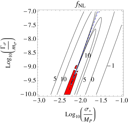
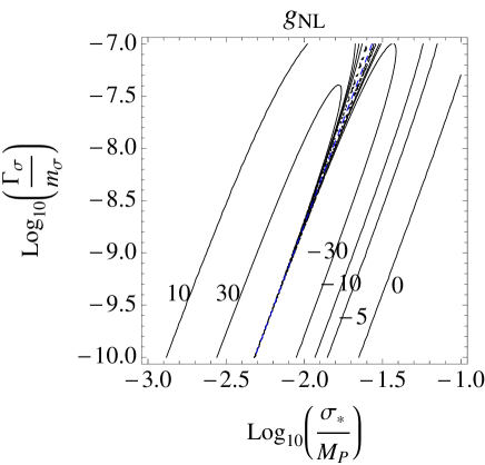
Figure 8: [Left window] : The contour plot of $f_{\rm NL}$ in $(\sigma_{*}/M_{P},\Gamma_{\sigma}/m_{\sigma})$ plain for the Model I. The red shaded region corresponds to too large $f_{\rm NL}$ to be consistent with the observation. [Right window] : The contour of $g_{\rm NL}$ for the Model I.

IV.2 Model II : Inflaton decays through the coupling in Eq. (1) and others

Next, let us consider the case that the inflaton $\phi$ has a nonvanishing $\sigma$ independent decay modes and the total decay width is given by Eq. (4). For this case, we obtain

$$(Q_{\sigma}\sigma_{*},Q_{\sigma\sigma}\sigma_{*}^{2},Q_{\sigma\sigma\sigma}\sigma_{*}^{3})=\left(\begin{array}[]{ccc}-\frac{1}{3}Br,&\frac{1}{3}Br(2Br-1),&-\frac{2}{3}Br^{2}(4Br-3)\end{array}\right),$$ (53)

with $Br\equiv\Gamma_{\phi}^{(CD)}/\Gamma_{\phi}$. Obviously, the $Br\rightarrow 1$ limit reduces to the Model I in the previous subsection. In this case, we have four parameters $m_{\phi},\sigma_{*},\Gamma_{\sigma}/m_{\sigma}$ and $Br$. Again, $m_{\phi}$ can be used for the normalization of the power spectrum. In figure 9, we show the contour plot of $f_{\rm NL}$ for $Br=0.3$ (left) and $0.1$ (right). As we have seen, the cancellation happens at $3Q_{\sigma}\sigma_{*}\simeq-2R/(1-R)$ or $R\simeq Br/(2+Br)$.

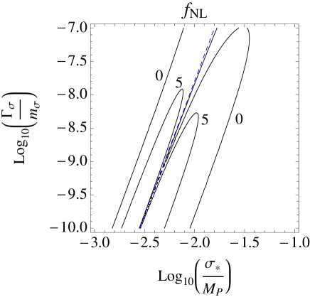
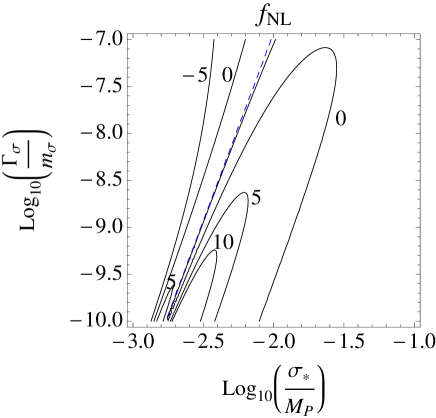
Figure 9: [Left window] : The contour plot of $f_{\rm NL}$ with $Br=0.3$ on $(\sigma_{*}/M_{P},\Gamma_{\sigma}/m_{\sigma})$ plane for the Model II. The red shaded region corresponds to too large $f_{\rm NL}$ to be consistent with the observation. [Right window] : The same as left window but with $Br=0.1$.

IV.3 Model III : The effective inflaton mass with the coupling in Eq. (3)

Finally, let us consider the case of nonvanishing $\lambda_{\phi\sigma}$. Then, through just only the coupling (3), in other words even without direct coupling (1), the inflaton decay width $\Gamma\sim M_{\phi}^{3}/M_{P}^{2}$ with the effective inflaton mass $M_{\phi}^{2}=m_{\phi}^{2}+\lambda_{\phi\sigma}\sigma_{*}^{2}$ which is $\sigma$ dependent.

For this case, we obtain

$$(Q_{\sigma}\sigma_{*},Q_{\sigma\sigma}\sigma_{*}^{2},Q_{\sigma\sigma\sigma}\sigma_{*}^{3})=\left(\begin{array}[]{ccc}-\frac{1}{2}Fr,&\frac{1}{2}Fr(2Fr-1),&Fr^{2}(3-4Fr)\end{array}\right),$$ (54)

with $Fr\equiv\lambda_{\phi\sigma}\sigma_{*}^{2}/M_{\phi}^{2}$. The qualitative behavior of this model is the same as that of the Model II up to numerical factors, by replacing $Br$ with $Fr$.

V Conclusion

We have studied the case where a light scalar field $\sigma$ induces the modulated reheating by the inflaton decay and also acts as the curvaton by its late time decay in the presence of the curvature perturbation generated from the inflaton field itself. In fact, the coupling in Eq. (1) is possible from the gauge invariance of the SM , provided both $\phi$ and $\sigma$ are gauge singlet as is often assumed to preserve the flatness of the potential.

When $\sigma$ field contributes to both inducing the modulated reheating by the inflaton decay and generating the density perturbation as the curvaton, there could be a cancellation between two contributions along the line $3Q_{\sigma}\sigma_{*}\simeq-2R/(1-R)$. Around this cancellation region, $\delta\sigma$ contribution to the power spectrum of the density perturbation is subdominant and the inflaton contribution becomes dominant. Near such a parameter region, mostly the middle range of $R$ and a negative $Q_{\sigma}\sigma_{*}$, non-linearity parameters tend to be large because of the cancellation between the modulated reheating and the curvaton originated from the same field $\sigma$. In this sense, this cancellation is a kind of mechanisms to generate a large non-Gaussianity

As specific models, we have also studied a quadratic inflation and curvaton model and demonstrated how the parameter space of a given inflaton and curvaton model would be constrained by taking the interaction between them into account. The measurement of non-linearity and tensor-to-scalar ratio may probe the strength of (non-)interaction between the inflaton and the curvaton.

Appendix A Large non-Gaussianity

The curvature perturbation $\zeta$ can be decomposed of the contributions from each field perturbations order by order as

$$\zeta=\zeta_{1}+\frac{1}{2}\zeta_{2}+\frac{1}{6}\zeta_{3}+\ldots,$$ (55)

with

$$\begin{split}\zeta_{1}=&\zeta_{1,\phi}\delta\phi+\zeta_{1,\sigma}\delta\sigma,\\ \zeta_{2}=&\zeta_{2,\phi\phi}(\delta\phi)^{2}+2\zeta_{2,\phi\sigma}(\delta\phi)(\delta\sigma)+\zeta_{2,\sigma\sigma}(\delta\sigma)^{2},\\ \zeta_{3}=&\zeta_{3,\phi\phi\phi}(\delta\phi)^{2}+3\zeta_{3,\phi\phi\sigma}(\delta\phi)^{2}(\delta\sigma)+3\zeta_{3,\phi\sigma\sigma}(\delta\phi)(\delta\sigma)^{2}+\zeta_{3,\sigma}(\delta\sigma)^{3}.\\ \ldots&\end{split}$$ (56)

Here we considered two-field case for simplicity and we suppressed $*$ which denotes the value at horizon exit, i.e. $\delta\phi=\delta\phi_{*}$ and $\delta\sigma=\delta\sigma_{*}$. For the model of modulated reheating by curvaton, we can read each component from Eq. (19).

The power spectrum is given from Eq. (20) by

$$\begin{split}{\cal P}_{\zeta}=(\zeta_{1,\phi}^{2}+\zeta_{1,\sigma}^{2}){\left(\frac{H_{*}}{2\pi}\right)}^{2}=\zeta_{1,\phi}^{2}(1+{\tilde{r}}){\left(\frac{H_{*}}{2\pi}\right)}^{2},\end{split}$$ (57)

where we used Eq. (22) and ${\tilde{r}}\equiv\zeta_{1,\sigma}^{2}/\zeta_{1,\phi}^{2}$. From the definitions in Eq. (31) and Eq. (33), the non-Gaussianity parameters are given by

$$\begin{split}f_{\rm NL}=&\frac{5}{6}\frac{\zeta_{1,\phi}^{2}\zeta_{2,\phi\phi}+2\zeta_{1,\phi}\zeta_{1,\sigma}\zeta_{2,\phi\sigma}+\zeta_{1,\sigma}^{2}\zeta_{2,\sigma\sigma}}{(\zeta_{1,\phi}^{2}+\zeta_{1,\sigma}^{2})^{2}},\\ \tau_{\rm NL}=&\frac{\sum_{a,b,c}\zeta_{1,b}\zeta_{1,c}\zeta_{2,ab}\zeta_{2,ac}}{(\zeta_{1,\phi}^{2}+\zeta_{1,\sigma}^{2})^{3}},\\ g_{\rm NL}=&\frac{25}{54}\frac{\sum_{a,b,c}\zeta_{1,a}\zeta_{1,b}\zeta_{1,c}\zeta_{3,abc}}{(\zeta_{1,\phi}^{2}+\zeta_{1,\sigma}^{2})^{3}}.\end{split}$$ (58)

Here $a,b,c$ denotes $\phi$ and $\sigma$.

First we will investigate the condition for large $f_{\rm NL}$ in the curvaton-modulated scenario. Using Eq. (19), the denominator of $f_{\rm NL}$ in Eq. (58) becomes

$$\begin{split}(\zeta_{1,\phi}^{2}+\zeta_{1,\sigma}^{2})^{2}=\left[\frac{1}{2M_{P}^{2}\epsilon_{*}}(1-R)^{2}(1+{\tilde{r}})\right]^{2}\sim\frac{(1+{\tilde{r}})^{2}}{M_{P}^{4}\epsilon_{*}^{2}},\end{split}$$ (59)

where in the last equation we dropped $\mathcal{O}(1)$ coefficient, $R$ and $Q_{\sigma}\sigma$. In the same way, the numerators are

$$\begin{split}\zeta_{1,\phi}^{2}\zeta_{2,\phi\phi}=&\frac{1}{4M_{P}^{4}\epsilon_{*}^{2}}(1-R)^{3}[R(R+3)+2\epsilon_{*}-\eta_{*}]\sim\frac{1}{M_{P}^{4}\epsilon_{*}^{2}},\\ 2\zeta_{1,\phi}\zeta_{1,\sigma}\zeta_{2,\phi\sigma}=&\frac{1}{9M_{P}^{2}\epsilon_{*}\sigma^{2}}R(1-R)^{2}(3+R)[3Q_{\sigma}\sigma(1-R)+2R][3Q\sigma-2]\sim\frac{1}{M_{P}^{4}\epsilon_{*}^{2}}\frac{{\tilde{r}}}{\delta},\\ \zeta_{1,\sigma}^{2}\zeta_{2,\sigma\sigma}=&\frac{1}{81\sigma^{4}}[3Q_{\sigma}\sigma(1-R)+2R]^{2}[9Q_{\sigma\sigma}\sigma^{2}(1-R)-6R+R(1-R)(3+R)(3Q_{\sigma}\sigma-2)^{2}]\\ \sim&\frac{1}{M_{P}^{4}\epsilon_{*}^{2}}\frac{{\tilde{r}}^{2}}{\delta^{2}}.\end{split}$$ (60)

Therefore we find that large $f_{\rm NL}$ can arise from the last term $\zeta_{1,\sigma}^{2}\zeta_{2,\sigma\sigma}$ to give

$$\begin{split}f_{\rm NL}\sim\frac{{\tilde{r}}^{2}}{(1+{\tilde{r}})^{2}}\frac{1}{\delta^{2}}.\end{split}$$ (61)

It is easy to see that

$$\begin{split}f_{\rm NL}\sim\frac{1}{\delta^{2}}\qquad\text{for}\qquad{\tilde{r}}\gtrsim 1,\qquad\text{and}\qquad\delta\ll 1.\end{split}$$ (62)

and

$$\begin{split}f_{\rm NL}\sim\frac{{\tilde{r}}^{2}}{\delta^{2}}\qquad\text{for}\qquad{\tilde{r}}\lesssim 1,\qquad\text{and}\qquad\delta\ll{\tilde{r}}.\end{split}$$ (63)

However ${\tilde{r}}$ and $\delta$ are not independent variables and ${\tilde{r}}$ is proportional to $\delta^{2}$ in our case as in Eq. (27). Therefore for a given parameters, $f_{\rm NL}$ vanishes in the limit of $\delta\rightarrow 0$ when ${\tilde{r}}$ becomes vanishing too. The large $f_{\rm NL}$ can arise whenl $\delta$ is smaller than 1 and smaller than ${\tilde{r}}$.

Similarly, large $\tau_{\rm NL}$ and $g_{\rm NL}$ are obtained in the same region as that of $f_{\rm NL}$ when $\zeta_{2,\sigma\sigma}$ and $\zeta_{3,\sigma\sigma\sigma}$ term dominates and are estimated to be

$$\begin{split}\tau_{\rm NL}\sim\frac{{\tilde{r}}^{3}}{(1+{\tilde{r}})^{3}}\frac{1}{\delta^{4}},\qquad\text{and}\qquad g_{\rm NL}\sim\frac{{\tilde{r}}^{3}}{(1+{\tilde{r}})^{3}}\frac{1}{\delta^{3}}.\end{split}$$ (64)

We find that $g_{\rm NL}$ is smaller than $\tau_{\rm NL}$ in the large non-Gaussianity region.

References

-
(1)
A. A. Starobinsky,
JETP Lett. 30 682 (1979)
[Pisma Zh. Eksp. Teor. Fiz. 30 719 (1979)];
K. Sato, Mon. Not. Roy. Astron. Soc. 195, 467 (1981);
A. H. Guth, Phys. Rev. D 23, 347 (1981);
A. D. Linde, Phys. Lett. B 108 389 (1982);
A. Albrecht and P. J. Steinhardt, Phys. Rev. Lett. 48 1220 (1982). -
(2)
S. W. Hawking,
Phys. Lett. B 115, 295 (1982);
A. A. Starobinsky, Phys. Lett. B 117, 175 (1982);
A. H. Guth and S. Y. Pi, Phys. Rev. Lett. 49, 1110 (1982). - (3) J. M. Maldacena, JHEP 0305, 013 (2003).
- (4) E. Komatsu et al., Astrophys. J. Suppl. 192, 18 (2011).
- (5) http://www.rssd.esa.int/index.php?project=PLANCK
- (6) K. Y. Choi, L. M. H. Hall and C. van de Bruck, JCAP 0702 029 (2007).
- (7) C. T. Byrnes, K. Y. Choi and L. M. H. Hall, JCAP 0810 008 (2008).
- (8) C. T. Byrnes, K. Y. Choi and L. M. H. Hall, JCAP 0902 017 (2009).
- (9) B. Kyae, Eur. Phys. J. C 72 1857 (2012).
- (10) J. Elliston, D. J. Mulryne, D. Seery and R. Tavakol, JCAP 1111 005 (2011); Int. J. Mod. Phys. A 26 3821 (2011).
- (11) K. -Y. Choi and B. Kyae, Phys. Lett. B 706 243 (2012).
- (12) D. H. Lyth, JCAP 0511 006 (2005).
- (13) L. Alabidi and D. Lyth, JCAP 0608 006 (2006).
- (14) M. Sasaki, Prog. Theor. Phys. 120 159 (2008).
- (15) A. Naruko and M. Sasaki, Prog. Theor. Phys. 121, 193 (2009).
- (16) K. -Y. Choi, S. A. Kim and B. Kyae, arXiv:1202.0089 [astro-ph.CO].
-
(17)
K. Enqvist, A. Jokinen, A. Mazumdar, T. Multamaki and A. Vaihkonen,
Phys. Rev. Lett. 94 161301 (2005); JCAP 0503 010 (2005);
A. Jokinen and A. Mazumdar, JCAP 0604 003 (2006). -
(18)
for a recent review on local type non-Gaussianity, see e.g.,
C. T. Byrnes and K. Y. Choi,
Adv. Astron. 2010, 724525 (2010) ;
D. Wands, Class. Quant. Grav. 27, 124002 (2010). - (19) S. Mollerach, Phys. Rev. D 42 313 (1990).
- (20) A. D. Linde and V. F. Mukhanov, Phys. Rev. D 56 535 (1997).
- (21) D. H. Lyth and D. Wands, Phys. Lett. B 524, 5 (2002).
- (22) T. Moroi and T. Takahashi, Phys. Lett. B 522, 215 (2001) [Erratum-ibid. B 539, 303 (2002)].
- (23) K. Enqvist and M. S. Sloth, Nucl. Phys. B 626, 395 (2002).
- (24) D. H. Lyth, C. Ungarelli and D. Wands, Phys. Rev. D 67, 023503 (2003).
-
(25)
D. Langlois and F. Vernizzi,
Phys. Rev. D 70, 063522 (2004);
G. Lazarides, R. R. de Austri and R. Trotta, Phys. Rev. D 70, 123527 (2004);
F. Ferrer, S. Rasanen and J. Valiviita, JCAP 0410, 010 (2004);
T. Moroi, T. Takahashi and Y. Toyoda, Phys. Rev. D 72 023502 (2005);
T. Moroi and T. Takahashi, Phys. Rev. D 72 023505 (2005);
K. Ichikawa, T. Suyama, T. Takahashi and M. Yamaguchi, Phys. Rev. D 78, 023513 (2008). - (26) G. Dvali, A. Gruzinov and M. Zaldarriaga, Phys. Rev. D 69 023505 (2004).
- (27) L. Kofman, arXiv:astro-ph/0303614.
- (28) M. Zaldarriaga, Phys. Rev. D 69, 043508 (2004).
- (29) C. W. Bauer, M. L. Graesser and M. P. Salem, Phys. Rev. D 72 023512 (2005).
- (30) T. Suyama and M. Yamaguchi, Phys. Rev. D 77, 023505 (2008).
- (31) K. Ichikawa, T. Suyama, T. Takahashi, M. Yamaguchi, Phys. Rev. D78 063545 (2008).
- (32) B. A. Bassett, S. Tsujikawa and D. Wands, Rev. Mod. Phys. 78, 537 (2006).
- (33) T. Suyama, T. Takahashi, M. Yamaguchi and S. Yokoyama, JCAP 1012 (2010) 030.
- (34) For a review, see.e.g., K. Enqvist, Prog. Theor. Phys. Suppl. 190, 62 (2011).
-
(35)
K. Dimopoulos, G. Lazarides, D. Lyth and R. Ruiz de Austri,
Phys. Rev. D 68 123515 (2003);
K. Enqvist and S. Nurmi, JCAP 0510 013 (2005);
K. Enqvist and T. Takahashi, JCAP 0809, 012 (2008);
Q. G. Huang and Y. Wang, JCAP 0809 025 (2008);
Q. G. Huang, JCAP 0811, 005 (2008);
M. Kawasaki, K. Nakayama and F. Takahashi, JCAP 0901, 026 (2009);
P. Chingangbam and Q. G. Huang, JCAP 0904, 031 (2009);
K. Enqvist, S. Nurmi, G. Rigopoulos, O. Taanila and T. Takahashi, JCAP 0911, 003 (2009);
K. Enqvist and T. Takahashi, JCAP 0912, 001 (2009);
K. Enqvist, S. Nurmi, O. Taanila and T. Takahashi, JCAP 1004, 009 (2010);
Q. G. Huang, JCAP 1011, 026 (2010) [Erratum-ibid. 1102, E01 (2011)];
C. T. Byrnes, K. Enqvist and T. Takahashi, JCAP 1009, 026 (2010);
K. -Y. Choi and O. Seto, Phys. Rev. D 82 103519 (2010);
J. Fonseca and D. Wands, Phys. Rev. D 83, 064025 (2011);
C. T. Byrnes, K. Enqvist, S. Nurmi and T. Takahashi, JCAP 1111, 011 (2011);
M. Kawasaki, T. Kobayashi and F. Takahashi, Phys. Rev. D 84, 123506 (2011) [Phys. Rev. D 85, 029905 (2012)]. - (36) N. Bartolo, S. Matarrese and A. Riotto, Phys. Rev. D 69 043503 (2004).
- (37) D. H. Lyth and Y. Rodriguez, Phys. Rev. Lett. 95 121302 (2005).
- (38) M. Sasaki, J. Valiviita and D. Wands, Phys. Rev. D 74 103003 (2006).
-
(39)
C. T. Byrnes, M. Sasaki and D. Wands,
Phys. Rev. D 74 123519 (2006);
D. Seery and J. E. Lidsey, JCAP 0701, 008 (2007). - (40) J. Smidt, A. Amblard, C. T. Byrnes, A. Cooray, A. Heavens and D. Munshi, Phys. Rev. D 81, 123007 (2010).
- (41) J. R. Fergusson, D. M. Regan and E. P. S. Shellard, arXiv:1012.6039 [astro-ph.CO].