A search for 21 cm H I absorption in AT20G compact radio galaxies

Abstract

We present results from a search for 21 cm associated H i absorption in a sample of 29 radio sources selected from the Australia Telescope 20 GHz survey. Observations were conducted using the Australia Telescope Compact Array Broadband Backend, with which we can simultaneously look for 21 cm absorption in a redshift range of $0.04\lesssim z\lesssim 0.08$, with a velocity resolution of 7 km s^-1. In preparation for future large-scale H i absorption surveys we test a spectral-line finding method based on Bayesian inference. We use this to assign significance to our detections and to determine the best-fitting number of spectral-line components. We find that the automated spectral-line search is limited by residuals in the continuum, both from the band-pass calibration and spectral-ripple subtraction, at spectral-line widths of $\Delta{v}_{\mathrm{FWHM}}\gtrsim 10^{3}$ km s^-1. Using this technique we detect two new absorbers and a third, previously known, yielding a 10 per cent detection rate. Of the detections, the spectral-line profiles are consistent with the theory that we are seeing different orientations of the absorbing gas, in both the host galaxy and circumnuclear disc, with respect to our line-of-sight to the source. In order to spatially resolve the spectral-line components in the two new detections, and so verify this conclusion, we require further high-resolution 21 cm observations ($\sim 0.01$ arcsec) using very long baseline interferometry.

1 Introduction

Observations of the 21 cm H i line of neutral atomic hydrogen in absorption against bright radio continuum sources can provide a unique probe of the distribution and kinematics of gas in the innermost regions of radio galaxies. For a fixed background continuum source brightness the detection limit for H i and molecular absorption lines is independent of the redshift of the absorber. Therefore measurements of associated H i absorption in active galaxies are sensitive to relatively small amounts of neutral gas, provided the central radio continuum source is sufficiently strong and compact. H i absorption-line measurements can detect both circumnuclear gas discs and large scale gas, including inflows and outflows related to to Active Galactic Nuclei (AGN) fuelling and feedback (e.g. Morganti et al. 2001; Holt, Tadhunter, & Morganti 2008; Morganti et al. 2011). Recent studies by Morganti and colleagues have found broad, shallow absorption-line components arising from the large-scale gas outflows in radio galaxies (Morganti, Tadhunter, & Oosterloo 2005; Holt et al. 2008), which provide some of the most direct evidence for AGN-driven feedback in massive galaxies (Croton et al., 2006).

Previous work may suggest that the detection rate of associated H i absorption is highest in the most compact radio galaxies, Morganti et al. (2001) searched for H i absorption in 23 nearby ($z<0.22$) radio galaxies from the southern 2 Jy sample (Morganti et al., 1999), from which they obtained five detections (an overall detection rate of 22 per cent). They found that the H i detection rate in compact radio galaxies was much higher than in classical FR-i and broad emission-line FR-ii systems. Furthermore Vermeulen et al. (2003) detected H i absorption in 19 (33 per cent) of a sample of 57 compact radio galaxies at $z<0.85$. Pihlström, Conway, & Vermeulen (2003) show that the integrated optical depth for 21 cm H i absorption increases with decreasing source size, suggesting that the probability of detection might be highest for the more compact sources. However Orienti, Morganti, & Dallacasa (2006) show that this relationship might break down for the most compact (high-frequency peaker) sources. Recent searches for associated H i absorption in nearby galaxies have also found relatively high numbers of detections by targetting compact radio sources (e.g. Gupta et al. 2006; Chandola, Sirothia, & Saikia 2011).

In the work presented here we use the recently-completed Australia Telescope 20 GHz survey (AT20G; Murphy et al., 2010) to extend these studies to a sample of nearby ($z<0.08$) compact sources, which are selected at high frequency and so are expected to be the youngest and most recently-triggered radio AGN in the local Universe. This provides an important complement to earlier studies, allowing us to improve our knowledge of the local population of associated H i absorption-line systems. Allison, Sadler, & Whiting (2011) tested an automated spectral-line finding method, based on Bayesian inference and using simulated data from the Australian Square Kilometre Array Pathfinder (ASKAP; Deboer et al., 2009), as part of the preparation for the First Large Absorption Survey in H i (FLASH). The data obtained here, from the Compact Array Broadband Backend (CABB; Wilson et al., 2011) on the Australia Telescope Compact Array (ATCA), provide another test of this spectral-line finding method. We use these data to characterize any limitations that can arise from sources of systematic error, such as imperfect band-pass calibration and continuum subtraction.

Throughout this paper we adopt a flat $\Lambda$CDM cosmology with $\Omega_{\mathrm{M}}=0.27$, $\Omega_{\Lambda}=0.73$ and $\mathrm{H}_{0}=71$ km s^-1 Mpc^-1. All uncertainties refer to the 68.3 per cent confidence interval, unless otherwise stated.

2 Observations and data reduction

2.1 Observations

2.1.1 Sample selection

Table 1: Properties of candidate AT20G sources for associated H i absorption, within the redshift range $0.04<z<0.08$. $S_{20}$ is the AT20G 20 GHz flux density (Murphy et al., 2010). $S_{1.4}$ is the NVSS 1.4 GHz flux density (Condon et al., 1998). $S_{0.843}$ is the SUMSS 843 MHz flux density (Mauch et al., 2003). The corresponding spectral indices between the two lower-frequencies and 20 GHz are given by $\alpha_{1.4}^{20}$ and $\alpha_{0.843}^{20}$ respectively. $z_{\mathrm{opt}}$ is the optical spectroscopic redshift. SC is the spectral classification as defined by Mahony et al. (2011). $\mathrm{M}_{K}$ is the Two Micron All Sky Survey (2MASS) $K$-band absolute magnitude (Skrutskie et al., 2006). The 20 GHz compactness ($6\mathrm{km}_{\mathrm{vis}}$) is defined as the ratio of the measured visibility amplitude on the longest ATCA baselines to that on the shortest baselines (Massardi et al., 2011). FR is the Fanaroff-Riley type at low frequency, as defined by Fanaroff & Riley (1974); Baldi & Capetti (2009); Ghisellini (2011).

AT20G name	RA	Dec.	$S_{\mathrm{20}}$	$S_{\mathrm{1.4}}$	$S_{\mathrm{0.843}}$	$\alpha_{1.4}^{20}$	$\alpha_{0.843}^{20}$	$z_{\mathrm{opt}}$	SC	$\mathrm{M}_{K}$	$6\mathrm{km}_{\mathrm{vis}}$	FR
	(J2000)	(J2000)	(mJy)	(mJy)	(mJy)
J001215–384618	00 12 15.13	-38 46 18.8	80	65.4	52.2	0.08	0.13	0.0755$a$	Aae	-25.63	$\dotsm$	0
J001605–234352	00 16 05.81	-23 43 52.1	68	275.8	$\dotsm$	-0.53	$\dotsm$	0.0640$a$	Ae	-24.79	0.91	0
J003908–222001	00 39 08.17	-22 20 01.3	49	113.5	$\dotsm$	-0.32	$\dotsm$	0.0644$b$	$\dotsm$	-25.28	0.89	0
J010249–795604	01 02 49.45	-79 56 04.9	113	$\dotsm$	837.9	$\dotsm$	-0.63	0.0570$c$	$\dotsm$	-25.10	0.55	0
J011132–730209 *	01 11 32.25	-73 02 09.9	74	$\dotsm$	86.4	$\dotsm$	-0.05	0.0665$a$	Aa	-26.00	0.93	0
J012820–564939	01 28 20.38	-56 49 39.7	189	$\dotsm$	82.6	$\dotsm$	0.26	0.0666$a$	Ae	-24.91	1.00	0
J023749–823252	02 37 49.54	-82 32 52.8	50	$\dotsm$	457.3	$\dotsm$	-0.70	0.0754$a$	Aae	-24.87	0.78	0
J024326–561242	02 43 26.57	-56 12 42.3	114	$\dotsm$	181.9	$\dotsm$	-0.15	0.0637$a$	Ae	-24.43	0.99	0
J025926–394037	02 59 26.51	-39 40 37.7	71	984.8	1552.0	-0.99	-0.97	0.0662$a$	Aae	-25.66	0.47	0
J031757–441416	03 17 57.66	-44 14 16.8	258	$\dotsm$	1915.0	$\dotsm$	-0.63	0.0759$d$	$\dotsm$	-26.88	0.33	0
J033114–524148 *	03 31 14.99	-52 41 48.2	55	$\dotsm$	51.0	$\dotsm$	0.02	0.0666$e$	$\dotsm$	-25.15	0.93	0
J034630–342246 *	03 46 30.56	-34 22 46.1	102	1724.5	1789.4	-1.06	-0.90	0.0538$f$	$\dotsm$	-24.60	0.92	ii
J035145–274311 *	03 51 45.09	-27 43 11.4	122	5340.2	$\dotsm$	-1.42	$\dotsm$	0.0657$a$	Ae	-24.52	0.28	ii
J035410–265013 *	03 54 10.07	-26 50 13.7	98	86.5	$\dotsm$	0.05	$\dotsm$	0.0650$a$	Aa	-25.36	0.97	0
J043022–613201 *	04 30 22.00	-61 32 01.0	148	$\dotsm$	2790.0	$\dotsm$	-0.93	0.0555$a$	Aa	-25.77	0.85	i
J043754–425853	04 37 54.73	-42 58 53.9	119	$\dotsm$	173.2	$\dotsm$	-0.12	0.0475$a$	Aae	-25.48	0.92	0
J052200–285608	05 22 00.78	-28 56 08.4	43	574.1	$\dotsm$	-0.97	$\dotsm$	0.0670$a$	Ae	-24.78	0.72	0
J055712–372836	05 57 12.45	-37 28 36.3	82	301.8	457.5	-0.49	-0.54	0.0448$a$	Ae	-25.85	0.70	0
J060555–392905 *	06 05 55.98	-39 29 05.0	79	108.8	84.3	-0.12	-0.02	0.0454$a$	Aa	-25.00	1.03	0
J062706–352916 *$\dagger$	06 27 06.73	-35 29 16.0	688	4632.9	4592.0	-0.72	-0.60	0.0549$a$	Aa	-26.24	0.69	i
J092338–213544	09 23 38.95	-21 35 44.9	328	267.7	$\dotsm$	0.08	$\dotsm$	0.0520$g$	$\dotsm$	-24.74	1.00	0
J121044–435437	12 10 44.67	-43 54 37.4	129	$\dotsm$	122.7	$\dotsm$	0.02	0.0693$a$	Aae	-25.07	1.04	0
J125457–442456	12 54 57.67	-44 24 56.9	344	$\dotsm$	368.1	$\dotsm$	-0.02	0.0411$a$	Aae	-25.47	0.98	0
J131124–442240	13 11 24.04	-44 22 40.5	44	$\dotsm$	208.3	$\dotsm$	-0.49	0.0506$a$	Aae	-26.39	0.86	i/ii
J132920–264022	13 29 20.70	-26 40 22.2	101	102.4	$\dotsm$	-0.01	$\dotsm$	0.0502$a$	Aa	-25.14	1.03	0
J151741–242220 *$\ddagger$	15 17 41.76	-24 22 20.2	3449	2041.9	$\dotsm$	0.20	$\dotsm$	0.0490$a$	Aae	-25.71	1.00	0
J164416–771548 *$\dagger$	16 44 16.03	-77 15 48.5	399	$\dotsm$	1165.9	$\dotsm$	-0.34	0.0427$h$	Aae	-25.06	1.00	ii
J165710–735544 *	16 57 10.08	-73 55 44.5	42	$\dotsm$	99.3	$\dotsm$	-0.27	0.0712$a$	Aa	-25.03	$\dotsm$	0
J171522–652018	17 15 22.19	-65 20 18.6	53	$\dotsm$	190.5	$\dotsm$	-0.40	0.0492$a$	Aae	-25.75	0.93	0
J180957–455241	18 09 57.79	-45 52 41.2	1087	$\dotsm$	1530.0	$\dotsm$	-0.11	0.0697$a$	AeB	-25.28	$\dotsm$	0
J181857–550815 *	18 18 57.99	-55 08 15.0	75	$\dotsm$	185.6	$\dotsm$	-0.29	0.0726$a$	Aa	-25.93	0.92	i
J181934–634548 $\dagger$	18 19 34.99	-63 45 48.2	1704	$\dotsm$	19886.0	$\dotsm$	-0.78	0.0641$i$	Ae?	-25.00	0.80	0
J192043–383107	19 20 43.13	-38 31 07.1	63	239.7	247.8	-0.50	-0.43	0.0452$a$	Aae	-25.01	$\dotsm$	0
J204552–510627 *	20 45 52.29	-51 06 27.7	54	$\dotsm$	620.9	$\dotsm$	-0.77	0.0485$a$	Aa	-26.32	0.94	i
J205401–424238	20 54 01.79	-42 42 38.7	86	$\dotsm$	160.2	$\dotsm$	-0.20	0.0429$a$	Aae	-25.06	0.98	0
J205754–662919 *	20 57 54.01	-66 29 19.6	49	$\dotsm$	282.7	$\dotsm$	-0.55	0.0754$a$	Aa	-25.58	0.98	i
J205837–575636	20 58 37.39	-57 56 36.5	97	$\dotsm$	846.2	$\dotsm$	-0.68	0.0524$a$	Aa	-25.33	0.85	0
J210602–712218	21 06 02.92	-71 22 17.9	246	$\dotsm$	1206.0	$\dotsm$	-0.50	0.0745$a$	Aa	-25.60	0.96	0
J212222–560014 *	21 22 22.81	-56 00 14.6	58	$\dotsm$	100.9	$\dotsm$	-0.17	0.0518$a$	Aae	-25.08	0.94	i
J220253–563543	22 02 53.31	-56 35 43.0	69	$\dotsm$	58.4	$\dotsm$	0.05	0.0489$j$	$\dotsm$	-24.42	1.03	0
J221220–251829 *	22 12 20.77	-25 18 29.0	71	304.4	$\dotsm$	-0.55	$\dotsm$	0.0626$a$	Aa	-26.27	0.71	0
J223931–360912	22 39 31.26	-36 09 12.5	64	661.0	842.5	-0.88	-0.81	0.0575$a$	Aa	-25.28	$\dotsm$	0
J231905–420648	23 19 05.92	-42 06 48.9	150	$\dotsm$	911.6	$\dotsm$	-0.57	0.0543$a$	Aae	-26.16	0.79	i
J233355–234340	23 33 55.28	-23 43 40.8	957	782.1	$\dotsm$	0.08	$\dotsm$	0.0477$k$	$\dotsm$	-24.52	0.97	0
J234129–291915	23 41 29.72	-29 19 15.3	120	239.6	$\dotsm$	-0.26	$\dotsm$	0.0517$j$	$\dotsm$	-26.23	0.86	0

• Source not observed in our 2011 ATCA programme

• Source searched for H i absorption by Morganti et al. (2001)

• Source searched for H i absorption by van Gorkom et al. (1989)

• Spectroscopic redshift reference: ^a Jones et al. (2009), ^b Vettolani et al. (1989), ^c Jauncey et al. (1978), ^d Katgert et al. (1998), ^e Smith et al. (2004),
  ^f Drinkwater et al. (2001), ^g Peterson et al. (1979), ^h Simpson et al. (1993), ⁱ Morganti et al. (2011), ^j Colless et al. (2003), ^k Wills & Wills (1976)

The sources observed in this programme were selected at 20 GHz from the AT20G survey catalogue (Murphy et al., 2010), in order to target compact, core-dominated radio galaxies for which the 21 cm H i line falls within the frequency range available at the ATCA. The following selection criteria were used:

1. We used the list of AT20G sources identified by Sadler et al. (in preparation) with galaxies from the Third Data Release of 6dFGS Galaxy Survey (6dFGS DR3; Jones et al., 2009). This yielded a list of 202 galaxies south of declination 0^∘ and with Galactic latitude $|b|\geq 10^{\circ}$.

2. We removed 42 sources from this list which were flagged in the AT20G source catalogue (Murphy et al., 2010) as having extended radio emission at 20 GHz (i.e. radio sources larger than 10–15 arcsec in angular size).

3. Finally, we restricted our target list to objects that lie in the redshift range $0.04<z<0.08$, were at declination south of $-20^{\circ}$, and had a low-frequency flux density of at least 50 mJy in the National Radio Astronomy Observatory (NRAO) Very Large Array (VLA) Sky Survey (NVSS 1.4 GHz; Condon et al., 1998) or the Sydney University Molonglo Sky Survey (SUMSS 843 MHz; Mauch et al., 2003). This gave a final candidate list of 45 objects.

Of these 45 candidate sources, three have already been searched for H i absorption by Morganti et al. (2001) and one by van Gorkom et al. (1989). Eight of the 45 are extended sources in the lower-frequency NVSS or SUMSS images, and these were given lower priority, since our focus in this project is on compact sources. Table 1 gives a list of properties for these 45 candidate sources, of which 29 were observed using the ATCA in 2011. Note that two of the sources observed in our programme have extended structures at low frequency (J131124–442240 and J231905–420648 are classified as FR-i).

2.1.2 Observations with the ATCA

Observations of the 29 target sources were carried out in $2\times$ three contiguous 24 hr periods over 2011 February 03 – 06 and 2011 April 23 – 26, using the ATCA. The targets were chosen to give preference to objects with compact radio emission at both 20 GHz and 1 GHz, while for the sake of efficient observing also retaining a roughly even distribution in right ascension. We observed using the CABB system, which provided a 64 MHz zoom band across 2049 channels centred at 1.342 GHz, equating to a velocity resolution of $\sim 7$ km s^-1. This set-up allowed us to simultaneously search for H i absorption over the redshift range $0.0338<z<0.0844$ with a single observing band. The 6-element Compact Array was arranged in the 6A East-West configuration, with baseline distances in the range 0.34 – 5.94 km. At $\nu=1.342$ GHz, this corresponds to an angular-scale sensitivity range of approximately 8 – 35 arcsec, and the 22 m antennas provide a primary beam full-width at half-maximum (FWHM) of 35 arcmin.

The 29 target sources were split into two sub-samples of 15 objects and observed in February and April respectively. The previously known associated absorption system J181934–634548 (also known as PKS 1814–637) was observed in both sub-samples, as a reliability check of the system and data reduction pipeline. The target sources were observed in 10 min scans and interleaved with 1.5 min observations of a nearby bright calibrator for gain and band-pass calibration. The primary calibrator, PKS 1934–638 ($S_{\mathrm{1.384\,GHz}}=14.94\pm 0.01$ Jy), was observed at regular intervals (approximately every 1.5 – 2 h) for calibration of the absolute flux scale, and also as a secondary calibrator. Each target source observation had a total integration time of approximately 3 – 4 h (depending on the duration of local sidereal time for which the object was in the sky) producing an average noise-level per spectral channel of approximately 4 mJy.

2.2 Data reduction

2.2.1 Flagging and calibration

Flagging, calibration and imaging of the data were performed using tasks from the Miriad package (Sault et al., 1995), and implemented using a purpose-built CABB H i data reduction pipeline written in Python. The CABB data were simultaneously observed in two 2049 channel frequency bands (continuum 1.075 – 3.124 GHz and zoom 1.310 – 1.374 GHz), with system temperatures only recorded for the continuum band. In order to ensure reliable on-the-fly correction of the zoom band visibilities we apply the system temperature measurements recorded in the continuum band using the Miriad task ATTSYS. To first order this correction is assumed to be representative of the true variation in system temperature since the continuum band includes the entire zoom band within its frequency range.

In order to ensure good calibration of the antenna gains and band-pass, we manually flag all source scans that do not contain an associated scan of a calibration source. We also flag CABB channels that are known to contain significant radio-frequency interference (RFI). Transient RFI signals are identified and flagged using the task MIRFLAG, where the threshold is set at a reasonable level so as to avoid accidental removal of astrophysical spectral lines. This automatic RFI flagging was performed both before and after calibration.

We calculate time-varying band-pass and gain corrections for the amplitude and phase of each calibrator. In additon gain solutions were also calculated for the bright target source J181934–634548 ($S_{\mathrm{1.384\,GHz}}=13.3\pm 0.3$ Jy). The absolute flux scale and spectral index corrections were applied to each secondary calibrator, based on the flux model for PKS 1934–638. Finally the calibration solutions for each secondary calibrator were applied to the paired target sources.

2.2.2 Spectral ripple subtraction

In order to measure the optical depth of 21 cm H i absorption we need to extract a spectrum at the source position that contains a reliable estimate of the continuum and spectral-line components. However the ATCA has a relatively large field of view and wide spectral band and so we often find additional signal in the extracted spectrum. This is caused by the presence of other bright sources within the field, which are convolved with the synthesised beam of the telescope, and so contribute frequency dependent side-lobes at the position of the target source. These spectral-ripple features will generate confusion with any broad, low optical depth spectral lines, and so introduce systematic error in estimates of the continuum flux.

To remove the spectral ripple we construct a multi-frequency synthesis image, with width approximately 6 times the primary beam (FWHM), of the brightest continuum components by using the Mfs option in the tasks INVERT and CLEAN. The Clean algorithm (Högbom, 1974) was performed on the non-deconvolved continuum image within 60 arcsecond boxes (using a cutoff based on an estimate of the rms in the image) at the positions of known sources from the SUMSS ($S_{843\,\mathrm{MHz}}\gtrsim 8\,\mathrm{mJy};$ Mauch et al., 2003) and NVSS ($S_{1.4\,\mathrm{GHz}}\gtrsim 2.5\,\mathrm{mJy};$ Condon et al., 1998) catalogues. We then mask the resulting continuum model within a 30 arcsecond radius of the target source centroid (approximately 6 times the FWHM of the synthesised beam), using the tasks Immask and Imblr, and subtract this model from the visibility data using Uvmodel. As an example, Fig. 1 shows the visibility amplitude spectrum of J223931–360912, averaged over all epochs and telescope baselines, before and after applying this subtraction procedure. Since this process does not produce a perfect subtraction of the ripple component we expect some residual signal to remain at approximately 1–2 per cent of the target continuum signal. This will be in addition to any error generated from imperfect calibration of the band-pass.

2.2.3 Imaging

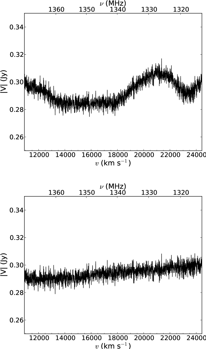
Figure 1: The visibility amplitude versus the Doppler corrected barycentric velocity, averaged over all epochs and array baselines, from the ATCA observations of J223931–360921. Top: Before removal of the spectral ripple. Bottom: After removal of the spectral ripple by subtracting a continuum model of other bright sources within the field of view. The spectral frequency is indicated on the upper abscissa; however it should be noted that the scale is linear only in velocity.

We construct data cubes from the flagged, calibrated and ripple-subtracted visibility data. We apply natural weighting to the visibilities in order to optimise the signal-to-noise in the image data. Each cube was constructed with 2 arcsec pixel resolution, in order to provide good sampling of the synthesised beam. The image data were deconvolved from the synthesised beam using the CLEAN algorithm, to produce images with a restoring beam FWHM of $10$ arcsec, typical of the maximum baseline distance. The target sources are mostly unresolved and so we extract the synthesised beam-weighted spectra from the 11 central pixels of each image plane. Fig. 2 displays 800 channels (equivalent to a velocity range of approximately 5600 km s^-1) of the extracted spectrum for each of the target sources, centred on the expected position of the 21 cm H i absorption line from optical redshift estimates. For the subsequent quantitative analysis presented here the central 1649 channels of the CABB zoom band are used, where 200 channels are flagged at each end of the band, to account for possible edge effects.

We estimate the standard deviation per spectral channel using the median of the absolute deviations from the median value (MADFM). This statistic is a more robust estimator of the true standard deviation than the rms when a strong signal is present in the data. Under the assumption of normal distributed data, the MADFM statistic ($\rho$) is related to the standard deviation ($\sigma$) by (Whiting, 2012)

$$\rho=\sqrt{2}\mathrm{erf}^{-1}(0.5)\sigma\approx 0.674\sigma,$$ (1)

and hence we can estimate the standard deviation in the spectral data by multiplying the MADFM statistic by a factor of 1.483. We calculate this statistic over the spectrum where we have subtracted the continuum and removed those channels that are expected to contain the spectral line. We assume that the standard deviation per channel is constant for the CABB data. Wilson et al. (2011) show that there is minimal overlap in the signal between the CABB spectral channels and so we assume that the uncertainty per channel is essentially uncorrelated in the subsequent analysis.

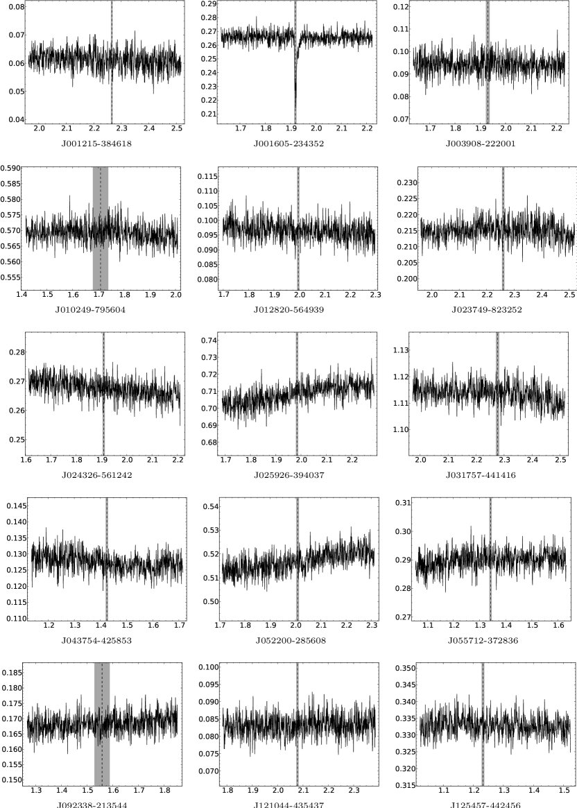
Figure 2: Synthesised beam-weighted spectra extracted from the position of each target source. For each spectrum the ordinate shows the synthesised beam-weighted flux (in Jy) and the abscissa the Doppler corrected barycentric velocity (in $10^{4}$ km s^-1). For clarity, only 800 of the 2049 CABB zoom band channels are displayed, centred near the optical redshift given in Table 1 (vertical dashed line). The grey region represents an estimate of the 1 $\sigma$ uncertainty in the optical redshift.

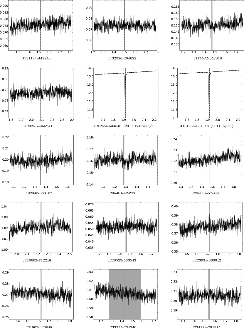
Figure 3: continued

3 Analysis

3.1 Bayesian inference

In the following analysis we adapt the method presented by Allison et al. (2011) in order to account for the relatively complex line-profiles expected in real spectral-line data from associated H i absorption. Analytical models are assumed for both the continuum and spectral-line components and simultaneously fit to the data using Bayesian inference.

The posterior (or joint) probability for a set of model parameters ($\boldsymbol{\theta}$), given the data ($\boldsymbol{d}$) and the model hypothesis ($\mathcal{M}$), can be calculated using Bayes’ Theorem,

$$\mathrm{Pr}(\boldsymbol{\theta}|\boldsymbol{d},\mathcal{M})={\mathrm{Pr}(\boldsymbol{d}|\boldsymbol{\theta},\mathcal{M})\mathrm{Pr}(\boldsymbol{\theta}|\mathcal{M})\over\mathrm{Pr}(\boldsymbol{d}|\mathcal{M})}.$$ (2)

The probability of the data given the set of model parameters, known as the likelihood, can be calculated based on assumptions about the distribution of the uncertainty in the data. If the data set is large and therefore quasi-continuous, one can approximate the likelihood by the form given for normal multivariate data (see e.g. Sivia, 2006),

$$L \equiv\mathrm{Pr}(\boldsymbol{d}|\boldsymbol{\theta},\mathcal{M})$$

$$={1\over\sqrt{(2\mathrm{\pi})^{N}|\mathbf{C}|}}\exp{\left[-{(\boldsymbol{d}-\boldsymbol{m})^{\mathrm{t}}\mathbf{C}^{-1}(\boldsymbol{d}-\boldsymbol{m})\over 2}\right]},$$ (3)

where $N$ is equal to the length of $\boldsymbol{d}$, $\mathbf{C}$ is the covariance matrix of the data, $|\mathbf{C}|$ is the determinant of the covariance matrix, and $\boldsymbol{m}$ is the vector of model data. In the special case where the uncertainty ($\sigma$) per datum is constant and uncorrelated, the above expression for the likelihood reduces to

$$L={1\over\sigma^{N}\sqrt{(2\mathrm{\pi})^{N}}}\exp{\left[-{1\over 2\sigma^{2}}\sum_{i=1}^{N}{(d_{i}-m_{i})^{2}}\right]}.$$ (4)

The probability of the model parameters given the hypothesis, $\mathrm{Pr}(\boldsymbol{\theta}|\mathcal{M})$, is known as the prior and encodes a priori information about the parameter values. For example, consider the situation where the frequency position of an intervening H i absorber has been relatively well constrained from previous observations. If we trust these observations we might then choose to apply a normal prior to the spectral line position based on the known level of uncertainty. We would otherwise apply uninformative priors to the parameters if we were previously unaware of their value. Uninformative priors are typically uniform in either linear space (for location parameters) or logarithmic space (for scale parameters, known as the Jeffreys prior).

The normalisation of the posterior probability in Equation 2 is equal to the probability of the data given the model hypothesis and is referred to throughout this work as the evidence. The evidence is calculated by marginalising the product of the likelihood and prior distributions over the model parameters. This is given by

$$E \equiv\mathrm{Pr}(\boldsymbol{d}|\mathcal{M})$$

$$=\int{\mathrm{Pr}(\boldsymbol{d}|\boldsymbol{\theta},\mathcal{M})\mathrm{Pr}(\boldsymbol{\theta}|\mathcal{M})\mathrm{d}\boldsymbol{\theta}},$$ (5)

which follows from the relation given by Equation 2 and that the integrated posterior is normalised to unity. When the model hypothesis provides a good fit to the data the likelihood peak will have a large value, and hence the model hypothesis will have a large associated evidence value. However if the model is over-complex then there will be large regions of low likelihood within the prior volume, thus reducing the evidence value for this model, in agreement with Occam’s razor. Estimation of the evidence is often key in providing a tool for selection between competing models.

3.2 Application to spectral data

We wish to investigate whether the spectral data warrant the inclusion of the spectral-line model in addition to the continuum model, and if so how many spectral-line components are favoured. The analytical expression for the continuum model is given by an $n_{\mathrm{poly}}$’th order polynomial of the form

$$S_{\mathrm{cont}}=S_{0}\left[1+\sum_{i=1}^{n_{\mathrm{poly}}}s_{i}\left({v\over v_{0}}-1\right)^{i}\right],$$ (6)

where $S_{\mathrm{cont}}$ is the model continuum flux density as a function of the Doppler corrected barycentric velocity $v$, $v_{0}$ is the fiducial velocity given by the first spectral channel (equal to approximately $1.16\times 10^{4}$ km s^-1 for the data presented here), $S_{0}$ is the spectral flux density at $v_{0}$ and, $s_{i}$ is the coefficient for the ith term. For the purposes of the work presented here we choose to use a 1st order polynomial (i.e. linear) model for the continuum component of the spectrum.

The spectral-line model is given by the sum over $n_{\mathrm{comp}}$ Gaussian components of the form

$$\Delta{S_{\mathrm{line}}}=\sum_{i=1}^{n_{\mathrm{comp}}}\Delta{S}_{i}\exp{\left[-4\ln(2){(v-v_{i})^{2}\over(\Delta{v}_{\mathrm{FWHM},i})^{2}}\right]},$$ (7)

where $\Delta{S}_{i}$ is the peak depth in flux density, $v_{i}$ is the velocity, and $\Delta{v}_{\mathrm{FWHM},i}$ is the FWHM of the ith component. The set of model data ($\boldsymbol{m}$) are calculated by taking the mean of the combined spectral model over each spectral channel. This assumes that the channel response of the CABB Filterbank Correlator is flat, which is a reasonable approximation for our purposes here (Wilson et al., 2011).

Table 2: Priors used in spectral-line detection. The model parameters are defined by Equations 6 and 7. $\langle{S_{\mathrm{obs}}}\rangle$ is the mean observed continuum flux density.

Parameter	Prior type	Prior range
$S_{0}$	Uniform	(0.1 – 10) $\times$ $\langle{S_{\mathrm{obs}}}\rangle$
$s_{1}$	Uniform	$\pm 1$
$v_{i}$	Uniform	min($v$) – max($v$)
$\Delta{v}_{\mathrm{FWHM},i}$	Uniform	0.1 – 104 km s-1
$\Delta{S}_{i}$	Uniform	(0 – 1) $\times$ $S_{0}$
Systematic Error	Normal	1 $\pm$ 0.01

We use uninformative priors for all of the parameters in our spectral model (see Table 2). The maximum value for the continuum normalisation $S_{0}$ is set by an estimate of the mean flux of the source. The line-depth prior on $\Delta{S}_{i}$ is set by the physical limit of the mean flux density of each source. The velocity position ($v_{i}$) is limited to within the range of velocities recorded in the data. The maximum velocity width ($\Delta{v}_{\mathrm{FWHM},i}$) of 10⁴  km s^-1 is considered to be a physically reasonable limit.

We use the following relationship for the relative probability of two hypotheses,

$${\mathrm{Pr}(\mathcal{M}_{1}|\boldsymbol{d})\over\mathrm{Pr}(\mathcal{M}_{2}|\boldsymbol{d})}={\mathrm{Pr}(\boldsymbol{d}|\mathcal{M}_{1})\over\mathrm{Pr}(\boldsymbol{d}|\mathcal{M}_{2})}{\mathrm{Pr}(\mathcal{M}_{1})\over\mathrm{Pr}(\mathcal{M}_{2})}={E_{1}\over E_{2}}{\mathrm{Pr}(\mathcal{M}_{1})\over\mathrm{Pr}(\mathcal{M}_{2})},\\$$ (8)

to quantify the relative significance of the combined spectral line & continuum model versus the continuum-only model. The ratio ${\mathrm{Pr}(\mathcal{M}_{1})/\mathrm{Pr}(\mathcal{M}_{2})}$ encodes our prior belief that one hypothesis is favoured over another. Since we assume no prior information on the presence of spectral lines, this ratio is equal to unity, and so the above selection criterion is then equal to the ratio of the evidences. We define the quantity

$$R\equiv\ln\left({E_{\mathrm{HI}}\over E_{\mathrm{cont}}}\right),$$ (9)

where $E_{\mathrm{HI}}$ is the evidence for the combined spectral line & continuum hypothesis and $E_{\mathrm{cont}}$ is the evidence for the continuum-only hypothesis. A value of $R$ greater than zero gives the level of significance for detection of the spectral line. A value of $R$ less than zero indicates that the data do not warrant the inclusion of a spectral-line component and so the detection is rejected.

3.3 Implementation

Table 3: The inferred values for model parameters from fitting a multiple Gaussian spectral-line model, where $n_{\mathrm{comp}}$ is the best-fitting number of components; $v_{i}$ is the component velocity; $\Delta{v}_{\mathrm{FWHM},i}$ is the FWHM; $\Delta{S}_{i}$ is the depth and $R$ is the natural logarithm of the ratio of probability for this model versus the no spectral-line model. Only target sources for which we detect H i absorption are shown.

AT20G name	$n_{\mathrm{comp}}$	$v_{i}$	$\Delta{v}_{\mathrm{FWHM},i}$	$\Delta{S}_{i}$	$R$
		(km s-1)	(km s-1)	(mJy)
J001605–234352	2	$19197.4\pm 1.8$	$64.5\pm 4.4$	$41.0\pm 2.8$	$535.3\pm 0.1$
		$19286\pm 14$	$138\pm 23$	$11.5\pm 1.5$
J181934–634548$a$	4	$19161.6\pm 0.6$	$46.0\pm 0.5$	$1812\pm 20$	$103157.2\pm 0.2$
		$19173.8\pm 2.4$	$212.5\pm 8.3$	$196.5\pm 8.3$
		$19182.6\pm 0.1$	$19.4\pm 0.4$	$1335\pm 32$
		$19331.6\pm 2.2$	$25.9\pm 7.5$	$102\pm 12$
J181934–634548$b$	4	$19162.9\pm 0.2$	$47.1\pm 0.3$	$1869\pm 15$	$211968.3\pm 0.2$
		$19179.1\pm 1.7$	$224.1\pm 5.0$	$175.0\pm 4.9$
		$19183.4\pm 0.1$	$19.4\pm 0.3$	$1288\pm 22$
		$19333.3\pm 0.8$	$18.8\pm 2.6$	$107.8\pm 9.2$
J205401–424238	1	$13048\pm 34$	$520\pm 140$	$4.5\pm 0.7$	$26.3\pm 0.1$

• Source observed in 2011 February.

• Source observed in 2011 April.

We fit our spectral model using the existing MultiNest package developed by Feroz & Hobson (2008) and Feroz, Hobson, & Bridges (2009). This software uses nested sampling (Skilling, 2004) to explore parameter space and robustly calculate both the posterior probability distribution and the evidence, for a given likelihood function and prior (provided by the user).

We first test for detection of the absorption line using a single component spectral-line model with multi-modal nested sampling, whereby samples are taken of multiple likelihood peaks within parameter space, thus allowing for the possibility of multiple absorption lines in the spectrum. For each peak in likelihood we calculate a local $E_{\mathrm{HI}}$ value for the single component model, and then compare it with $E_{\mathrm{cont}}$ for the continuum-only model. The significance of the combined spectral line & continuum model is inferred by the relative local value of $E_{\mathrm{HI}}$ compared with $E_{\mathrm{cont}}$. If the local value of $E_{\mathrm{HI}}$ is less than or equal to $E_{\mathrm{cont}}$ then this detection is rejected. Following the successful completion of the nested sampling algorithm, both the multi-modal local evidence values and the model parameter posterior probability are recorded.

For each detection obtained using the single component spectral-line model, we repeat the fitting process by iteratively increasing the number of components and comparing the values of $R$. This process continues until we optimize $R$ and we have found the best-fitting number of Gaussian components for the spectral line.

3.4 Systematic errors

We estimate an upper limit of 1 per cent for the calibration error in the CABB spectral data (Wilson et al., 2011). This is consistent with the difference in flux density (approximately $0.3$ per cent) for February and April observations of J181934–634548. We account for systematic errors introduced by imperfect band-pass, gain and flux-scale correction by introducing an additional parameter that multiplies the model spectral flux density. This nuisance parameter has a normal prior distribution with a mean value of unity and a standard deviation equal to 1 per cent, and is subsequently marginalised when calculating the posterior probability distributions for the model parameters.

3.5 Continuum residuals

When searching for H i absorption in real interferometric data we expect to obtain some false detections due to residual signal in the continuum that is not well fit by our continuum model. This could be due to imperfect spectral-ripple subtraction (see Section 2.2.2) or band-pass calibration. We expect that this problem will be worse for models with significantly large spectral-line widths and low depths, since at these values we would essentially be improving the continuum fit. The Bayesian method generates a marginalised posterior distribution for each model parameter, including the spectral-line width. We therefore inspect the line-width parameter a posteriori for unphysical values and potential association with a broad continuum residual. Since we are looking for associated absorption we can also reject those candidate broad detections with a line velocity that is very different to that predicted by existing optical redshift estimates.

Lastly we invert the spectrum and search for emission-like features, which could arise either from emission lines or continuum artefacts. We expect that a broad absorption-like ripple feature would likely be accompanied by an emission-like ripple feature. The residual contamination of spectra, both from spectral-ripple subtraction and imperfect band-pass calibration, will be of concern for future large field of view, wide-band H i absorption surveys. These surveys will require a reliable sky model for continuum subtraction.

4 Results and discussion

4.1 Observational results

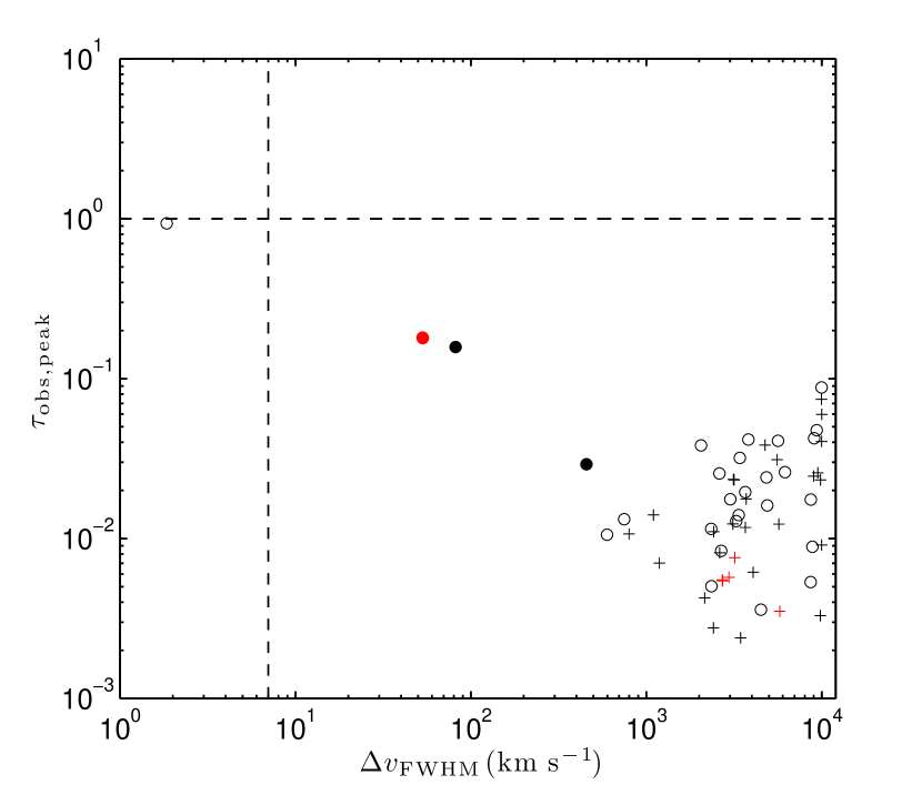
Figure 4: Best-fitting (maximum likelihood) values for the peak observed optical depth versus spectral-line width for absorption-like (circles) and emission-like (crosses) features detected using a single Gaussian model and multi-modal nested sampling. The filled circles are identified as H i absorption, while empty circles represent false detections. The red points represent features detected from observations of the brightest continuum source J181934–634548. The dashed lines indicate the position of the single channel width of 7 km s^-1 and an optical depth of $\tau=1$ respectively.

Fig. 4 summarizes both the absorption and emission features that were detected in data from all 29 target sources, using a single Gaussian spectral-line model and multi-modal nested sampling. It is evident from this plot that there is a significant number of identified false detections, clustered at broad spectral-line widths ($\Delta{v}_{\mathrm{FWHM}}\gtrsim 10^{3}$ km s^-1) and low peak optical depths ($\tau_{\mathrm{peak}}\lesssim 0.1$), as was discussed in Section 3.5. The probability distributions for some of these detections are peaked beyond the maximum prior for the spectral-line width ($10^{4}$ km s^-1) and so these points are shown at the limiting value. We obtain a total of 59 false detections, of which 30 are absorption-like and 29 are emission-like spectral features.

The false detections shown in Fig. 4 form a distinct grouping of broad, shallow features, which are clearly separate from the significant H i absorption detections in J001605–234352 and J181934–634548. The weaker detection seen in J205401–424238 has best-fitting values of peak observed optical depth and spectral-line width that are closer to those of the grouping of false detections. However it is the narrowest of the absorption-like features in this group ($\Delta{v}_{\mathrm{FWHM}}=520\pm 140$ km s^-1) and has a velocity that is consistent with that expected from the optical spectroscopic redshift. In total we have detected three associated H i absorption lines, of which two were previously unknown, giving a 10 per cent detection rate. Fig. 5 shows the optical and radio continuum images, and spectral model fitting results for the three sources with detected associated H i absorption. Table 3 summarizes the properties of the individual Gaussian components from model fitting.

The optical depth is related to the continuum flux density ($S_{\mathrm{cont}}$) and spectral-line depth ($\Delta{S_{\mathrm{line}}}$) by

$$\tau(v)=-\ln{\left(1-{\Delta{S_{\mathrm{line}}}\over fS_{\mathrm{cont}}}\right)},$$ (10)

where $f$ is the covering factor of the background source. Under the assumption that the absorption is optically thin ($\Delta{S_{\mathrm{line}}}/fS_{\mathrm{cont}}\lesssim 0.3$), the above expression for the optical depth reduces to

$$\tau(v)\approx{\Delta{S_{\mathrm{line}}}\over fS_{\mathrm{cont}}}\approx{\tau_{\mathrm{obs}}(v)\over f},$$ (11)

where $\tau_{\mathrm{obs}}(v)$ is the observed optical depth as a function of velocity. The H i column density (in cm^-2) is related to the integrated optical depth (in km s^-1) by (Wolfe & Burbidge, 1975)

$$N_{\mathrm{HI}} = 1.823\times 10^{18}\,T_{\mathrm{spin}}\int{\tau(v)\mathrm{d}v}$$ (12)

$$\approx 1.823\times 10^{18}\,{T_{\mathrm{spin}}\over f}\int{\tau_{\mathrm{obs}}(v)\mathrm{d}v},$$

where $T_{\mathrm{spin}}$ is the mean harmonic spin temperature of the gas (in K). Table 4 summarizes these quantities derived from model fitting.

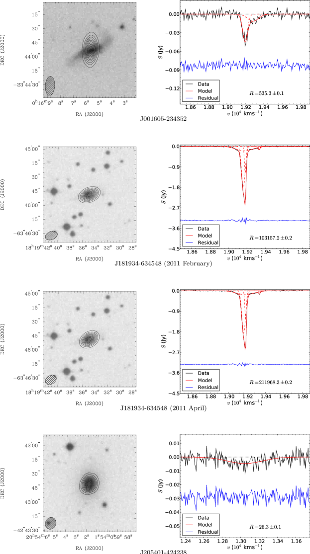
Figure 5: Target sources with detected H i absorption. Left: Images from the ATCA observations (contours) and the SuperCosmos Sky Survey (grey-scale; Hambly et al., 2001). The contours represent intervals of 10 per cent of the peak continuum brightness. The FWHM of the ATCA synthesised beam is displayed in the bottom left-hand corner of each image. Right: The corresponding spectra from the ATCA observations. The data have been simultaneously fit by a combined continuum and multiple Gaussian spectral-line model. The solid black line represents the data after subtraction of the best-fitting continuum component. The solid red line represents the best-fitting multiple Gaussian spectral-line model, and the dashed red lines represent individual components. The solid blue line represents the best-fitting residual, including a velocity-axis offset for clarity. $R$ refers to the detection significance as defined by Equation 9.

Table 4: A summary of derived H i absorption properties from model fitting, where $\sigma_{\mathrm{chan}}$ is the estimated uncertainty per channel; $S_{\mathrm{cont,peak}}$ is the spectral flux density of the continuum model at either the position of peak absorption or the optical redshift estimate; $\Delta{S}_{\mathrm{peak}}$ is the peak spectral-line depth; $\tau_{\mathrm{obs,peak}}$ is the observed peak optical depth and $\int{\tau_{\mathrm{obs}}\mathrm{d}v}$ is the observed velocity integrated optical depth. Upper limits are calculated assuming a single Gaussian spectral line of FWHM equal to 30 km s^-1 and peak depth equal to 3 $\sigma_{\mathrm{chan}}$.

AT20G name	$\sigma_{\mathrm{chan}}$	$S_{\mathrm{cont,peak}}$	$\Delta{S}_{\mathrm{peak}}$	$\tau_{\mathrm{obs,peak}}$	$\int{\tau_{\mathrm{obs}}\mathrm{d}v}$	$\log_{10}{\left(\mathrm{N}_{\mathrm{HI}}f\over T_{\mathrm{spin}}\right)}$
	(mJy)	(mJy)	(mJy)		(km s-1)
J001215–384618	3.53	60.9 $\pm$ 0.6	$<$ 10.6	$<$ 0.174	$<$ 5.55	$<$ 19.01
J001605–234352	3.71	265.8 $\pm$ 2.4	44.9 $\pm$ 1.8	0.169 $\pm$ 0.007	16.9 $\pm$ 0.7	19.49 $\pm$ 0.02
J003908–222001	4.20	94.5 $\pm$ 0.9	$<$ 12.6	$<$ 0.133	$<$ 4.26	$<$ 18.89
J010249–795604	2.97	568.9 $\pm$ 5.6	$<$ 8.9	$<$ 0.016	$<$ 0.50	$<$ 17.96
J012820–564939	3.29	96.4 $\pm$ 0.9	$<$ 9.9	$<$ 0.102	$<$ 3.27	$<$ 18.78
J023749–823252	2.89	215.2 $\pm$ 2.1	$<$ 8.7	$<$ 0.040	$<$ 1.28	$<$ 18.37
J024326–561242	3.26	267.5 $\pm$ 2.5	$<$ 9.78	$<$ 0.037	$<$ 1.17	$<$ 18.33
J025926–394037	4.93	708.4 $\pm$ 7.1	$<$ 14.8	$<$ 0.021	$<$ 0.67	$<$ 18.10
J031757–441416	3.73	1115 $\pm$ 10	$<$ 11.2	$<$ 0.010	$<$ 0.32	$<$ 17.77
J043754–425853	3.08	127.4 $\pm$ 1.3	$<$ 9.2	$<$ 0.072	$<$ 2.31	$<$ 18.63
J052200–285608	3.92	516.9 $\pm$ 4.9	$<$ 11.7	$<$ 0.023	$<$ 0.73	$<$ 18.12
J055712–372836	3.31	290.5 $\pm$ 2.7	$<$ 9.9	$<$ 0.034	$<$ 1.09	$<$ 18.30
J092338–213544	3.32	168.8 $\pm$ 1.6	$<$ 9.7	$<$ 0.059	$<$ 1.89	$<$ 18.53
J121044–435437	2.76	83.3 $\pm$ 0.8	$<$ 8.3	$<$ 0.099	$<$ 3.17	$<$ 18.76
J125457–442456	3.02	332.8 $\pm$ 3.1	$<$ 9.1	$<$ 0.027	$<$ 0.87	$<$ 18.20
J131124–442240	3.28	75.9 $\pm$ 0.8	$<$ 9.8	$<$ 0.130	$<$ 4.13	$<$ 18.88
J132920–264022	3.23	73.5 $\pm$ 0.7	$<$ 9.7	$<$ 0.132	$<$ 4.21	$<$ 18.88
J171522–652018	3.26	150.7 $\pm$ 1.5	$<$ 9.8	$<$ 0.065	$<$ 2.07	$<$ 18.58
J180957–455241	3.40	786.9 $\pm$ 7.0	$<$ 10.2	$<$ 0.013	$<$ 0.41	$<$ 17.88
J181934–634548$a$	12.55$c$	13709 $\pm$ 57	2632 $\pm$ 15	0.192 $\pm$ 0.001	11.92 $\pm$ 0.06	19.337 $\pm$ 0.002
J181934–634548$b$	8.87$c$	13754 $\pm$ 55	2654 $\pm$ 13	0.193 $\pm$ 0.001	11.93 $\pm$ 0.04	19.337 $\pm$ 0.001
J192043–383107	3.37	199.0 $\pm$ 1.9	$<$ 10.1	$<$ 0.051	$<$ 1.62	$<$ 18.47
J205401–424238	3.47	162.1 $\pm$ 1.5	4.5 $\pm$ 0.7	0.028 $\pm$ 0.004	13.4 $\pm$ 2.0	19.38 $\pm$ 0.07
J205837–575636	3.40	221.2 $\pm$ 2.1	$<$ 10.2	$<$ 0.046	$<$ 1.47	$<$ 18.43
J210602–712218	3.38	1021.9 $\pm$ 9.0	$<$ 10.2	$<$ 0.010	$<$ 0.32	$<$ 17.76
J220253–563543	3.23	51.8 $\pm$ 0.5	$<$ 9.7	$<$ 0.187	$<$ 5.98	$<$ 19.04
J223931–360912	4.22	377.8 $\pm$ 3.6	$<$ 12.7	$<$ 0.034	$<$ 1.07	$<$ 18.29
J231905–420648	3.42	270.7 $\pm$ 2.6	$<$ 10.3	$<$ 0.038	$<$ 1.21	$<$ 18.34
J233355–234340	4.47	606.2 $\pm$ 5.7	$<$ 13.4	$<$ 0.024	$<$ 0.71	$<$ 18.11
J234129–291915	4.11	204.9 $\pm$ 2.0	$<$ 12.3	$<$ 0.060	$<$ 1.92	$<$ 18.54

• Source observed in 2011 February.

• Source observed in 2011 April.

• Significantly higher per-channel variance due to band-pass calibrator.

4.2 Notes on individual sources

• We detect a previously unknown H i absorption feature with a peak observed optical depth of $0.169\pm 0.007$ and an integrated optical depth of $16.9\pm 0.7$ km s^-1. van Gorkom et al. (1989) include this source in their sample of radio galaxies with compact cores, observed using the Very Large Array. However, they do not include it in their search for 21 cm H i absorption since the unresolved continuum flux density (255 mJy) did not meet their selection criterion of greater than 350 mJy. The absorption line feature is best fit by two Gaussians, with a narrow component ($\Delta{v}_{\mathrm{FWHM}}=64.5\pm 4.4$ km s^-1), located at the spectroscopic optical redshift, and a single broad component ($\Delta{v}_{\mathrm{FWHM}}=138\pm 23$ km s^-1), which is slightly redshifted by $96\pm 46$ km s^-1. The host galaxy is classified as a blue spiral (UK Schmidt Telescope, Automated Photographic Measuring Bright Galaxy Catalogue; Loveday, 1996) located within the galaxy cluster Abell 14 (Savage & Wall, 1976; Dressler, 1980). Fig. 5 shows the blue optical image at the position of the target source (UK Schmidt Telescope, SuperCosmos Survey; Hambly et al., 2001), with an edge-on spiral galaxy that exhibits some disruption at the edges.

  Both the H i absorption line profile and the host morphology for this source demonstrate strong similarity with J181934–634548, studied at multiple wavelengths by Morganti et al. (2011). The narrow, deep absorption component is consistent with a gas-rich galactic disc, while the redshifted broad shallow component could be attributed to higher velocity gas close to the central AGN, perhaps in a circumnuclear disc. However to verify this interpretation we require further 21 cm observations at higher angular resolution (via long baseline interferometry).

• We obtain a low significance spectral-line feature ($R=4.26\pm 0.11$) at $z=0.0785\pm 0.0031$ with a width of $\Delta{v}_{\mathrm{FWHM}}=2.7\pm 1.2$ km s^-1. In Fig. 4 this feature is isolated to the very narrow spectral-line width and high optical depth region. This feature is redshifted by $4230\pm 930$ km s^-1 with respect to the systemic velocity, given by the spectroscopic optical redshift ($z=0.06438\pm 0.00025;$ Vettolani et al., 1989), and, if attributed to H i absorption, would likely represent an infall of gas at very high velocity. Because of this, and that the spectral-line width spans a single spectral channel, we suspect that this feature arises due to relatively high noise in this channel.

• This compact steep spectrum source (Tzioumis et al., 2002) has a previously known strong absorption feature (Véron-Cetty et al., 2000; Morganti et al., 2001) and was studied extensively at multiple wavelengths and angular scales by Morganti et al. (2011). In particular the host galaxy is known to have a strong edge-on disc morphology with heavily warped edges, consistent with recent merger activity. This is not easily apparent upon inspection of the blue optical image shown in Fig. 5, due to the presence of a bright coincident star.

  We re-detect the absorption feature in both of our February and April observations, with derived peak and integrated optical depths that are consistent within the error. We estimate a peak observed optical depth of $0.193\pm 0.001$ and an integrated optical depth of $11.92\pm 0.05$ km s^-1. The absorption line feature is best fit by four Gaussians, consisting of a deep, narrow component (combination of two Gaussians; $\Delta{v}_{\mathrm{FWHM}}\approx 20$ km s^-1 and $\Delta{v}_{\mathrm{FWHM}}\approx 50$ km s^-1), a shallow, broad component ($\Delta{v}_{\mathrm{FWHM}}\approx 200$ km s^-1), and a small redshifted component ($\Delta{v}_{\mathrm{FWHM}}\approx 20$ km s^-1). Of the two strong features, the broad component is slightly redshifted with respect to the narrow component, generating an asymmetry in the wings of the line profile towards the red end of the spectrum. Morganti et al. (2011) used observations with the Australian Long Baseline Array (LBA) to demonstrate that the absorption consists of a deep, narrow component from the edge-on disc of the galaxy, and a spatially resolved shallow, broad component from the cirumnuclear disc close to the radio source.

  In addition to these principle features we also detect a small component, which is redshifted from the systemic velocity by approximately 100 km s^-1, and has a peak optical depth $\approx 0.008$ and integrated optical depth $\approx 0.2$ km s^-1. The data from both of our February and April observations favour the inclusion of this additional Gaussian component, with the natural logarithm of the ratio of the probabilities of a 4-component to a 3-component model of $36.1\pm 0.2$ and $83.1\pm 0.2$ respectively. Inspection of the LBA spectrum obtained by Morganti et al. (2011) shows a similar feature, at this velocity, in the broad red-shifted wing of the profile seen against the northern lobe. It is therefore likely that this feature represents non-uniformity in the gas on the red-shifted side of the circumnuclear disc. A less likely interpretation, since the feature is only seen against the northern lobe, is that it indicates the presence of infall of gas towards the central AGN at a velocity greater than $100$ km s^-1.

• We detect a previously unknown H i absorption feature with a peak optical depth of $0.028\pm 0.004$ and an integrated optical depth of $13.4\pm 2.0$ km s^-1. This is the least significant of our three detections, however the single-component Gaussian fitting returns a significant relative log-probability of $26.3\pm 0.1$ for the spectral line hypothesis, and has a position that is consistent with the spectroscopic optical redshift. We note that this feature is apparent throughout the observation, in both polarisation feeds, and does not appear in spectra that are extracted from spatial positions significantly off the source. The single component is shallow and broad ($\Delta{v}_{\mathrm{FWHM}}=520\pm 140$ km s^-1) producing a relatively low peak, but high integrated, optical depth.

  The radio source is signified by a bright, flat spectrum, and was observed in the Combined Radio All-Sky Targeted Eight GHz Survey (CRATES; Healey et al., 2007). The host galaxy is classified as an elliptical by Loveday (1996), which is consistent with the optical image from the UK Schmidt Telescope shown in Fig. 5. That we detect only a single broad, shallow component at 21 cm suggests that we might be seeing only the absorption from gas close to the AGN, and nothing from the gas-poor elliptical host. Again in order to verify this interpretation we require further 21 cm observations at higher angular resolution (via long baseline interferometry).

4.3 Stacking for a statistical detection

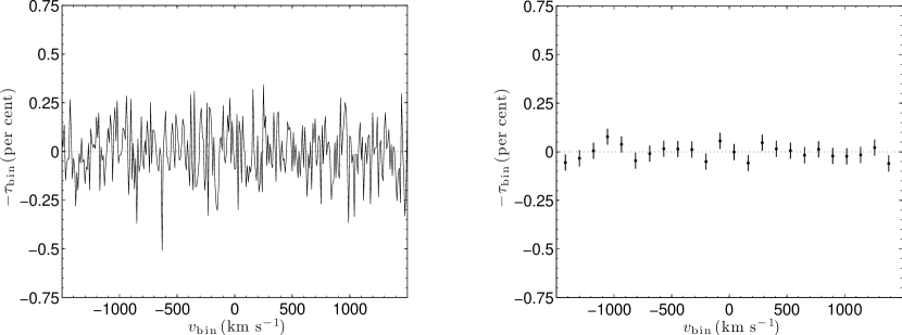
Figure 6: The binned optical depth spectra for the 26 sources with non-detections of H i absorption. The binned velocity axis is centred on the rest velocity given by the optical redshifts (see Table 1). A velocity range of $\pm$1500 km s^-1 is shown for clarity. Left: The data have been binned to 10 km s^-1, and so similar to the spectral resolution of the individual spectra. Right: The data have been binned to a resolution of 122 km s^-1, equal to the mean error in the optical spectroscopic redshift. The errorbars represent 1 $\sigma$.

While we do not detect H i absorption in 26 of the target sources with the ATCA, we can search for a statistical detection by stacking the individual spectra. For each spectrum we calculate the observed optical depth spectra, using the the best-fitting continuum model, and centre the velocity axis on the rest velocity, given by the optical spectroscopic redshift. We define the observed optical depth and weight, for the $j$ th datum, by

$$\tau_{j} = 1-{S_{j}\over S_{\mathrm{cont},j}},$$ (13)

$$w_{j} = \left(\sigma_{j}/S_{\mathrm{cont},j}\right)^{-2},$$ (14)

where $S_{j}$ is the spectral flux density, $S_{\mathrm{cont},j}$ is the best-fitting model continuum flux density and $\sigma_{j}$ is the uncertainty in $S_{j}$ . The binned optical depth ($\tau_{\mathrm{bin}}$), velocity ($v_{\mathrm{bin}}$) and uncertainty ($\sigma_{\mathrm{bin}}$) are then given by

$$\tau_{\mathrm{bin}} = \left[\sum_{j=1}^{n}{w_{j}\tau_{j}}\right]\left[\sum_{j=1}^{n}{w_{j}}\right]^{-1},$$ (15)

$$v_{\mathrm{bin}} = \left[\sum_{j=1}^{n}{w_{j}(v_{j}-cz_{\mathrm{opt},j})}\right]\left[\sum_{j=1}^{n}{w_{j}}\right]^{-1},$$ (16)

$$\sigma_{\mathrm{bin}} = \left[\sum_{j=1}^{n}{w_{j}}\right]^{-1/2},$$ (17)

where $v_{j}$ and $z_{\mathrm{opt},j}$ are the spectral velocity and optical spectroscopic redshift respectively. Fig. 6 shows the binned flux density versus velocity for the stacked non-detections. We consider two values for the velocity bin widths, in one case similar to the spectral resolution of an individual spectrum and the second case equal to the mean uncertainty in the optical spectroscopic redshift ($\approx 122$ km s^-1), and hence approximately equal to the smearing scale for any spectral line. The optical depth sensitivity for the narrow-binned spectrum is 0.14 per cent. Using the spectral-line finding method outlined in Section 3, with a normal prior on the spectral-line velocity of $v=0\pm 122$ km s^-1, we find that there is no evidence of a statistical detection of 21 cm associated H i absorption in the stacked non-detections.

4.4 Intervening H I absorption

Based on both the lower redshift limit available from our observations ($z_{\mathrm{min}}=0.0338$) and the optical spectroscopic redshifts of the 29 target sources, the total redshift path searched for potential intervening H i absorption is $\Delta{z}_{\mathrm{total}}\approx 0.6093$, assuming that there is no high-velocity, redshifted intervening gas towards our sources. We can estimate the expected number of high column density intervening H i absorbers in this redshift path from previous work on nearby galaxies. Zwaan et al. (2005) used 21 cm line observations of 355 nearby galaxies in the Westerbork H i survey of Spiral and Irregular galaxies (WHISP; van der Hulst, van Albada, & Sancisi 2001) to estimate the number density of damped Lyman-$\alpha$ galaxies (DLAs, defined by $N_{\mathrm{HI}}>2\times 10^{20}$ cm^-2) at $z=0$. Based on their estimate of $\mathrm{d}N/\mathrm{d}z=0.045\pm 0.006$, and assuming no strong evolution over our redshift range, we would expect to find approximately 0.027 DLAs within our total redshift search path (assuming no a priori information of the location of foreground galaxies). If we assume that $T_{\mathrm{spin}}/f=100$ K, then a single DLA equates to an observed integrated optical depth of 1.09 km s^-1, which is comparable to the mean sensitivity of our sample of 1.85 km s^-1. It is therefore highly unlikely that we would have detected intervening H i absorption in our sample, and that we could have confused one of these systems with a continuum residual signal (which would also require a significantly broad spectral-line width for the absorption). It should also be noted that this result does not change significantly if we use a different estimate for the low redshift number density, for example $\mathrm{d}N/\mathrm{d}z=0.046^{+0.03}_{-0.02}$ (Ryan-Weber, Webster, & Staveley-Smith, 2003) or $\mathrm{d}N/\mathrm{d}z=0.026\pm 0.003$ (Braun, 2012).

4.5 Detection rate for associated H I absorption

4.5.1 Comparison with other surveys

Table 5: A comparison with other similar surveys of associated H i absorption. $N_{\mathrm{obs}}$ is the total number of target sources; $N_{\mathrm{det}}$ is the number of H i absorption detections and $N_{0.05}$ is the number of detections with observed peak optical depth greater than 0.05.

Ref.	Telescope	$z$ range	$N_{\mathrm{obs}}$	$N_{\mathrm{det}}$	Rate	$N_{\mathrm{0.05}}$	Targets
					(per cent)
van Gorkom et al. 1989	VLA	0.004 – 0.128	29	4	14	1	Compact cores of E/S0 galaxies
Morganti et al. 2001	VLA/ATCA	0.011 – 0.220	23	5	22	2	Radio galaxies selected at 2.7 GHz
Vermeulen et al. 2003	WSRT	0.198 – 0.842	57	19	33	2	Compact radio sources
Orienti et al. 2006	WSRT	0.021 – 0.668	6	2	33	1	High-frequency peaker radio galaxies
Gupta et al. 2006	Arecibo/GMRT	0.016 – 1.311	27	6	22	1	GPS and CSS radio sources
Emonts et al. 2010	VLA/WSRT	0.002 – 0.044	23	6	26	3	Low luminosity radio sources (compact and FR-i)
Chandola et al. 2011	GMRT	0.024 – 0.152	18	7	39	3	GPS and CSS radio sources (CORALZ)
This work	ATCA	0.041 – 0.076	29	3	10	2	AT20G radio sources selected at 20 GHz

Table 5 compares our results with those of other similar associated H i absorption line studies that preferentially target compact objects. The total detection rate for our survey (10 per cent) is the lowest out of these studies, and comparable to the survey of compact cores of E and S0 galaxies by van Gorkom et al. (1989). Fig. 7 shows the observed integrated optical depth versus the 1.4 GHz flux density, for all the associated H i absorption surveys listed in Table 5 and the $z>0.1$ sample discussed by Curran et al. (2011). From this plot it is evident that the majority of our sample have relatively low fluxes and so our observations are typically sensitive to a higher observed integrated optical depth limit than the other surveys. This is a possible reason for the relatively low detection rate obtained in this work, indeed if one only counts detections with an observed peak optical depth greater than 0.05 then this number is comparable to the other surveys (albeit with large uncertainty due to low-number statistics). However there are potential errors associated with this interpretation, since some of our observations are sensitive to observed optical depths much less than 0.05 (see Table 4) and there are some high integrated optical depth detections seen in the lower flux sources (Fig. 7). We also note that the observed optical depth upper limits are based on simple assumptions about the underlying spectral-line width and depth.

4.5.2 Ultra-violet luminosity

A low detection rate of associated H i absorption in high redshift sources was found by Curran et al. (2008), who obtained no detections from the 13 ($z\gtrsim 3$) radio galaxies and quasars searched. Upon a detailed analysis of the photometry of the objects, all of the targets were found to have ultra-violet luminosities greater than an apparently critical value ($L_{1216}\sim 10^{23}$ W Hz^-1) at $\lambda=1216$ Å, above which the photon energy is sufficient to excite the hydrogen atom above the ground state and close to ionisation. Curran et al. (2008) therefore attributed the low detection rate to the high redshift selection of the targets biasing towards the most ultra-violet luminous objects. In further work by Curran et al. (2011) it was found that there are no detections of H i absorption in the known 19 target sources with $L_{1216}>10^{23}$ W Hz^-1. Assuming a 50 per cent detection rate (see Curran & Whiting, 2010) this distribution has a binomial probability of $9.5\times 10^{-7}$ of occuring by chance.

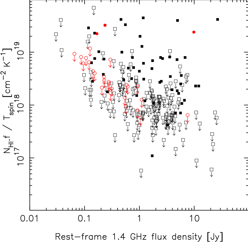
Figure 7: The normalised H i column density ($1.823\times 10^{18}\int{\tau_{\mathrm{obs}}\mathrm{d}v}$) versus the rest-frame 1.4 GHz flux density for the radio galaxies and quasars searched in 21 cm associated H i absorption. The filled symbols represent the 21 cm detections and the unfilled symbols the non-detections. The squares show results from previous searches (Table 5 and Curran et al. 2011) with the circles designating the sources presented here.

Fig. 8 shows the estimated ultra-violet luminosity, at a rest wavelength of $\lambda=1216$ Å, for all the associated H i absorption surveys. Most of our target sample (24 sources) have measured fluxes from the Galaxy Evolution Explorer (GALEX; Martin et al., 2003), with the remaining each having several flux measurements at rest-frame frequencies of $\nu\gtrsim 10^{14}$ Hz, thus allowing us to determine the luminosity at $2.47\times 10^{15}$ Hz. However only one of the sources has $L_{1216}\gtrsim 10^{22}$ W Hz^-1; J171522–652018 with $\log_{10}(L_{1216})\approx 22.7$. This is one of the three sources for which there is no photometry at $\nu\gtrsim 10^{15}$ Hz and so the estimated ultra-violet luminosity is unreliable. Therefore the low detection rate of our survey cannot be explained by the same extreme ultra-violet luminosities introduced by selecting a high redshift sample.

4.5.3 Radio luminosity

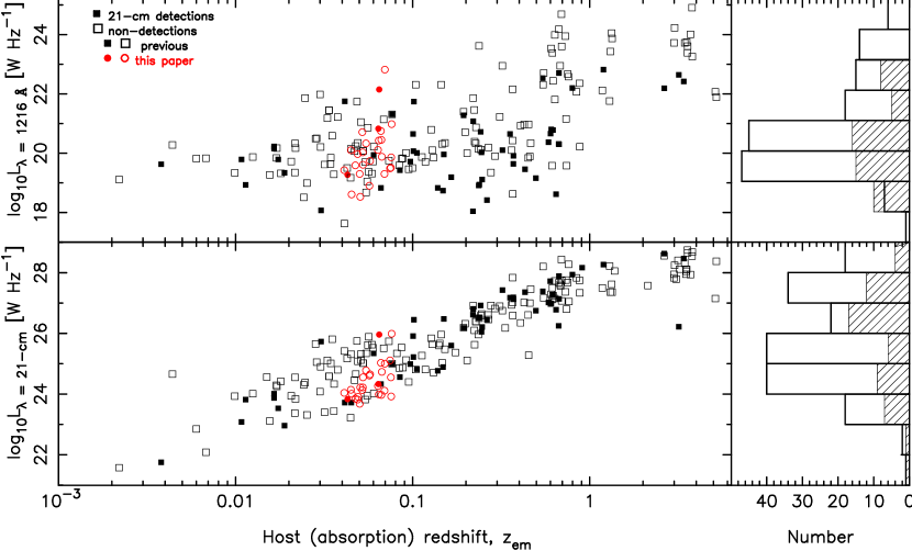
Figure 8: The rest-frame $\lambda=1216$ Å continuum luminosity (top) and 21 cm continuum luminosity (bottom) versus the host redshift for the radio galaxies and quasars searched in 21 cm associated H i absorption. The filled symbols/hatched histogram represent the 21 cm detections and the unfilled symbols/unfilled histogram the non-detections. The squares show results from previous searches (Table 5 and Curran et al., 2011) with the circles designating the sources presented here.

Fig. 8 also shows the estimated radio luminosity, at a rest wavelength of $\lambda$ = 21 cm, for all the associated H i absorption surveys. Not suprisingly, given target source selection, there is an apparent strong correlation between the radio luminosity and the redshift (17 $\sigma$). It is evident from this plot that the total detection rate for H i absorption is higher at $L_{\mathrm{21\,cm}}\gtrsim 10^{26}$ W Hz^-1 (30.8 per cent, versus 19.2 per cent at lower luminosities). The target sources in our sample have radio luminosities of $L_{\mathrm{21\,cm}}\lesssim 10^{26}$ W Hz^-1, and so the lower detection rate in our sample might be consistent with that expected for these sources. We note that the data shown in Fig. 7 also include observations by Emonts et al. (2010), who conducted a survey of nearby low luminosity radio galaxies ($22<\log_{10}(L_{\mathrm{21\,cm}})<25$ W Hz^-1), and obtained a relatively high detection rate of 6 (26 per cent) out of a sample of 23 sources. However, because all of these H i absorption systems were found to be associated with the host galaxy’s large-scale interstellar medium (ISM), their sample may be biased against intrinsically weak sources that are confined by the surrounding gas. Given the selection effects and small number of targets associated with existing HI absorption surveys, it is difficult to compare and interpret their individual detection rates. For this, future proposed large-scale surveys, such as FLASH (see Section 1) will be crucial.

Given the apparent higher total detection rate for H i absorption in higher radio luminosity sources, we might speculate that there is a correlation between the neutral hydrogen column density of the host and the radio luminosity of the source. For example Chandola et al. (2011) searched for a correlation between the neutral hydrogen column density and 5 GHz radio luminosity, both in the Compact Radio sources at Low Redshift sample (CORALZ; Snellen et al., 2004) and the survey by Gupta et al. (2006), and found no statistically significant evidence. However, since the neutral hydrogen column density is derived from an assumed $T_{\mathrm{spin}}/f$, it is possible that higher spin temperatures in the most radio luminous sources nullify any underlying relationship. If so then we might expect to see a limiting radio luminosity above which no detections are obtained, similar to that seen for the ultra-violet luminosity. This was tested by Curran & Whiting (2010) who found no significant evidence for such a limiting radio luminosity value.

4.5.4 Compact sources

When selecting our AT20G candidate sources for observation, priority was given to objects that did not exhibit extended emission, both at 20 GHz and in the lower frequency NVSS (1.4 GHz) and SUMSS (843 MHz) images. The motivation to preferentially select young and compact sources was based on previous work, which claims a significantly higher detection rate in compact sources (see Section 1). Given these results we might conclude that the compact sources either have intrinsically higher neutral hydrogen column densities (e.g. Pihlström et al., 2003) or that the flux density of the background continuum source is concentrated behind the absorbing gas, boosting the covering factor $f$.

However Curran & Whiting (2010) showed that when the $L_{1216}>10^{23}$ W Hz^-1 sources were removed from the sample, the 21 cm detection rate in compact sources was not significantly higher than that for non-compact sources. The elevated detection rate in compact sources was therefore interpreted as these having apparently lower ultra-violet luminosities, consistent with the hypothesis that these are young objects. In Fig. 9 we update the results of Curran & Whiting (2010) to include the work presented here and more recent results (including Emonts et al., 2010; Curran et al., 2011; Chandola et al., 2011). This figure shows the total number of detections and non-detections for sources classified as compact (either compact symmetric object – CSO, compact steep spectrum – CSS, gigahertz peaked spectrum – GPS or high frequency peaker – HPF), compared with those that are non-compact or unclassified. While the total number of detections is greatest for the compact sources we note that there is also a significant number of non-detections. The detection rates for each classification, for the whole sample, are 32.7 per cent (compact) versus 18.6 per cent (other) and 16.1 per cent (unclassified). For the sub-sample of sources with $L_{1216}\leq 10^{23}$ W Hz^-1, the detection rates are 33.9 per cent (compact) versus 23.5 per cent (other) and 18.2 per cent (unclassified). Therefore the detection rate is slighty higher for the compact sources, although not significantly so if we only consider the sub-sample of sources with $L_{1216}\leq 10^{23}$ W Hz^-1.

Figure 9: The incidence of detections (hatched histogram) and non-detections (unfilled histogram) for compact objects (CSO, CSS, GPS and HFP), compared to the others (non-compact and unclassified). Top: the whole sample (Table 5 and Curran et al., 2011). Bottom: those with $L_{1216}\leq 10^{23}$ W Hz^-1.

5 Summary

We have conducted a search for 21 cm associated H i absorption towards 29 target sources from the AT20G catalogue (Murphy et al., 2010), within the redshift range $0.04\lesssim z\lesssim 0.08$ and at a velocity resolution of 7 km s^-1. Since these sources are selected at high frequency, they are expected to be relatively young and represent the most recently-triggered radio AGN. We detect three associated absorption systems, of which two were previously unknown, yielding a 10 per cent detection rate. This detection rate is consistent with that seen for previous target sources at similar radio luminosities, and perhaps given the typical optical depth sensitivity of our survey. However these interpretations should be treated with caution until we have obtained significantly larger sample sizes from future large-scale surveys (e.g. ASKAP-FLASH with a proposed $\sim 150,000$ lines-of-sight).

Of the three detected H i absorption lines, two exhibit separate broad, shallow and narrow, deep components, while the third consists of a single broad, shallow component. These separate components are attributed to the relative orientation of both a galactic disc (low velocity gas) and a circumnuclear disc (high velocity gas) with respect to the line-of-sight (e.g. Morganti et al., 2011). In future work we aim to follow up the 2 previously unknown detections with long baseline interferometric observations, in order to spatially resolve the component features.

Our search for associated H i absorption in this sample was aided by a method of detection using Bayesian inference, developed by Allison et al. (2011) for the ASKAP FLASH survey, to both detect absorption and obtain the best-fitting number of components of the spectral-line profile. While this method is a powerful tool for performing automated searches of spectral lines in low signal-to-noise data, we must be wary of the limitations produced by other signals that contaminate the continuum. In particular it seems that for non-ideal band-pass calibration and continuum subtraction there will exist in the spectral data continuum residuals that look like broad, shallow spectral lines. For targeted associated absorption studies we are fortunate that we have a priori information on the expected spectral-line velocity from measured optical redshifts. However in the case of future large-scale blind surveys for both intervening and associated absorption it will be vitally important to have good calibration of the band-pass and simultaneous accurate models of the continuum sky. We note that by studying the posterior distribution of the model parameters, produced by the Bayesian inference method, we can filter out those detections that do not meet pre-selected physically-motivated criteria, such as a given parameter space of spectral-line width, depth and velocity. Further targeted study of H i absorption systems will allow us to improve these criteria.

References

- Allison et al. (2011) Allison J. R., Sadler E. M., Whiting M. T., 2011, Publ. Astron. Soc. Australia, in press, preprint (arXiv:1109.3539)
- Baldi & Capetti (2009) Baldi R. D., Capetti A., 2009, A&A, 508, 603
- Braun (2012) Braun R., 2012, ApJ, 749, 87
- Chandola et al. (2011) Chandola Y., Sirothia S. K., Saikia D. J., 2011, MNRAS, 418, 1787
- Colless et al. (2003) Colless M. et al., 2003, preprint (arXiv:astro-ph/0306581)
- Condon et al. (1998) Condon J. J., Cotton W. D., Greisen E. W., Yin Q. F., Perley R. A., Taylor G. B., Broderick J. J., 1998, AJ, 115, 1693
- Croton et al. (2006) Croton D. J. et al., 2006, MNRAS, 365, 11
- Curran et al. (2009) Curran S., Whiting M., Webb J., 2009, in Panoramic Radio Astronomy: Wide-field 1-2 GHz Research on Galaxy Evolution, Heald, G. & Serra, P., ed., Proc. Sci.
- Curran & Whiting (2010) Curran S. J., Whiting M. T., 2010, ApJ, 712, 303
- Curran & Whiting (2012) Curran S. J., Whiting M. T., 2012, preprint (arXiv:1204.2881)
- Curran et al. (2011) Curran S. J. et al., 2011, MNRAS, 413, 1165
- Curran et al. (2008) Curran S. J., Whiting M. T., Wiklind T., Webb J. K., Murphy M. T., Purcell C. R., 2008, MNRAS, 391, 765
- Deboer et al. (2009) Deboer D. R. et al., 2009, Proc. IEEE, 97, 1507
- Dressler (1980) Dressler A., 1980, ApJS, 42, 565
- Drinkwater et al. (2001) Drinkwater M. J., Gregg M. D., Holman B. A., Brown M. J. I., 2001, MNRAS, 326, 1076
- Emonts et al. (2010) Emonts B. H. C. et al., 2010, MNRAS, 406, 987
- Fanaroff & Riley (1974) Fanaroff B. L., Riley J. M., 1974, MNRAS, 167, 31P
- Feroz & Hobson (2008) Feroz F., Hobson M. P., 2008, MNRAS, 384, 449
- Feroz et al. (2009) Feroz F., Hobson M. P., Bridges M., 2009, MNRAS, 398, 1601
- Ghisellini (2011) Ghisellini G., 2011, in AIP Conf. Ser., Vol. 1381, 25th Texas Symposium on Relativistic Astrophysics, Aharonian, F. A., Hofmann, W. & Rieger F. M., ed., Am. Inst. Phys., New York, p. 180
- Gupta et al. (2006) Gupta N., Salter C. J., Saikia D. J., Ghosh T., Jeyakumar S., 2006, MNRAS, 373, 972
- Hambly et al. (2001) Hambly N. C. et al., 2001, MNRAS, 326, 1279
- Healey et al. (2007) Healey S. E., Romani R. W., Taylor G. B., Sadler E. M., Ricci R., Murphy T., Ulvestad J. S., Winn J. N., 2007, ApJS, 171, 61
- Högbom (1974) Högbom J. A., 1974, A&AS, 15, 417
- Holt et al. (2008) Holt J., Tadhunter C. N., Morganti R., 2008, MNRAS, 387, 639
- Jackson et al. (2002) Jackson C. A., Wall J. V., Shaver P. A., Kellermann K. I., Hook I. M., Hawkins M. R. S., 2002, A&A, 386, 97
- Jauncey et al. (1978) Jauncey D. L., Wright A. E., Peterson B. A., Condon J. J., 1978, ApJL, 219, L1
- Jones et al. (2009) Jones D. H. et al., 2009, MNRAS, 399, 683
- Katgert et al. (1998) Katgert P., Mazure A., den Hartog R., Adami C., Biviano A., Perea J., 1998, A&AS, 129, 399
- Loveday (1996) Loveday J., 1996, MNRAS, 278, 1025
- Mahony et al. (2011) Mahony E. K. et al., 2011, MNRAS, 417, 2651
- Martin et al. (2003) Martin C. et al., 2003, Proc. SPIE, 4854, 336
- Massardi et al. (2011) Massardi M. et al., 2011, MNRAS, 412, 318
- Mauch et al. (2003) Mauch T., Murphy T., Buttery H. J., Curran J., Hunstead R. W., Piestrzynski B., Robertson J. G., Sadler E. M., 2003, MNRAS, 342, 1117
- Morganti et al. (2011) Morganti R., Holt J., Tadhunter C., Ramos Almeida C., Dicken D., Inskip K., Oosterloo T., Tzioumis T., 2011, A&A, 535, A97
- Morganti et al. (1999) Morganti R., Oosterloo T., Tadhunter C. N., Aiudi R., Jones P., Villar-Martin M., 1999, A&AS, 140, 355
- Morganti et al. (2001) Morganti R., Oosterloo T. A., Tadhunter C. N., van Moorsel G., Killeen N., Wills K. A., 2001, MNRAS, 323, 331
- Morganti et al. (2005) Morganti R., Tadhunter C. N., Oosterloo T. A., 2005, A&A, 444, L9
- Murphy et al. (2010) Murphy T. et al., 2010, MNRAS, 402, 2403
- Orienti et al. (2006) Orienti M., Morganti R., Dallacasa D., 2006, A&A, 457, 531
- Peterson et al. (1979) Peterson B. A., Wright A. E., Jauncey D. L., Condon J. J., 1979, ApJ, 232, 400
- Pihlström et al. (2003) Pihlström Y. M., Conway J. E., Vermeulen R. C., 2003, A&A, 404, 871
- Ryan-Weber et al. (2003) Ryan-Weber E. V., Webster R. L., Staveley-Smith L., 2003, MNRAS, 343, 1195
- Sault et al. (1995) Sault R. J., Teuben P. J., Wright M. C. H., 1995, in ASP Conf. Ser., Vol. 77, Astronomical Data Analysis Software and Systems IV, Shaw R. A., Payne H. E., & Hayes J. J. E., ed., Astron. Soc. Pac., San Francisco, p. 433
- Savage & Wall (1976) Savage A., Wall J. V., 1976, Australian J. Phys. Astrophys. Suppl., 39, 39
- Simpson et al. (1993) Simpson C., Clements D. L., Rawlings S., Ward M., 1993, MNRAS, 262, 889
- Sivia (2006) Sivia D. S., 2006, Data Analysis: A Bayesian Tutorial., 2nd edn. Oxford University Press, New York
- Skilling (2004) Skilling J., 2004, in AIP Conf. Ser., Vol. 735, Bayesian Inference and Maximum Entropy methods in Science and Engineering, Fischer R., Preuss R. & Toussaint U. V., ed., Am. Inst. Phys., New York, p. 395
- Skrutskie et al. (2006) Skrutskie M. F. et al., 2006, AJ, 131, 1163
- Smith et al. (2004) Smith R. J. et al., 2004, AJ, 128, 1558
- Snellen et al. (2004) Snellen I. A. G., Mack K.-H., Schilizzi R. T., Tschager W., 2004, MNRAS, 348, 227
- Srianand et al. (2010) Srianand R., Gupta N., Petitjean P., Noterdaeme P., Ledoux C., 2010, MNRAS, 405, 1888
- Tzioumis et al. (2002) Tzioumis A. et al., 2002, A&A, 392, 841
- van der Hulst et al. (2001) van der Hulst J. M., van Albada T. S., Sancisi R., 2001, in ASP Conf. Ser., Vol. 240, Gas and Galaxy Evolution, Hibbard J. E., Rupen M., & van Gorkom J. H., ed., Astron. Soc. Pac., San Francisco, p. 451
- van Gorkom et al. (1989) van Gorkom J. H., Knapp G. R., Ekers R. D., Ekers D. D., Laing R. A., Polk K. S., 1989, AJ, 97, 708
- Vermeulen et al. (2003) Vermeulen R. C. et al., 2003, A&A, 404, 861
- Véron-Cetty et al. (2000) Véron-Cetty M.-P., Woltjer L., Staveley-Smith L., Ekers R. D., 2000, A&A, 362, 426
- Vettolani et al. (1989) Vettolani G., Cappi A., Chincarini G., Focardi P., Garilli B., Gregorini L., Maccagni D., 1989, A&AS, 79, 147
- Whiting (2012) Whiting M. T., 2012, MNRAS, 421, 3242
- Wills & Wills (1976) Wills D., Wills B. J., 1976, ApJS, 31, 143
- Wilson et al. (2011) Wilson W. E. et al., 2011, MNRAS, 416, 832
- Wolfe & Burbidge (1975) Wolfe A. M., Burbidge G. R., 1975, ApJ, 200, 548
- Zwaan et al. (2005) Zwaan M. A., van der Hulst J. M., Briggs F. H., Verheijen M. A. W., Ryan-Weber E. V., 2005, MNRAS, 364, 1467