Compton Scattering of Self-Absorbed Synchrotron Emission

Abstract

Synchrotron self-Compton (SSC) scattering is an important emission mechanism in many astronomical sources, such as gamma-ray bursts (GRBs) and active galactic nuclei (AGNs). We give a complete presentation of the analytical approximations for the Compton scattering of synchrotron emission with both weak and strong synchrotron self-absorption. All possible orders of the characteristic synchrotron spectral breaks ($\nu_{\rm a}$, $\nu_{\rm m}$, and $\nu_{\rm c}$) are studied. In the weak self-absorption regime, i.e., $\nu_{\rm a}<\nu_{c}$, the electron energy distribution is not modified by the self-absorption process. The shape of the SSC component broadly resembles that of synchrotron, but with the following features: The SSC flux increases linearly with frequency up to the SSC break frequency corresponding to the self-absorption frequency $\nu_{\rm a}$; and the presence of a logarithmic term in the high-frequency range of the SSC spectra makes it harder than the power-law approximation. In the strong absorption regime, i.e. $\nu_{\rm a}>\nu_{\rm c}$, heating of low energy electrons due to synchrotron absorption leads to pile-up of electrons, and form a thermal component besides the broken power-law component. This leads to two-component (thermal + non-thermal) spectra for both the synchrotron and SSC spectral components. For $\nu_{\rm c}<\nu_{\rm a}<\nu_{\rm m}$, the spectrum is thermal (non-thermal) -dominated if $\nu_{a}>\sqrt{\nu_{m}\nu_{c}}$ ($\nu_{a}<\sqrt{\nu_{m}\nu_{c}}$). Similar to the weak-absorption regime, the SSC spectral component is broader than the simple broken power law approximation. We derive the critical condition for strong absorption (electron pile-up), and discuss a case of GRB reverse shock emission in a wind medium, which invokes $\nu_{\rm a}>{\rm max}(\nu_{\rm m},\nu_{\rm c})$.

1 Introduction

Astrophysical sources powered by synchrotron radiation should have a synchrotron self-Compton (SSC) scattering component. The same electrons that radiate synchrotron photons would scatter these synchrotron seed photons to high energies, forming a distinct spectral component. The SSC mechanism has been invoked to account for the observed high energy emission in many astrophysical sources, such as gamma-ray bursts (GRBs) (e.g. Mészáros et al., 1994; Wei & Lu, 1998; Dermer et al., 2000; Panaitescu & Kumar, 2000; Sari & Esin, 2001; Zhang & Mészáros, 2001; Wang et al., 2001; Wu et al., 2004; Zou et al., 2009) and active galactic nuclei (AGNs) (e.g. Ghisellini et al., 1998b; Chiang & Böttcher, 2002; Zhang et al., 2012).

SSC is a complex process. The flux at each observed frequency includes the contributions from electrons in a wide range of energies, which scatter seed photons in a wide range of frequencies. Therefore, a precise description of the SSC spectrum invokes a complex convolution of the seed photon spectrum and electron energy distribution, which requires numerical calculations. However, for a synchrotron source with shock-accelerated electrons, the injected electron spectrum is usually assumed to be a simple power-law function, the corresponding electron energy distribution and seed synchrotron spectrum thus have simple patterns. Some analytical approximations for the SSC spectrum can be then made if Compton scattering is in the Thomson regime.

Besides the injected electron spectrum, two other factors are essential to define the shape of the final electron energy distribution in a synchrotron source: radiation cooling and self-absorption heating. There are three characteristic synchrotron frequencies in the spectrum: the minimum injection frequency ($\nu_{\rm m}$), the cooling frequency ($\nu_{c}$), and the self-absorption frequency ($\nu_{\rm a}$). When $\nu_{\rm a}<\nu_{\rm c}$, the heating effect due to self-absorption is not important in modifying the electron energy spectrum. For a continuous injection of a power-law electron spectrum, the final electron energy distribution is a broken power law. The seed synchrotron spectrum for SSC is characterized by a multi-segment broken power law, separated by $\nu_{m}$, $\nu_{c}$, and $\nu_{a}$. Different ordering of the three characteristic frequencies leads to different shapes of the seed synchrotron spectrum. In the literature, usually $\nu_{\rm a}<{\rm min}(\nu_{\rm m},\nu_{\rm c})$ is assumed. Sari & Esin (2001) have derived the approximated expressions of the SSC spectrum in the $\nu_{\rm a}<\nu_{\rm m}<\nu_{\rm c}$ and $\nu_{\rm a}<\nu_{\rm c}<\nu_{\rm m}$ regimes, respectively.

When $\nu_{\rm a}>\nu_{\rm c}$, synchrotron self-absorption becomes an important heating source for the low-energy electrons. Consequently, the electrons are dominated by a quasi-thermal component until a “transition” Lorentz factor $\gamma_{\rm t}$, above which the electrons are no longer affected by the self-absorption heating and keep the normal power law distribution (Ghisellini et al., 1988, 1991, 1998a). For these strong absorption cases, a thermal peak due to pile-up electrons would appear around $\nu_{\rm a}$ in the synchrotron spectrum (Kobayashi et al., 2004), which would also result in some new features in the SSC spectrum.

In this paper, we extend the analysis of Sari & Esin (2001) and present the full analytical approximated expressions of the SSC spectrum in all six possible cases of $\nu_{\rm a}$, $\nu_{\rm m}$, $\nu_{\rm c}$ ordering. In Section 2, three weak synchrotron self-absorption cases ($\nu_{\rm a}<\nu_{\rm c}$) are discussed. In Section 3, we focus on the strong synchrotron self-absorption regime ($\nu_{\rm a}>\nu_{\rm c}$), where synchrotron self-absorption significantly affects the electron energy distribution. By adopting a simplified prescription of the pile-up electron distribution, we derive the expressions of both synchrotron and SSC spectral components. All the expressions in this work are valid in the Thomson regime, so that the Klein-Nishina correction effect (e.g. Rees, 1967; Nakar et al., 2009) is not important in the first order SSC component. We also limit our treatment to the first-order SSC, and assume that the higher-order SSC components (e.g. Kobayashi et al., 2007; Piran et al., 2009) are suppressed by the Klein-Nishina effect. Such an assumption is usually valid for most problems. In order to make a simple analytical treatment, we have applied a simplified approximation for the synchrotron spectra, and adopted the simplification that the inverse Compton scattering of mono-energetic electrons off mono-energetic seed photons is also mono-energetic (Sari & Esin, 2001). This would not significantly deteriorate precision of the analysis, while making it much simpler.

2 Weak Synchrotron Self-absorption Cases

In the single scattering regime, the inverse Compton volume emissivity for a power-law distribution of electrons is (Rybicki & Lightman, 1979; Sari & Esin, 2001)

$$j^{IC}_{\nu}=3\sigma_{T}\int_{\gamma_{\rm m}}^{\infty}{d\gamma N(\gamma)\int_{0}^{1}{dx\,g(x)\tilde{f}_{\nu_{s}}(x)}},$$ (1)

where $x\equiv\nu/4\gamma^{2}\nu_{s}$ (an angle-dependent parameter), $\tilde{f}_{\nu_{s}}$ is the incident specific flux in the shock front, $\sigma_{T}$ is Thomson scattering cross section, and $g(x)=1+x+2x\ln{x}-2x^{2}$ takes care of the angular dependence of the scattering cross section in the limit of $\gamma\gg 1$ (Blumenthal & Gould, 1970). One can approximate $g(x)=1$ for $0<x<x_{0}$ to simplify the integration, which would yield a correct behavior for $x\ll 1$ (Sari & Esin 2001). With such a simplification, the SSC spectrum is given by (Sari & Esin 2001),

$$f^{\rm{IC}}_{\nu}=R\sigma_{T}\int_{\gamma_{\rm m}}^{\infty}{d\gamma N(\gamma)\int_{0}^{x_{0}}{dx\,f_{\nu_{\rm s}}(x)}},$$ (2)

where $f_{\nu_{\rm s}}(x)$ is the synchrotron flux, $R$ is the co-moving size of the emission region, and the value of the parameter $x_{0}$ is set by ensuring energy conservation, i.e. $\int_{0}^{1}{x\,g(x)dx}=\int_{0}^{x_{0}}{x\,dx}$.

When $\nu_{\rm a}<\nu_{\rm c}$, in the slow cooling regime ($\gamma_{\rm m}<\gamma_{\rm c}$), the electron energy distribution is

$$N(\gamma)=\left\{\begin{array}[]{ll}n(p-1)\gamma_{\rm m}^{p-1}\gamma^{-p},&\gamma_{\rm m}\leq\gamma\leq\gamma_{\rm c},\\ n(p-1)\gamma_{\rm m}^{p-1}\gamma_{\rm c}\gamma^{-p-1},&\gamma>\gamma_{\rm c}.\end{array}\right.$$ (5)

Here $\gamma_{\rm m}$ is the minimum Lorentz factor of the injected electrons, and $p$ is electron spectral index. Cooling is efficient for electrons with Lorentz factor above the critical value $\gamma_{\rm c}$. Notice that Eq.5 is only valid for $p>1$.

In the fast cooling regime ($\gamma_{\rm c}<\gamma_{\rm m}$), the electron energy distribution is

$$N(\gamma)=\left\{\begin{array}[]{ll}n\gamma_{\rm c}\gamma^{-2},&\gamma_{\rm c}\leq\gamma\leq\gamma_{\rm m},\\ n\gamma_{\rm m}^{p-1}\gamma_{\rm c}\gamma^{-p-1},&\gamma>\gamma_{\rm m}.\end{array}\right.$$ (8)

In this regime, all the injected electrons are able to cool on the dynamical timescale. Therefore, there is a population of electrons with Lorentz factor below the injection minimum Lorentz factor $\gamma_{\rm m}$.

The seed synchrotron spectrum $f_{\nu_{\rm s}}$ has spectral beaks at $\nu_{\rm a}$, $\nu_{\rm m}$ and $\nu_{\rm c}$, where $\nu_{\rm a}$ is the self-absorption frequency, below which the system becomes optically thick, and $\nu_{\rm m}$ and $\nu_{\rm c}$ are the characteristic synchrotron frequencies for the electrons with Lorentz factors $\gamma_{\rm m}$ and $\gamma_{\rm c}$, respectively.

As shown in Sari & Esin (2001), the critical frequencies in the SSC component are defined by different combination of $\gamma_{\rm a},\gamma_{\rm m},\gamma_{\rm c}$ and $\nu_{\rm a},\nu_{\rm m},\nu_{\rm c}$. For convenience, we use a new notation in this paper

$$\nu_{ij}^{\rm{IC}}=4\gamma_{i}^{2}\nu_{j}x_{0},~{}~{}~{}~{}~{}~{}~{}~{}~{}~{}~{}~{}~{}~{}~{}~{}~{}~{}~{}~{}~{}i,j={a,c,m}.$$ (9)

The physical meaning is the characteristic upscattered frequency for mono-energetic electrons with Lorentz factor $\gamma_{i}$ scattering off mono-energetic photons with frequency $\nu_{j}$.

2.1 Case I: $\nu_{\rm a}<\nu_{\rm m}<\nu_{\rm c}$

This case has been studied by Sari & Esin (2001). The synchrotron spectrum reads

$$f_{\nu}=\left\{\begin{array}[]{ll}f_{\rm{max}}\left(\frac{\nu_{\rm a}}{\nu_{\rm m}}\right)^{\frac{1}{3}}\left(\frac{\nu}{\nu_{\rm a}}\right)^{2},&\nu\leq\nu_{\rm a};\\ f_{\rm{max}}\left(\frac{\nu}{\nu_{\rm m}}\right)^{\frac{1}{3}},&\nu_{\rm a}<\nu\leq\nu_{\rm m};\\ f_{\rm{max}}\left(\frac{\nu}{\nu_{\rm m}}\right)^{\frac{1-p}{2}},&\nu_{\rm m}<\nu\leq\nu_{\rm c};\\ f_{\rm{max}}\left(\frac{\nu_{\rm c}}{\nu_{\rm m}}\right)^{\frac{1-p}{2}}\left(\frac{\nu}{\nu_{\rm c}}\right)^{-\frac{p}{2}},&\nu>\nu_{\rm c},\\ \end{array}\right.$$ (14)

where $f_{\rm{max}}=f_{\nu}(\nu_{\rm m})$ is the peak flux density of the synchrotron component, which is taken as a constant. Substituting this seed photon spectrum into equation (2), the inner integral reads (Sari & Esin, 2001)

$$I=\left\{\begin{array}[]{ll}I_{1}\simeq\frac{5}{2}f_{\rm{max}}x_{0}\left(\frac{\nu_{\rm a}}{\nu_{\rm m}}\right)^{\frac{1}{3}}\left(\frac{\nu}{4\gamma^{2}\nu_{\rm a}x_{0}}\right),&\nu<4\gamma^{2}\nu_{\rm a}x_{0}\\ I_{2}\simeq\frac{3}{2}f_{\rm{max}}x_{0}\left(\frac{\nu}{4\gamma^{2}\nu_{\rm m}x_{0}}\right)^{\frac{1}{3}},&4\gamma^{2}\nu_{\rm a}x_{0}<\nu<4\gamma^{2}\nu_{\rm m}x_{0}\\ I_{3}\simeq\frac{2}{(p+1)}f_{\rm{max}}x_{0}\left(\frac{\nu}{4\gamma^{2}\nu_{\rm m}x_{0}}\right)^{\frac{1-p}{2}},&4\gamma^{2}\nu_{\rm m}x_{0}<\nu<4\gamma^{2}\nu_{\rm c}x_{0}\\ I_{4}\simeq\frac{2}{(p+2)}f_{\rm{max}}x_{0}\left(\frac{\nu_{\rm c}}{\nu_{\rm m}}\right)^{\frac{1-p}{2}}\left(\frac{\nu}{4\gamma^{2}\nu_{\rm c}x_{0}}\right)^{-\frac{p}{2}},&\nu>4\gamma^{2}\nu_{\rm c}x_{0}.\end{array}\right.$$ (19)

Similar to Sari & Esin (2001), only the leading order of $\nu$ and zeroth order of $\nu_{\rm a}/\nu_{\rm m}$ and $\nu_{\rm m}/\nu_{\rm c}$ are shown. However, we note that higher order small terms are needed to derive the following SSC spectrum (20) through integrating the outer integral of equation (2).

After integration, $f^{\rm{IC}}_{\nu}$ is very complex. Keeping only the dominant terms, one gets the analytical approximation

$$f_{\nu}^{\rm{IC}} \simeq R\sigma_{T}nf_{\rm{max}}x_{0}$$ (20)

$$\times \left\{\begin{array}[]{ll}\frac{5}{2}\frac{(p-1)}{(p+1)}\left(\frac{\nu_{\rm a}}{\nu_{\rm m}}\right)^{\frac{1}{3}}\left(\frac{\nu}{\nu_{\rm ma}^{\rm{IC}}}\right),&\nu<\nu_{\rm ma}^{\rm{IC}};\\ \frac{3}{2}\frac{(p-1)}{(p-1/3)}\left(\frac{\nu}{\nu_{\rm mm}^{\rm{IC}}}\right)^{\frac{1}{3}},&\nu_{\rm ma}^{\rm{IC}}<\nu<\nu_{\rm mm}^{\rm{IC}};\\ \frac{(p-1)}{(p+1)}\left(\frac{\nu}{\nu_{\rm mm}^{\rm{IC}}}\right)^{\frac{1-p}{2}}\left[\frac{4(p+1/3)}{(p+1)(p-1/3)}+\ln{\left(\frac{\nu}{\nu_{\rm mm}^{\rm{IC}}}\right)}\right],&\nu_{\rm mm}^{\rm{IC}}<\nu<\nu_{\rm mc}^{\rm{IC}};\\ \frac{(p-1)}{(p+1)}\left(\frac{\nu}{\nu_{\rm mm}^{\rm{IC}}}\right)^{\frac{1-p}{2}}\left[\frac{2(2p+3)}{(p+2)}-\frac{2}{(p+1)(p+2)}+\ln{\left(\frac{\nu_{\rm cc}^{\rm{IC}}}{\nu}\right)}\right],&\nu_{\rm mc}^{\rm{IC}}<\nu<\nu_{\rm cc}^{\rm{IC}};\\ \frac{(p-1)}{(p+1)}\left(\frac{\nu}{\nu_{\rm mm}^{\rm{IC}}}\right)^{-\frac{p}{2}}\left(\frac{\nu_{\rm c}}{\nu_{\rm m}}\right)\left[\frac{2(2p+3)}{(p+2)}-\frac{2}{(p+2)^{2}}+\frac{(p+1)}{(p+2)}\ln{\left(\frac{\nu}{\nu_{\rm cc}^{\rm{IC}}}\right)}\right],&\nu>\nu_{\rm cc}^{\rm{IC}}.\end{array}\right.$$ (26)

Notice that Sari & Esin (2001) presented an opposite sign for the term $\frac{2}{(p+2)^{2}}$ in the last segment, which might be a typo in that paper.

The normalized synchrotron + SSC spectra for this and other two weak self-absorption cases are presented in Figure 1. We note that these analytical expressions are not continuous around the breaks because of dropping the small order terms (see also Sari & Esin 2001), but the mis-match is small. When plotting the SSC curve in Figure 1, we have used the analytical approximations, but added back some smaller order terms to remove the discontinuity.

2.2 Case II: $\nu_{\rm m}<\nu_{\rm a}<\nu_{\rm c}$

The synchrotron photons spectrum reads

$$f_{\nu}=\left\{\begin{array}[]{ll}f_{\rm{max}}\left(\frac{\nu_{\rm m}}{\nu_{\rm a}}\right)^{\frac{p+4}{2}}\left(\frac{\nu}{\nu_{\rm m}}\right)^{2},&\nu\leq\nu_{\rm m};\\ f_{\rm{max}}\left(\frac{\nu_{\rm a}}{\nu_{\rm m}}\right)^{\frac{1-p}{2}}\left(\frac{\nu}{\nu_{\rm a}}\right)^{\frac{5}{2}},&\nu_{\rm m}<\nu\leq\nu_{\rm a};\\ f_{\rm{max}}\left(\frac{\nu}{\nu_{\rm m}}\right)^{\frac{1-p}{2}},&\nu_{\rm a}<\nu\leq\nu_{\rm c};\\ f_{\rm{max}}\left(\frac{\nu_{\rm c}}{\nu_{\rm m}}\right)^{\frac{1-p}{2}}\left(\frac{\nu}{\nu_{\rm c}}\right)^{-\frac{p}{2}},&\nu>\nu_{\rm c};\\ \end{array}\right.$$ (31)

Evaluating the inner integral in equation (2), we obtain

$$I=\left\{\begin{array}[]{ll}I_{1}\simeq\frac{2(p+4)}{3(p+1)}f_{\rm{max}}x_{0}\left(\frac{\nu_{\rm m}}{\nu_{\rm a}}\right)^{\frac{p+1}{2}}\frac{\nu}{4\gamma^{2}\nu_{\rm m}x_{0}},&\nu<4\gamma^{2}\nu_{\rm a}x_{0}\\ I_{2}\simeq\frac{2}{p+1}f_{\rm{max}}x_{0}\left(\frac{\nu}{4\gamma^{2}\nu_{\rm m}x_{0}}\right)^{\frac{1-p}{2}},&4\gamma^{2}\nu_{\rm a}x_{0}<\nu<4\gamma^{2}\nu_{\rm c}x_{0}\\ I_{3}\simeq\frac{2}{(p+2)}f_{\rm{max}}x_{0}\left(\frac{\nu_{\rm c}}{\nu_{\rm m}}\right)^{\frac{1}{2}}\left(\frac{\nu}{4\gamma^{2}\nu_{\rm m}x_{0}}\right)^{-\frac{p}{2}},&\nu>4\gamma^{2}\nu_{\rm c}x_{0}\\ \end{array}\right.$$ (35)

An interesting feature of this result is that $I_{1}$ is linear with $\nu$ all the way to $\nu=4\gamma^{2}\nu_{\rm a}x_{0}$, indicating that a break corresponding to the break in the synchrotron spectrum at $\nu_{\rm m}$ does not show up in the SSC spectrum for monoenergetic electron scattering. When $\nu>4\gamma^{2}\nu_{\rm a}x_{0}$, the SSC spectrum follows the same frequency dependence as the corresponding seed synchrotron spectrum.

After second integration, we get the analytical approximation in this regime:

$$f_{\nu}^{\rm{IC}} \simeq R\sigma_{T}nf_{\rm{max}}x_{0}$$ (36)

$$\times \left\{\begin{array}[]{ll}\frac{2(p+4)(p-1)}{3(p+1)^{2}}\left(\frac{\nu_{\rm m}}{\nu_{\rm a}}\right)^{\frac{p+1}{2}}\left(\frac{\nu}{\nu_{\rm mm}^{\rm{IC}}}\right),&\nu<\nu_{\rm ma}^{\rm{IC}};\\ \frac{(p-1)}{(p+1)}\left(\frac{\nu}{\nu_{\rm mm}^{\rm{IC}}}\right)^{\frac{1-p}{2}}\left[\frac{2(2p+5)}{(p+1)(p+4)}+\ln{\left(\frac{\nu}{\nu_{\rm ma}^{\rm{IC}}}\right)}\right],&\nu_{\rm ma}^{\rm{IC}}<\nu<\nu_{\rm mc}^{\rm{IC}};\\ \frac{(p-1)}{(p+1)}\left(\frac{\nu}{\nu_{\rm mm}^{\rm{IC}}}\right)^{\frac{1-p}{2}}\left[2+\frac{2}{p+4}+\ln{\left(\frac{\nu_{\rm c}}{\nu_{\rm a}}\right)}\right],&\nu_{\rm mc}^{\rm{IC}}<\nu<\nu_{\rm ca}^{\rm{IC}};\\ \frac{(p-1)}{(p+1)}\left(\frac{\nu}{\nu_{\rm mm}^{\rm{IC}}}\right)^{\frac{1-p}{2}}\left[\frac{2(2p+1)}{(p+1)}+\ln{\left(\frac{\nu_{\rm cc}^{\rm{IC}}}{\nu}\right)}\right],&\nu_{\rm ca}^{\rm{IC}}<\nu<\nu_{\rm cc}^{\rm{IC}};\\ \frac{(p-1)}{(p+2)}\left(\frac{\nu_{\rm c}}{\nu_{\rm m}}\right)\left(\frac{\nu}{\nu_{\rm mm}^{\rm{IC}}}\right)^{-\frac{p}{2}}\left[\frac{2(2p+5)}{(p+2)}+\ln{\left(\frac{\nu}{\nu_{\rm cc}^{\rm{IC}}}\right)}\right],&\nu>\nu_{\rm cc}^{\rm{IC}}.\end{array}\right.$$ (42)

Similar to the $I$ result, there is no spectral break around $\nu_{\rm mm}^{\rm{IC}}$. Another comment is that the logarithmic terms make the SSC spectrum harder than the simple broken power-law approximation above the $\nu F_{\nu}$ peak frequency. At high frequencies, the simple broken power-law approximation may not be adequate to represent the true SSC spectrum.

2.3 Case III: $\nu_{\rm a}<\nu_{\rm c}<\nu_{\rm m}$

This case was also studied by Sari & Esin (2001). The seed synchrotron spectrum reads

$$f_{\nu}=\left\{\begin{array}[]{ll}f_{\rm{max}}\left(\frac{\nu_{\rm a}}{\nu_{\rm c}}\right)^{\frac{1}{3}}\left(\frac{\nu}{\nu_{\rm a}}\right)^{2},&\nu\leq\nu_{\rm a};\\ f_{\rm{max}}\left(\frac{\nu}{\nu_{\rm c}}\right)^{\frac{1}{3}},&\nu_{\rm a}<\nu\leq\nu_{\rm c};\\ f_{\rm{max}}\left(\frac{\nu}{\nu_{\rm c}}\right)^{-\frac{1}{2}},&\nu_{\rm c}<\nu\leq\nu_{\rm m};\\ f_{\rm{max}}\left(\frac{\nu_{\rm c}}{\nu_{\rm m}}\right)^{\frac{1}{2}}\left(\frac{\nu}{\nu_{\rm m}}\right)^{-\frac{p}{2}},&\nu>\nu_{\rm m};\\ \end{array}\right.$$ (47)

This gives

$$I=\left\{\begin{array}[]{ll}I_{1}\simeq\frac{5}{2}f_{\rm{max}}x_{0}\left(\frac{\nu_{\rm a}}{\nu_{\rm c}}\right)^{\frac{1}{3}}\left(\frac{\nu}{4\gamma^{2}\nu_{\rm a}x_{0}}\right),&\nu<4\gamma^{2}\nu_{\rm a}x_{0}\\ I_{2}\simeq\frac{3}{2}f_{\rm{max}}x_{0}\left(\frac{\nu}{4\gamma^{2}\nu_{\rm c}x_{0}}\right)^{\frac{1}{3}},&4\gamma^{2}\nu_{\rm a}x_{0}<\nu<4\gamma^{2}\nu_{\rm c}x_{0}\\ I_{3}\simeq\frac{2}{3}f_{\rm{max}}x_{0}\left(\frac{\nu}{4\gamma^{2}\nu_{\rm c}x_{0}}\right)^{-\frac{1}{2}},&4\gamma^{2}\nu_{\rm c}x_{0}<\nu<4\gamma^{2}\nu_{\rm m}x_{0}\\ I_{4}\simeq\frac{2}{(p+2)}f_{\rm{max}}x_{0}\left(\frac{\nu_{\rm c}}{\nu_{\rm m}}\right)^{\frac{1}{2}}\left(\frac{\nu}{4\gamma^{2}\nu_{\rm m}x_{0}}\right)^{-\frac{p}{2}},&\nu>4\gamma^{2}\nu_{\rm m}x_{0}\end{array}\right.$$ (52)

and the final SSC spectrum

$$f_{\nu}^{\rm{IC}} \simeq R\sigma_{T}nf_{\rm{max}}x_{0}$$ (53)

$$\times \left\{\begin{array}[]{ll}\frac{5}{6}\left(\frac{\nu_{\rm a}}{\nu_{\rm c}}\right)^{\frac{1}{3}}\left(\frac{\nu}{\nu_{\rm ca}^{\rm{IC}}}\right),&\nu<\nu_{\rm ca}^{\rm{IC}};\\ \frac{9}{10}\left(\frac{\nu}{\nu_{\rm cc}^{\rm{IC}}}\right)^{\frac{1}{3}},&\nu_{\rm ca}^{\rm{IC}}<\nu<\nu_{\rm cc}^{\rm{IC}};\\ \frac{1}{3}\left(\frac{\nu}{\nu_{\rm cc}^{\rm{IC}}}\right)^{-\frac{1}{2}}\left[\frac{28}{15}+\ln{\left(\frac{\nu}{\nu_{\rm cc}^{\rm{IC}}}\right)}\right],&\nu_{\rm cc}^{\rm{IC}}<\nu<\nu_{\rm cm}^{\rm{IC}};\\ \frac{1}{3}\left(\frac{\nu}{\nu_{\rm cc}^{\rm{IC}}}\right)^{-\frac{1}{2}}\left[\frac{2(p+5)}{(p+2)(p-1)}-\frac{2(p-1)}{3(p+2)}+\ln{\left(\frac{\nu_{\rm mm}^{\rm{IC}}}{\nu}\right)}\right],&\nu_{\rm cm}^{\rm{IC}}<\nu<\nu_{\rm mm}^{\rm{IC}};\\ \frac{1}{(p+2)}\left(\frac{\nu_{\rm c}}{\nu_{\rm m}}\right)\left(\frac{\nu}{\nu_{\rm mm}^{\rm{IC}}}\right)^{-\frac{p}{2}}\left[\frac{2}{3}\frac{(p+5)}{(p-1)}-\frac{2}{3}\frac{(p-1)}{(p+2)}+\ln{\left(\frac{\nu}{\nu_{\rm mm}^{\rm{IC}}}\right)}\right],&\nu>\nu_{\rm mm}^{\rm{IC}}.\end{array}\right.$$ (59)

We note that Sari & Esin (2001) has an opposite sign in the term $\ln{\left(\frac{\nu}{\nu_{\rm cc}^{\rm{IC}}}\right)}$ in the third segment, which might be another typo in that paper.

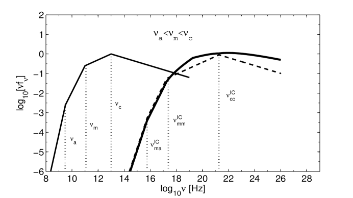
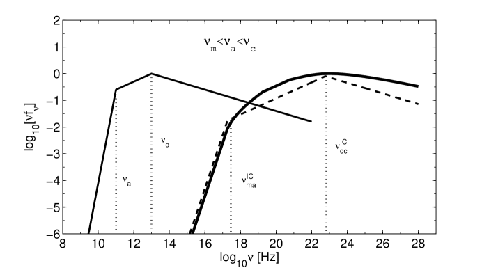
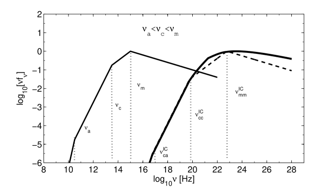
Figure 1: Total synchrotron $+$ SSC spectra for weak synchrotron reabsorption cases ($\nu_{\rm a}<\nu_{\rm c}$). The top panel is for $\nu_{\rm a}<\nu_{\rm m}<\nu_{\rm c}$ case; the middle panel is for $\nu_{\rm m}<\nu_{\rm a}<\nu_{\rm c}$ case; and the bottom panel is for $\nu_{\rm a}<\nu_{\rm c}<\nu_{\rm m}$ case. The thin solid line is synchrotron component. The thick solid line in the SSC component is drawn using the analytical approximations, while the dashed lines are the broken power-law approximation for comparison. In all the cases, the $\nu F_{\nu}$ peaks for both the synchrotron and the SSC components are normalized to unity.

We define ratio between the SSC luminosity and the synchrotron luminosity as the $X$ parameter similar to Sari & Esin (2001), i.e.,

$$X\equiv\frac{L_{\rm IC}}{L_{\rm syn}}=\frac{U_{\rm ph}}{U_{\rm B}},$$ (60)

where $U_{\rm ph}$ and $U_{\rm B}$ are the synchrotron photon energy density and magnetic field energy density, respectively.

For $\nu_{\rm a}<\nu_{\rm m}<\nu_{\rm c}$ (case I) and $\nu_{\rm m}<\nu_{\rm a}<\nu_{\rm c}$ (case II), the $\nu f_{\nu}$ peaks of the synchrotron and the SSC components are at $\nu_{\rm c}$ and $\nu_{\rm cc}^{IC}$, respectively (see Figure 1). One can estimate

$$X=\frac{L_{\rm IC}}{L_{\rm syn}} \sim \frac{\nu_{\rm cc}^{\rm{IC}}f_{\nu}^{\rm{IC}}(\nu_{\rm cc}^{\rm{IC}})}{\nu_{\rm c}f_{\nu}(\nu_{\rm c})}$$ (61)

$$\sim \frac{\nu_{\rm cc}^{\rm{IC}}R\sigma_{T}nf_{\rm{max}}x_{0}\left(\frac{\nu_{\rm cc}^{\rm{IC}}}{\nu_{\rm mm}^{\rm{IC}}}\right)^{\frac{1-p}{2}}}{\nu_{\rm c}f_{\rm{max}}\left(\frac{\nu_{\rm c}}{\nu_{\rm m}}\right)^{\frac{1-p}{2}}}$$

$$\sim 4x_{0}^{2}\sigma_{T}nR\gamma_{\rm c}^{2}\left(\frac{\gamma_{\rm c}}{\gamma_{\rm m}}\right)^{1-p},$$

which is consistent with Sari & Esin (2001). Note that when calculating $X$, we did not include the coefficients in the analytical approximations of the SSC component, which is of order unity.

For $\nu_{\rm a}<\nu_{\rm c}<\nu_{\rm m}$ (case III), the $\nu f_{\nu}$ peaks of the synchrotron and SSC components are at $\nu_{\rm m}$, and $\nu_{\rm mm}^{\rm IC}$, respectively. One therefore has

$$X=\frac{L_{\rm IC}}{L_{\rm syn}} \sim \frac{\nu_{\rm mm}^{\rm{IC}}f_{\nu}^{\rm{IC}}(\nu_{\rm mm}^{\rm{IC}})}{\nu_{\rm m}f_{\nu}(\nu_{\rm m})}$$ (62)

$$\sim \frac{\nu_{\rm mm}^{\rm{IC}}R\sigma_{T}nf_{\rm{max}}x_{0}\left(\frac{\nu_{\rm mm}^{\rm{IC}}}{\nu_{\rm cc}^{\rm{IC}}}\right)^{-\frac{1}{2}}}{\nu_{\rm m}f_{\rm{max}}\left(\frac{\nu_{\rm m}}{\nu_{\rm c}}\right)^{-\frac{1}{2}}}$$

$$\sim 4x_{0}^{2}\sigma_{T}nR\gamma_{\rm c}\gamma_{\rm m},$$

which is also consistent with Sari & Esin (2001).

3 Strong Synchrotron Self-Absorption Cases

When $\nu_{\rm a}>\nu_{\rm c}$, synchrotron/SSC cooling and self-absorption heating would reach a balance around a specific electron energy under certain conditions (see details in Appendix A). For such cases, the electron energy distribution and the photon spectrum are coupled, a numerical iterative procedure is needed to obtain the self-consistent solution. Ghisellini et al. (1988) solved the kinetic equation and found that the electron energy distribution would include two components: a thermal component shaped by synchrotron self-absorption heating, and a non-thermal power-law component. Based on their results (Ghisellini et al., 1988), the electron distribution is close but not strictly Maxwellian. Strictly, one needs to use equation (2) to calculate the SSC spectral component numerically. In the following, we make an approximation to derive analytical results. For the quasi-thermal component, we take $N(\gamma)\propto\gamma^{2}$ for $\gamma<\gamma_{\rm a}$ to denote the thermal component, and take a sharp cutoff at $\gamma_{\rm a}$. Above this energy, the electron energy distribution is taken as the standard (broken) power law distribution.

In particular, for $\nu_{\rm c}<\nu_{\rm a}<\nu_{\rm m}$, the electron distribution becomes

$$N(\gamma)=\left\{\begin{array}[]{ll}n\frac{3\gamma^{2}}{\gamma_{\rm a}^{3}},&\gamma\leq\gamma_{\rm a},\\ n\gamma_{\rm c}\gamma^{-2},&\gamma_{\rm a}<\gamma\leq\gamma_{\rm m}.\\ n\gamma_{\rm m}^{p-1}\gamma_{\rm c}\gamma^{-p-1},&\gamma>\gamma_{\rm m}.\end{array}\right.$$ (66)

For $\nu_{\rm m}<\nu_{\rm c}<\nu_{\rm a}$, one has

$$N(\gamma)=\left\{\begin{array}[]{ll}n\frac{3\gamma^{2}}{\gamma_{\rm a}^{3}},&\gamma\leq\gamma_{\rm a},\\ n(p-1)\gamma_{\rm m}^{p-1}\gamma_{\rm c}\gamma^{-p-1},&\gamma>\gamma_{\rm a}.\end{array}\right.$$ (69)

For $\nu_{\rm c}<\nu_{\rm m}<\nu_{\rm a}$, one has

$$N(\gamma)=\left\{\begin{array}[]{ll}n\frac{3\gamma^{2}}{\gamma_{\rm a}^{3}},&\gamma\leq\gamma_{\rm a},\\ n\gamma_{\rm m}^{p-1}\gamma_{\rm c}\gamma^{-p-1},&\gamma>\gamma_{\rm a}.\end{array}\right.$$ (72)

Following these new shapes of the electron distribution, the synchrotron photon spectra can be calculated, which also contain a thermal component and a (broken) power-law component. Still applying equation (2), one can analytically calculate the SSC spectral component for another three cases in this regime. We note that due to the simple approximation to the complicated electron pile-up process, the analytical results presented below are not as precise as those in the weak absorption cases.

3.1 Case IV: $\nu_{\rm c}<\nu_{\rm a}<\nu_{\rm m}$

In this case, the synchrotron photon spectrum reads

$$f_{\nu}=\left\{\begin{array}[]{ll}f_{\rm{max}}\left(\frac{\nu}{\nu_{\rm a}}\right)^{2},&\nu\leq\nu_{\rm a};\\ f_{\rm{max}}\mathfrak{R}\left(\frac{\nu}{\nu_{\rm a}}\right)^{-\frac{1}{2}},&\nu_{\rm a}<\nu\leq\nu_{\rm m};\\ f_{\rm{max}}\mathfrak{R}\left(\frac{\nu_{\rm m}}{\nu_{\rm a}}\right)^{-\frac{1}{2}}\left(\frac{\nu}{\nu_{\rm m}}\right)^{-\frac{p}{2}},&\nu>\nu_{\rm m};\end{array}\right.$$ (76)

where $\mathfrak{R}$ is the discontinuity ratio in the electron distribution at $\gamma_{\rm a}$,

$$\mathfrak{R}=\frac{\gamma_{\rm c}}{3\gamma_{\rm a}}~{}.$$ (77)

One can then derive

$$I=\left\{\begin{array}[]{ll}I_{1}\simeq f_{\rm{max}}x_{0}\left(\frac{1}{2}\mathfrak{R}+1\right)\left(\frac{\nu}{4\gamma^{2}\nu_{\rm a}x_{0}}\right),&\nu<4\gamma^{2}\nu_{\rm a}x_{0}\\ I_{2}\simeq\frac{1}{2}f_{\rm{max}}x_{0}\mathfrak{R}\left(\frac{\nu}{4\gamma^{2}\nu_{\rm a}x_{0}}\right)^{-\frac{1}{2}},&4\gamma^{2}\nu_{\rm a}x_{0}<\nu<4\gamma^{2}\nu_{\rm m}x_{0}\\ I_{3}\simeq\frac{3}{2(p+2)}f_{\rm{max}}x_{0}\mathfrak{R}\left(\frac{\nu_{\rm a}}{\nu_{\rm m}}\right)^{\frac{1}{2}}\left(\frac{\nu}{4\gamma^{2}\nu_{\rm m}x_{0}}\right)^{-\frac{p}{2}},&\nu>4\gamma^{2}\nu_{\rm m}x_{0}\\ \end{array}\right.$$ (81)

and

$$f_{\nu}^{\rm{IC}} \simeq R\sigma_{\rm T}nf_{\rm{max}}x_{0}$$ (82)

$$\times \left\{\begin{array}[]{ll}\left(\frac{1}{2}\mathfrak{R}+1\right)\left(\mathfrak{R}+4\right)\left(\frac{\nu}{\nu_{\rm aa}^{\rm{IC}}}\right),&\nu<\nu_{\rm aa}^{\rm{IC}};\\ \mathfrak{R}\left(\frac{\nu}{\nu_{\rm aa}^{\rm{IC}}}\right)^{-\frac{1}{2}}\left[\frac{1}{6}\mathfrak{R}+\frac{9}{10}+\frac{1}{4}\mathfrak{R}\ln{\left(\frac{\nu}{\nu_{\rm aa}^{\rm{IC}}}\right)}\right],&\nu_{\rm aa}^{\rm{IC}}<\nu<\nu_{\rm am}^{\rm{IC}};\\ \mathfrak{R}^{2}\left(\frac{\nu}{\nu_{\rm aa}^{\rm{IC}}}\right)^{-\frac{1}{2}}\left[\frac{3}{p-1}-\frac{1}{2}+\frac{3}{4}\ln{\left(\frac{\nu_{\rm mm}^{\rm IC}}{\nu}\right)}\right],&\nu_{\rm am}^{\rm{IC}}<\nu<\nu_{\rm mm}^{\rm{IC}};\\ \frac{9}{2(p+2)}\mathfrak{R}^{2}\left(\frac{\nu_{\rm a}}{\nu_{\rm m}}\right)\left(\frac{\nu}{\nu_{\rm mm}^{\rm{IC}}}\right)^{-\frac{p}{2}}\left[\frac{4}{p+3}\left(\frac{\gamma_{\rm a}}{\gamma_{\rm m}}\right)^{p-1}\frac{\gamma_{\rm a}}{\gamma_{\rm c}}+\frac{3(p+1)}{(p-1)(p+2)}+\frac{1}{2}\ln{\frac{\nu}{\nu_{\rm mm}^{\rm IC}}}\right],&\nu>\nu_{\rm mm}^{\rm{IC}}.\end{array}\right.$$ (87)

In this case, there are two peaks in the $\nu F_{\nu}$ spectrum for the synchrotron and SSC components, respectively. For the synchrotron component, the thermal peak is at $(25/9)\nu_{\rm a}\simeq 2.8\nu_{a}$, and the non-thermal peak is at $\nu_{\rm m}$. For the SSC component, the thermal peak at $\nu_{\rm aa}^{IC}$, and the non-thermal peak at $\nu_{\rm mm}^{\rm IC}$. The relative importance of the two peaks depend on the relative location of $\nu_{\rm a}$ with respect to $\nu_{\rm c}$ and $\nu_{\rm m}$. More specifically, the spectrum is non-thermal-dominated when $\nu_{\rm a}<\sqrt{\nu_{\rm m}\nu_{\rm c}}$, and is thermal-dominated when $\nu_{\rm a}>\sqrt{\nu_{\rm m}\nu_{\rm c}}$.

In Figure 2, we compare the above simplified analytical approximation (solid) with a simplest power law prescription (dashed) of the SSC component. The non-thermal-dominated and the thermal-dominated cases are presented in Figures 2a and 2b, respectively. Below $\nu_{\rm mm}^{\rm IC}$, similar to the weak self-absorption regime (cases I-III), the logarithmic terms make the analytical spectrum harder than the simple broken power-law approximation above the non-thermal $\nu F_{\nu}$ peak frequency. At high frequencies, the simple broken power-law approximation is not adequate to represent the true SSC spectrum.

3.2 Case V and VI: $\nu_{\rm a}>{\rm max}(\nu_{\rm m},\nu_{\rm c})$

For these two cases ($\nu_{\rm m}<\nu_{\rm c}<\nu_{\rm a}$ and $\nu_{\rm c}<\nu_{\rm m}<\nu_{\rm a}$), the treatments and results are rather similar to each other. we take $\nu_{\rm m}<\nu_{\rm c}<\nu_{\rm a}$ as an example. In this case, the synchrotron spectrum reads

$$f_{\nu}=\left\{\begin{array}[]{ll}f_{\rm{max}}\left(\frac{\nu}{\nu_{\rm a}}\right)^{2},&\nu\leq\nu_{\rm a};\\ f_{\rm{max}}\mathfrak{R}\left(\frac{\nu}{\nu_{\rm a}}\right)^{-\frac{p}{2}},&\nu>\nu_{\rm a};\\ \end{array}\right.$$ (90)

where

$$\mathfrak{R}=(p-1)\frac{\gamma_{\rm c}}{3\gamma_{\rm a}}\left(\frac{\gamma_{\rm m}}{\gamma_{\rm a}}\right)^{p-1}.$$ (91)

Applying equation (2), the inner integral $I$ can be then approximated as

$$I=\left\{\begin{array}[]{ll}I_{1}\simeq f_{\rm{max}}x_{0}\left(\frac{3\mathfrak{R}}{2(p+2)}+1\right)\left(\frac{\nu}{4\gamma^{2}\nu_{\rm a}x_{0}}\right),&\nu<4\gamma^{2}\nu_{\rm a}x_{0}\\ I_{2}\simeq\frac{3}{2(p+2)}f_{\rm{max}}x_{0}\mathfrak{R}\left(\frac{\nu}{4\gamma^{2}\nu_{\rm a}x_{0}}\right)^{-\frac{p}{2}},&\nu>4\gamma^{2}\nu_{\rm a}x_{0}.\end{array}\right.$$ (94)

Integrating over the outer integral, one gets

$$f_{\nu}^{\rm{IC}} \simeq R\sigma_{\rm T}nf_{\rm{max}}x_{0}$$ (95)

$$\times \left\{\begin{array}[]{ll}\left(\frac{\mathfrak{3R}}{2(p+2)}+1\right)\left(\frac{\mathfrak{3R}}{p+2}+4\right)\left(\frac{\nu}{\nu_{\rm aa}^{\rm{IC}}}\right),&\nu<\nu_{\rm aa}^{\rm{IC}};\\ \frac{1}{p+2}\left[\frac{6\mathfrak{R}}{p+3}+\mathfrak{R}\left(\frac{9\mathfrak{R}}{2(p+2)}+1\right)+\frac{9\mathfrak{R}^{2}}{4}\ln{\left(\frac{\nu}{\nu_{\rm aa}^{\rm{IC}}}\right)}\right]\left(\frac{\nu}{\nu_{\rm aa}^{\rm{IC}}}\right)^{-\frac{p}{2}},&\nu>\nu_{\rm aa}^{\rm{IC}};\\ \end{array}\right.$$ (98)

The case of $\nu_{\rm c}<\nu_{\rm m}<\nu_{\rm a}$ is almost identical to the above $\nu_{\rm m}<\nu_{\rm c}<\nu_{\rm a}$. The only difference is that the expression of $\mathfrak{R}$ is modified to

$$\mathfrak{R}=\frac{\gamma_{\rm c}}{3\gamma_{\rm a}}\left(\frac{\gamma_{\rm m}}{\gamma_{\rm a}}\right)^{p-1}.$$ (99)

This is reasonable, since in the fast cooling case, the electron energy spectral index is $p=2$, so that the factor $(p-1)$ can be reduced to 1. The analytical results and simple broken power-law approximation in this regime is identical to Figure 3c. We note again that full numerical calculations are needed to obtain more accurate results.

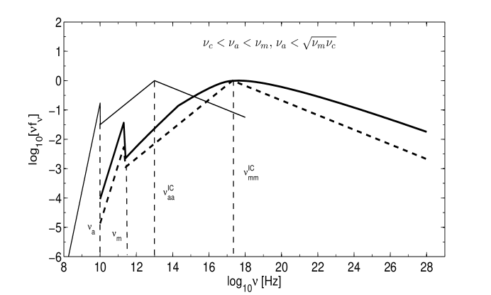
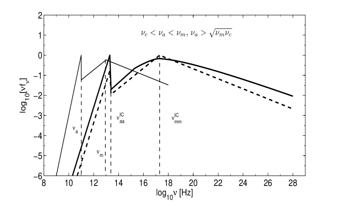
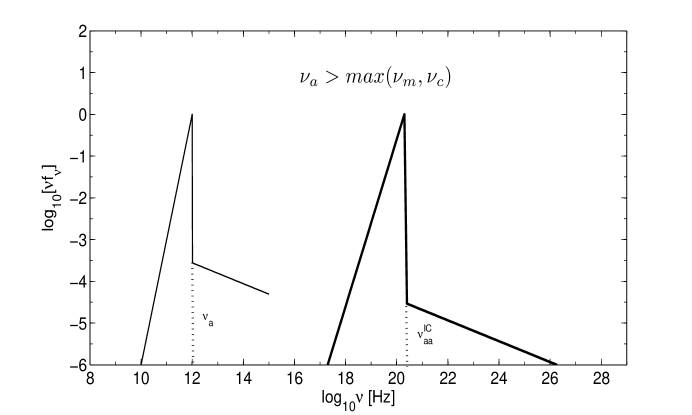
Figure 2: Same as Figure 1, but for strong synchrotron reabsorption cases . The top panel is for $\nu_{\rm c}<\nu_{\rm a}<\nu_{\rm m}$ and $\nu_{\rm a}<\sqrt{\nu_{\rm m}\nu_{\rm c}}$ case; the middle panel is for $\nu_{\rm c}<\nu_{\rm a}<\nu_{\rm m}$ and $\nu_{\rm a}>\sqrt{\nu_{\rm m}\nu_{\rm c}}$ case; and the bottom panel is for $\nu_{\rm a}>{\rm max}(\nu_{\rm m},\nu_{\rm c})$ case. All the solid lines are analytical approximations and the dashed lines are broken power-law approximations.

Finally, we investigate the $X$ parameter in the strong synchrotron self-absorption regime.

For $\nu_{\rm c}<\nu_{\rm a}<\nu_{\rm m}$ (case IV), if the spectrum is non-thermal-dominated, the synchrotron and SSC emission components peak at $\nu_{\rm m}$ and $\nu_{\rm mm}^{\rm IC}$, respectively. One thus has

$$X=\frac{L_{\rm IC}}{L_{\rm syn}} \sim \frac{\nu_{\rm mm}^{\rm{IC}}f_{\nu}^{\rm{IC}}(\nu_{\rm mm}^{\rm{IC}})}{\nu_{\rm m}f_{\nu}(\nu_{\rm m})}$$ (100)

$$\sim \frac{\nu_{\rm mm}^{\rm{IC}}R\sigma_{\rm T}nf_{\rm{max}}x_{0}\mathfrak{R}^{2}\left(\frac{\nu_{\rm mm}^{\rm{IC}}}{\nu_{\rm aa}^{\rm{IC}}}\right)^{-\frac{1}{2}}}{\nu_{\rm m}\mathfrak{R}f_{\rm{max}}\left(\frac{\nu_{m}}{\nu_{a}}\right)^{-\frac{1}{2}}}$$

$$\sim 4x_{0}^{2}\sigma_{\rm T}nR\gamma_{\rm c}\gamma_{\rm m}.$$

If the spectrum is thermal-dominated, the synchrotron and SSC emission components peak at $\nu_{\rm a}$ and $\nu_{\rm aa}^{\rm IC}$, respectively. One has

$$X=\frac{L_{\rm IC}}{L_{\rm syn}} \sim \frac{\nu_{\rm aa}^{\rm{IC}}f_{\nu}^{\rm{IC}}(\nu_{\rm aa}^{\rm{IC}})}{\nu_{\rm a}f_{\nu}(\nu_{\rm a})}$$ (101)

$$\sim \frac{\nu_{\rm aa}^{\rm{IC}}R\sigma_{\rm T}nf_{\rm{max}}x_{0}}{\nu_{\rm a}f_{\rm{max}}}$$

$$\sim 4x_{0}^{2}\sigma_{\rm T}nR\gamma_{\rm a}^{2}.$$

In general, the $X$ parameter for $\nu_{\rm c}<\nu_{\rm a}<\nu_{\rm m}$ (case IV) is $4x_{0}^{2}\sigma_{\rm T}nR\cdot{\rm max}(\gamma_{\rm a}^{2},\gamma_{\rm c}\gamma_{\rm m})$.

For $\nu_{\rm m}<\nu_{\rm c}<\nu_{\rm a}$ (case V) and $\nu_{\rm c}<\nu_{\rm m}<\nu_{\rm a}$ (case VI), the synchrotron and SSC emission components peak at $\nu_{\rm a}$ and $\nu_{\rm aa}^{IC}$, respectively. In this case, one has

$$X=\frac{L_{\rm IC}}{L_{\rm syn}} \sim \frac{\nu_{\rm aa}^{\rm{IC}}f_{\nu}^{\rm{IC}}(\nu_{\rm aa}^{\rm{IC}})}{\nu_{\rm a}f_{\nu}(\nu_{\rm a})}$$ (102)

$$\sim \frac{\nu_{\rm aa}^{\rm{IC}}R\sigma_{\rm T}nf_{\rm{max}}x_{0}}{\nu_{\rm a}f_{\rm{max}}}$$

$$\sim 4x_{0}^{2}\sigma_{\rm T}nR\gamma_{\rm a}^{2}.$$

which is same as the thermal-dominated case for $\nu_{\rm c}<\nu_{\rm a}<\nu_{\rm m}$ (case IV). So in general the expression of $X$ is equation (102) only if the spectrum is thermal-dominated.

4 Conclusion and discussion

We have extended the analysis of Sari & Esin (2001) and derived the analytical approximations of the SSC spectra of all possible orders of the three synchrotron characteristic frequencies $\nu_{\rm a}$, $\nu_{\rm m}$, and $\nu_{\rm c}$. Based on the relative order between $\nu_{\rm a}$ and $\nu_{\rm c}$, we divide the six possible orders into two regimes.

In the weak self-absorption regime $\nu_{\rm a}<\nu_{\rm c}$, self-absorption does not affect the electron energy distribution. Two cases in this regime have been studied by Sari & Esin (2001). Our results are consistent with theirs (except the two typos in their paper). For the other regime $\nu_{\rm m}<\nu_{\rm a}<\nu_{\rm c}$, we find that the SSC spectrum is linear to $\nu$ all the way to $\nu_{\rm ma}^{\rm{IC}}$, and there is no break corresponding to $\nu_{\rm mm}^{\rm{IC}}$.

In the strong self-absorption $\nu_{\rm a}>\nu_{\rm c}$ regime, synchrotron self-absorption heating balances synchrotron/SSC cooling, leading to pile-up of electrons at a certain energy, so that the electron energy distribution is significantly altered, with an additional thermal component besides the non-thermal power law component. Both the synchrotron and the SSC spectral components become two-hump shaped. To get an analytical approximation of the SSC spectrum, we simplified the quasi-thermal electron energy distribution as a power law with a sharp cutoff above the piling up energy, and derived the analytical approximation results of the synchrotron and SSC spectral components. We suggest that for the thermal-dominated cases, i.e. $\nu_{\rm a}>\sqrt{\nu_{\rm m}\nu_{\rm c}}$ in the $\nu_{\rm c}<\nu_{\rm a}<\nu_{\rm m}$ regime or the $\nu_{\rm a}>\max(\nu_{\rm m},\nu_{\rm c})$ regime, full numerical calculations are needed to get accurate results.

In general, the SSC component roughly tracks the shape of the seed synchrotron component, but is smoother and harder at high energies. For all the cases, we compare our analytical approximation results of SSC component with the simplest broken power-law prescription. We find that in general the presence of the logarithmic terms in the high energy range makes the SSC spectrum harder than the broken power-law approximation. One should consider these terms when studying high energy emission. The only exceptions are the $\nu_{\rm a}>\max(\nu_{\rm m},\nu_{\rm c})$ regimes. However, in these regimes the analytical approximations may be no longer good, and one should appeal to full numerical calculations.

Our newly derived spectral regimes may find applications in astrophysical objects with high “compactness” (i.e. high luminosity, and small size). In these cases, $\nu_{\rm a}$ can be higher than $\nu_{\rm c}$ or $\nu_{\rm m}$, or even both (see Appendix A for the critical condition). For example, in the early afterglow phase of GRBs, slow cooling may be relevant, and the radio afterglow is self-absorbed with $\nu_{\rm a}$ above $\nu_{\rm m}$ (e.g. Chandra & Frail, 2012). In the prompt emission phase when fast cooling is more relevant, the self-absorption frequency can be above $\nu_{\rm c}$ (e.g. Shen & Zhang, 2009).

An example of the extreme case $\nu_{\rm a}>{\rm max}(\nu_{\rm m},\nu_{\rm c})$ can be identified for a GRB problem. For a dense circumburst medium with a wind-like ($n\propto r^{-2}$) structure, in the reverse shock region, the condition $\nu_{\rm a}>\max(\nu_{\rm m},\nu_{\rm c})$ can be satisfied (e.g. Kobayashi et al., 2004). For a GRB with isotropic energy $E=10^{52}E_{52}$, initial Lorentz factor $\Gamma_{0}=100\Gamma_{0,2}$, initial shell width $\Delta=10^{12}\Delta_{12}$ running into stellar wind with density $\rho=(5\times 10^{11}{\rm g~{}cm^{-1}})A_{*}r^{-2}$, one can derive following parameters at the shock crossing radius $r_{\times}$: The blastwave Lorentz factor $\Gamma_{\times}=25.8A_{*}^{-1/4}\Delta_{12}^{-1/4}E_{52}^{1/4}$, $\nu_{\rm m}=3.1\times 10^{14}~{}{\rm Hz}~{}[g(p)/g(2.3)]A_{*}\Delta_{12}^{-1/2}E_{52}^{-1/2}\epsilon_{e,-1}^{2}\epsilon_{B,-2}^{1/2}\Gamma_{0,2}^{2}$, $\nu_{c}=1.2\times 10^{12}~{}{\rm Hz}~{}A_{*}^{-2}\Delta_{12}^{1/2}E_{52}^{1/2}\epsilon_{B,-2}^{-3/2}$, $\nu_{a}=4.6\times 10^{14}~{}{\rm Hz}~{}A_{*}^{3/5}\Delta_{12}^{-11/10}E_{52}^{1/10}\epsilon_{B.-2}^{3/10}\Gamma_{0,2}^{-2/5}$. Here $\epsilon_{e}=0.1\epsilon_{e,-1}$ and $\epsilon_{B}=0.01\epsilon_{B,-2}$ are microphysics shock parameters for the internal energy fraction that goes to electrons and magnetic fields, $p$ is the electron spectral index, and $g(p)=(p-2)/(p-1)$. We can see that for typical parameters, $\nu_{a}>{\rm max}(\nu_{c},\nu_{m})$ is satisfied. In this regime, one should check whether the “Razin” plasma effect is important. At shock crossing time, the comoving number density of the shocked ejecta region is $n^{\prime}=2.3\times 10^{8}~{}{\rm cm^{-3}}~{}A_{*}^{5/4}\Delta_{12}^{-7/4}E_{52}^{-1/4}\Gamma_{0,1}^{-1}$. Noticing that the comoving plasma angular frequency is $\omega^{\prime}_{p}=5.63\times 10^{4}~{}{\rm s^{-1}}{n^{\prime}}^{1/2}$, one can write the plasma frequency in the observer frame as $\nu_{p}=1.4\times 10^{11}~{}{\rm Hz}~{}A_{*}^{3/8}\Delta_{12}^{-9/8}E_{52}^{1/8}\Gamma_{0,2}^{-1/2}$. Multiplying by $\gamma_{\rm a}=102A_{*}^{1/20}\Delta_{12}^{-1/20}E_{52}^{1/20}\epsilon_{B.-2}^{-1/10}\Gamma_{0,2}^{-1/5}$, one gets $\gamma_{\rm a}\nu_{p}=1.4\times 10^{13}~{}{\rm Hz}~{}A_{*}^{17/40}\Delta_{12}^{-47/40}E_{52}^{7/40}\epsilon_{B,-2}^{-1/10}\Gamma_{0,2}^{-7/10}$, which is much smaller than $\nu_{\rm a}$. This suggests that the Razin effect is not important (Rybicki & Lightman, 1979), and the dominant mechanism to suppress synchrotron emission at low energies is synchrotron self-absorption. Notice that for this particular problem, the second order Comptonization may not be suppressed by the Klein-Nishina effect, and one has to introduce it for a fully self-consistent treatment.

Appendix A Condition of electron pile-up and strong absorption

By applying the Einstein coefficients and their relations to a system with three energy levels, Ghisellini et al. (1991) have derived one useful analytical expression of the cross section for synchrotron self-absorption:

$$\sigma_{\rm S}(\gamma,\nu)=\left\{\begin{array}[]{ll}\frac{2^{2/3}\sqrt{3}\pi\Gamma^{2}(4/3)}{5}\frac{\sigma_{\rm T}}{\alpha_{\rm f}}\frac{B_{\rm cr}}{B}\left(\frac{\gamma\nu}{3\nu_{\rm L}}\right)^{-5/3},&\frac{\nu_{\rm L}}{\gamma}<\nu\ll\frac{3}{2}\gamma^{2}\nu_{\rm L},\\ \frac{\sqrt{3}}{2}\pi^{2}\frac{\sigma_{\rm T}}{\alpha_{\rm f}}\frac{B_{\rm cr}}{B}\frac{1}{\gamma^{3}}\left(\frac{\nu_{\rm L}}{\nu}\right)\rm{exp}\left(\frac{-2\nu}{3\gamma^{2}\nu_{\rm L}}\right),&\nu\gg\frac{3}{2}\gamma^{2}\nu_{\rm L}.\end{array}\right.$$ (105)

where $\gamma$ is the relevant electron Lorentz factor, $\nu$ is photon frequency being absorbed, $\alpha_{\rm f}$ is the fine structure constant, $B_{\rm cr}=\alpha_{\rm f}(m_{e}c^{2}/r_{e}^{3})^{1/2}\approx 4.4\times 10^{13}\rm G$ is the critical magnetic field strength, $r_{e}$ is the classical electron radius, and $\nu_{\rm L}=eB/2\pi m_{e}c$ is the electron cyclotron frequency. All the parameters introduced in this section are in the comoving frame.

For a simple derivation of the electron pile-up condition, we take an approximate form

$$\sigma_{\rm S}(\gamma,\nu)=\left\{\begin{array}[]{ll}\frac{2^{2/3}\sqrt{3}\pi\Gamma^{2}(4/3)}{5}\frac{\sigma_{\rm T}}{\alpha_{\rm f}}\frac{B_{\rm cr}}{B}\left(\frac{\gamma\nu}{3\nu_{\rm L}}\right)^{-5/3},&\frac{\nu_{\rm L}}{\gamma}<\nu\leq\frac{3}{2}\gamma^{2}\nu_{\rm L},\\ 0,&\nu>\frac{3}{2}\gamma^{2}\nu_{\rm L}.\end{array}\right.$$ (108)

For electrons with Lorenz factor $\gamma$, the heating rate due to synchrotron self-absorption can be estimated as

$$\dot{\gamma}^{+}(\gamma)=\int_{0}^{\infty}c\cdot n_{\nu}\cdot h\nu\cdot\sigma_{\rm S}(\gamma,\nu)\cdot d\nu$$ (109)

where $n_{\nu}$ is the specific photon number density at frequency $\nu$ contributed by all the electrons.

The cooling rate for electrons with Lorentz factor of $\gamma$ is

$$\dot{\gamma}^{-}(\gamma) = (1+Y)\cdot P_{\rm syn}$$ (110)

$$= (1+Y)\times\frac{4}{3}\sigma_{\rm T}c\gamma^{2}\frac{B^{2}}{8\pi},$$

where $Y\equiv\frac{P_{\rm ssc}}{P_{\rm syn}}$ is the Compton parameter.

By balancing the heating and cooing rate, one can easily obtain the critical electron Lorentz factor $\gamma_{\rm cr}$, which satisfies

$$\dot{\gamma}^{+}(\gamma_{\rm cr})=\dot{\gamma}^{-}(\gamma_{\rm cr})$$ (111)

Initially, the photon spectrum has not been revised through self-absorption, i.e., $n_{\nu}\propto\nu^{1/3}$. One therefore has

$$\gamma_{\rm cr}=2.1\times 10^{4}B^{-3/5}{\cal F}_{\rm\nu,max}^{3/10}\gamma_{c}^{-1/5}(1+Y)^{-3/10}$$ (112)

The electron pile-up (strong absorption) condition can be expressed as

$$\gamma_{\rm cr}>\gamma_{c}=\frac{6\pi m_{e}c}{\sigma_{\rm T}B^{2}t(1+Y)}~{}.$$ (113)

With equations 108 - 113, the pile-up condition can be expressed as

$$\left(\frac{B}{100\rm G}\right)^{2}\times\left(\frac{t}{100\rm s}\right)^{4/3}\times{\cal F}_{\rm\nu,max}^{1/3}\times\left(\frac{1+Y}{2}\right)>1$$ (114)

where

$${\cal F}_{\rm\nu,max}=\frac{f_{\rm max}}{\Gamma(1+z)}\left(\frac{d_{\rm L}}{R}\right)^{2}=1~{}{\rm erg~{}cm^{-2}~{}s^{-1}~{}Hz^{-1}}~{}\frac{f_{\rm max,mJy}}{\Gamma_{2}(1+z)}\left(\frac{d_{\rm L,28}}{R_{14}}\right)^{2}$$ (115)

is the synchrotron peak flux in the emission region. Here $d_{\rm L}$ is the luminosity distance of the source, and $R$ is the distance of the emission region from the central engine.

One can immediately see that this condition is very difficult to satisfy. It requires a strong magnetic field, long dynamical time scale and high synchrotron flux. In the GRB afterglow problem, for forward shock emission, $B$ decreases with $t$ rapidly, and there is essentially no parameter space to satisfy the condition. This condition may be realized in extreme conditions, e.g. the reverse shock emission during shock crossing phase for a wind medium, as discussed in Sect.4 in the main text.

One interesting note is that SSC cooling only enhances the pile-up condition. Once the pile-up condition is satisfied for synchrotron cooling only, adding SSC cooling only makes the condition more easily satisfied (as shown in equation 114).

Once the electron pile-up process is triggered, both electron distribution and photon spectrum would be modified, so that the value of $\gamma_{\rm cr}$ is modified correspondingly. According to the numerical calculation results (Ghisellini et al., 1988, 1991, 1998a), the electron distribution is dominated by a quasi-thermal component until a “transition” Lorentz factor $\gamma_{\rm t}$, above which the electrons go back to the optically-thin normal power law. In this case, $\gamma_{\rm cr}$ should be around the thermal peak, and $\gamma_{a}$ should be around the “transition” Lorentz factor $\gamma_{\rm t}$, which is slightly larger than $\gamma_{\rm cr}$. Consequently, one would roughly have $\gamma_{a}\sim\gamma_{\rm cr}\sim\gamma_{t}$, so that the assumption of a sharp cutoff in the electron distribution around this energy is justified. In the main text, we did not differentiate the three Lorentz factors, and only adopt $\gamma_{a}$ in the expressions.

References

• Blumenthal & Gould ( 1970) Blumenthal, G. R., & Gould, R. J. 1970, Rev. Mod. Phys., 42, 237
• Chandra & Frail (2012) Chandra, P., & Frail, D., 2012, ApJ, 746, 156
• Chiang & Böttcher (2002) Chiang, J. & Böttcher, M. 2002, ApJ, 564, 92
• Dermer et al. (2000) Dermer, C. D., BÓttcher, M., Chiang, J. 2000, ApJ, 537, 255
• Ghisellini et al. (1988) Ghisellini, G., Guilbert, P., Svensson, R., 1988, ApJL, 334, 5
• Ghisellini et al. (1991) Ghisellini, G., Svensson, R., 1991, MNRAS, 252, 313
• Ghisellini et al. (1998a) Ghisellini, G., Haardt, F., Svensson, R., 1998, MNRAS, 297, 348
• Ghisellini et al. (1998b) Ghisellini, G., Celotti, A., Fossati, G., Maraschi, L., Comastri, A. 1998, MNRAS, 301, 451
• Gou et al. (2007) Gou, L.-J., Fox, D.B., Mészáros, P. 2007, ApJ, 668, 1083
• Kobayashi et al. (2004) Kobayashi, S., Mészáros, P., Zhang, B., 2004, ApJL, 601, 13
• Kobayashi et al. (2007) Kobayashi, S., Zhang, B., Mészáros, P., Burrows, D. 2007, ApJ, 655, 391
• Mészáros et al. (1994) Mészáros, P., Rees, M. J., & Papathanassiou, H., 1994, ApJ, 432, 181
• Nakar et al. (2009) Nakar, E., Ando, S., & Sari, R., 2009, ApJ, 703, 675
• Panaitescu & Kumar (2000) Panaitescu, A. & Kumar, P. 2000, ApJ, 543, 66
• Piran et al. (2009) Piran, T., Sari, R., Zou, Y.-C. 2009, MNRAS, 393, 1107
• Rees (1967) Rees, M. J. 1967, MNRAS, 137, 429
• Rybicki & Lightman (1979) Rybicki, G. B., & Lightman, A. P. 1979, Radiative Processes in Astrophysics (New York: John Wiley & Sons)
• Sari et al. (1998) Sari, R., Piran, T, & Narayan R. 1998, ApJL, 497, 17
• Sari & Esin (2001) Sari, R., & Esin, A., 2001, ApJ, 548, 787
• Shen & Zhang (2009) Shen, R.-F., & Zhang, B. 2009, MNRAS, 398, 1936
• Uhm & Zhang (2013) Uhm, Z. L. & Zhang, B. 2013, arXiv:1303.2704
• Wang et al. (2001) Wang, X. Y., Dai, Z. G., & Lu, T. 2001, ApJ, 556, 1010
• Wei & Lu (1998) Wei, D. M., & Lu, T. 1998, ApJ, 505, 252
• Wu et al. (2004) Wu, X. F., Dai, Z. G., Huang, Y. F., & Ma, H. T., 2004, RAA, 4, 455
• Zhang & Mészáros (2001) Zhang, B., & Mészáros, P. 2001, ApJ, 559, 110
• Zhang et al. (2012) Zhang, J., Liang, E.-W., Zhang, S.-N., Bai, J.-M. 2012, ApJ, 752,157
• Zou et al. (2009) Zou, Y.-C, Fan, Y.-Z., & Piran, T. 2009, MNRAS, 396, 1163