Dirac tachyons and antitachyons in many-particle system

Abstract

A consistent description of charged many-tachyon Fermi system is developed. Tachyons and antitachyons have the same chemical potential $\mu_{+}=\mu_{-}$ because the axial coupling constant $g_{+}=g_{-}$ is invariant under the charge conjugation, in contrast to reversion of the electric charge $e_{+}=-e_{-}$. The axial density $n_{5}=\left\langle\bar{\psi}\gamma^{0}\gamma_{5}\psi\right\rangle$ is incorporated in the thermodynamical functions instead of $\left\langle\bar{\psi}\gamma^{0}\psi\right\rangle$ which is not associated with any conserved quantity. The number of tachyons and antitachyons are undefined but it is possible to estimate their difference and establish a link between the total electric charge density $en$ and $n_{5}$.

1 Introduction

Tachyon is a substance that moves faster than light. Its energy spectrum satisfies dispersion relation

$$\varepsilon_{p}^{2}=p^{2}-m^{2}$$ (1)

and its group velocity

$$v=\frac{d\varepsilon_{p}}{dp}=\frac{p}{\sqrt{p^{2}-m^{2}}}$$ (2)

exceeds the speed of light in vacuum $c=1$, relative to any reference frame.

Tachyons are commonly known in the field theory [1] and nonlinear optics [2]. The Lagrangian of a free fermionic tachyon [3, 4]$L_{0}=\bar{\psi}\left(i\gamma_{5}\gamma^{\mu}\partial_{\mu}-m\right)\psi$ corresponds to the equation of motion

$$\left(i\gamma^{\mu}\partial_{\mu}-\gamma_{5}m\right)\psi=0$$ (3)

whose plane wave solution

$$\psi=\left(\begin{array}[]{c}\phi\\ \chi\end{array}\right)\exp\left(i\vec{p}\cdot\vec{r}-i\varepsilon_{p\,}t\right)$$ (4)

results in the single-particle energy spectrum (1). The motion of tachyon in the presence of electromagnetic field $A_{\mu}$ is described by equation [5]

$$\left(i\gamma^{\mu}\left(\partial_{\mu}+ieA_{\mu}\right)-\gamma_{5}m\right)\psi=0$$ (5)

that corresponds to appearance of interaction term $-e\bar{\psi}\gamma_{5}\gamma^{\mu}A_{\mu}\psi$ in the free tachyonic Lagrangian. The equation of motion

$$\left(\gamma^{\mu}\left(i\partial_{\mu}-eA_{\mu}\right)-\gamma_{5}m-g\gamma_{5}\gamma^{\mu}\omega_{\mu}\right)\psi=0$$ (6)

is written when the relevant Lagrangian $L=L_{0}-e\bar{\psi}\gamma_{5}\gamma^{\mu}A_{\mu}\psi-g\bar{\psi}\gamma^{\mu}\omega_{\mu}\psi$ includes the coupling term associated with vector field $\omega_{\mu}$.

When we consider an ensemble of particle and antiparticles in finite volume $V=\int d^{3}r$, we use standard definitions of the particle number density

$$n\equiv\left\langle\bar{\psi}\gamma^{0}\psi\right\rangle=\frac{\gamma}{\left(2\pi\right)^{3}}\int\bar{\psi}\gamma^{0}\psi\,d^{3}p$$ (7)

and axial density

$$n_{5}\equiv\left\langle\bar{\psi}\gamma^{0}\gamma_{5}\psi\right\rangle=\frac{\gamma}{\left(2\pi\right)^{3}}\int\bar{\psi}\gamma^{0}\gamma_{5}\psi\,d^{3}p$$ (8)

The relevant total charges

$$\left\langle Q_{e}\right\rangle\equiv\left(e_{+}n_{+}+e_{-}n_{-}\right)V$$ (9)

$$\left\langle Q_{g}\right\rangle\equiv\left(g_{+}n_{5+}+g_{-}n_{5-}\right)V$$ (10)

include contributions from the two species that depend on the sign of elementary charges of particles $e_{+}$, $g_{+}$ and antiparticles $e_{-}$, $g_{-}$.

The electric charge conjugation [5] $e_{+}=-e_{-}\equiv e$ implies that the total electric charge of tachyons and antitachyons

$$Q_{e}\equiv e\left(n_{+}-n_{-}\right)V$$ (11)

coincides with the relevant expression for ordinary fermions and antifermions [6]. Most natural assumption $g_{-}=-g_{+}$ would lead to formula similar to (11) but relation between $g_{+}$ and $g_{-}$ is not evident beforehand. It is necessary to check the charge conjugation of tachyonic Dirac equation (6) and establish what consequences it implies to the thermodynamics of a many-tachyon system.

2 Charge conjugation

Equation (6) is equivalent to

$$\left(\gamma_{5}\gamma^{\mu}\left(i\partial_{\mu}-eA_{\mu}\right)-m-g\gamma^{\mu}\omega_{\mu}\right)\psi=0$$ (12)

The difference between $e$ and $g$ is evident from the corresponding bilinear transforms. Let us demonstrate it directly, following the previous analysis [5] and considering the charge conjugation of equation (6) or (12). The action of Hermite operator $\dagger$ (transposition and complex conjugation) results in

$$\psi^{\dagger}\left(-i\left[\gamma_{5}\gamma^{\mu}\right]^{\dagger}\partial_{\mu}-e\left[\gamma_{5}\gamma^{\mu}\right]^{\dagger}A_{\mu}-m-g\gamma^{\mu\dagger}\omega_{\mu}\right)=0$$ (13)

Presenting $\psi^{\dagger}\equiv\psi^{\dagger}\gamma^{0}\gamma^{0}=\bar{\psi}\gamma^{0}$ and multiplying equation (13) by $\gamma^{0}$ from the right, we have

$$\bar{\psi}\gamma^{0}\left(-i\left[\gamma_{5}\gamma^{\mu}\right]^{\dagger}\partial_{\mu}-e\left[\gamma_{5}\gamma^{\mu}\right]^{\dagger}A_{\mu}-m-g\gamma^{\mu\dagger}\omega_{\mu}\right)\times\gamma^{0}=0$$ (14)

Using identities

$$\gamma^{0}\gamma^{\mu\dagger}\gamma^{0}=\gamma^{\mu}\qquad\gamma^{\mu}\gamma_{5}=-\gamma_{5}\gamma^{\mu}\qquad\gamma_{5}=\gamma_{5}^{\dagger}\qquad\gamma^{0}\gamma_{5}\gamma^{0}=-\gamma_{5}$$ (15)

and

$$\gamma^{0}\left[\gamma_{5}\gamma^{\mu}\right]^{\dagger}\gamma^{0}=\gamma^{0}\gamma^{\mu\dagger}\gamma_{5}^{\dagger}\gamma^{0}=\gamma^{0}\gamma^{\mu\dagger}\gamma^{0}\gamma^{0}\gamma_{5}\gamma^{0}=\gamma_{5}\gamma^{\mu}$$ (16)

we obtain

$$\bar{\psi}\left(-i\gamma_{5}\gamma^{\mu}\partial_{\mu}-e\gamma_{5}\gamma^{\mu}A_{\mu}-m-g\gamma^{\mu}\omega_{\mu}\right)\gamma^{0}=0$$ (17)

Transposition of (17) yields

$$\left(i\left[\gamma_{5}\gamma^{\mu}\right]^{T}\partial_{\mu}+e\left[\gamma_{5}\gamma^{\mu}\right]^{T}A_{\mu}+m+g\gamma^{\mu T}\omega_{\mu}\right)\bar{\psi}^{T}=0$$ (18)

that can be also written in the equivalent form

$$\left(i\gamma^{\mu T}\partial_{\mu}+e\gamma^{\mu T}A_{\mu}-\gamma_{5}m+g\left[\gamma_{5}\gamma^{\mu}\right]^{T}\omega_{\mu}\right)\bar{\psi}^{T}=0$$ (19)

Let us introduce the charge conjugation matrix $C$ with properties

$$C\gamma^{\mu T}C^{-1}=-\gamma^{\mu}$$ (20)

that performs reversal

$$Ce\gamma^{\mu T}A_{\mu}C^{-1}=-e\gamma^{\mu}A_{\mu}\qquad Cg\gamma^{\mu T}\omega_{\mu}C^{-1}=-g\gamma^{\mu}\omega_{\mu}$$ (21)

Identity (20) immediately implies

$$C\left[\gamma_{5}\gamma^{\mu}\right]^{T}C^{-1}=C\gamma^{\mu T}CC^{-1}\gamma_{5}C^{-1}=-\gamma^{\mu}\gamma_{5}=\gamma_{5}\gamma^{\mu}$$ (22)

and

$$C\gamma_{5}C^{-1}=iC\left[\gamma^{0}\gamma^{1}\gamma^{2}\gamma^{3}\right]^{T}C^{-1}=iC\gamma^{3T}\gamma^{2T}\gamma^{1T}\gamma^{0T}C^{-1}=$$

$$=i\left(C\gamma^{3T}C\right)\left(C^{-1}\gamma^{2T}C\right)\left(C^{-1}\gamma^{1T}C\right)\left(C\gamma^{0T}C^{-1}\right)=$$

$$=i\left(-\gamma^{3}\right)\left(-\gamma^{2}\right)\left(-\gamma^{1}\right)\left(-\gamma^{0}\right)=i\gamma^{3}\gamma^{2}\gamma^{1}\gamma^{0}=\gamma_{5}$$ (23)

Then, multiplying equation (19) by $C$ from the left, we have

$$C\times\left(i\gamma^{\mu T}\partial_{\mu}+e\gamma^{\mu T}A_{\mu}-\gamma_{5}m+g\left[\gamma_{5}\gamma^{\mu}\right]^{T}\omega_{\mu}\right)C^{-1}C\bar{\psi}^{T}=0$$ (24)

hence,

$$\left(i\gamma^{\mu}\partial_{\mu}+e\gamma^{\mu}A_{\mu}+\gamma_{5}m-g\gamma_{5}\gamma^{\mu}\omega_{\mu}\right)\bar{\psi}^{C}=0$$ (25)

where $\psi^{C}=C\bar{\psi}^{T}$ is the charge conjugated wave function. Alternatively, multiplying equation (18) by $C$ from the left, we have

$$C\times\left(i\left[\gamma_{5}\gamma^{\mu}\right]^{T}\partial_{\mu}+e\left[\gamma_{5}\gamma^{\mu}\right]^{T}A_{\mu}+m+g\gamma^{\mu T}\omega_{\mu}\right)C^{-1}C\bar{\psi}^{T}=0$$ (26)

hence

$$\left(i\gamma_{5}\gamma^{\mu}\partial_{\mu}+e\gamma_{5}\gamma^{\mu}A_{\mu}+m-g\gamma^{\mu}\omega_{\mu}\right)\psi^{C}=0$$ (27)

that is equivalent to (25).

It is not a problem that the tachyonic Dirac equation (6) is not invariant under the charge conjugation on account of wrong sign of the mass term in (25) because equation (6) is still CP and T invariant [5]. The important fact we have seen now is that the charge conjugation implies no more than electric charge reversion $e\leftrightarrow-e$ and does not concern the axial coupling constant $g$. Thus, tachyons and antitachyons have opposite $e_{+}=-e_{-}$ but the same $g_{+}=g_{-}$. Hence, in contrast to the total electric charge (11), the total axial charge (10) is calculated by formula

$$\left\langle Q_{g}\right\rangle\equiv g\left(n_{5+}+n_{5-}\right)V=\mathrm{const}$$ (28)

3 Thermodynamical functions

According to the Noether theorem, a conserved current corresponds to each continuous symmetry of the Lagrangian. The relevant partition function is constructed so that its argument $L+\mu O$ includes the chemical potential $\mu$ as a free multiplier and the relevant conserved quantity $O$ [6]. The tachyonic equation of motion (3) results in the continuity equation [7, 8] $\partial_{\mu\,}j_{5}^{\mu}=0$ of the axial current $j_{5}^{\mu}=(j_{5}^{0},\vec{j}_{5})=\bar{\psi}\gamma^{\mu}\gamma_{5}\psi$. Integration

$$\int\left(\partial_{0\,}j_{5}^{0}\,+\mathrm{div\,}\vec{j}_{5}\right)d^{3}r=\int\partial_{0\,}j_{5}^{0}\,\,d^{3}r$$ (29)

implies conservation of quantity

$$N_{5}=\int j_{5}^{0}d^{3}r=\int\bar{\psi}\gamma^{0}\gamma_{5}\psi\,d^{3}r$$ (30)

called as the axial charge or axial particle number. The vector current $j^{\mu}=\bar{\psi}\gamma^{\mu}\psi$ obeys equation [8]

$$\partial_{\mu\,}j^{\mu}=-2im\bar{\psi}\gamma_{5}\psi$$ (31)

and quantity

$$N=\int j^{0}d^{3}r=\int\bar{\psi}\gamma^{0}\psi\,d^{3}r$$ (32)

is not conserved (except the only chiral limit $m\rightarrow 0$). Therefore, it is the axial charge (30) which is incorporated in the partition function of free tachyon Fermi gas

$$Z=\int\left[d\bar{\psi}_{+}\right]\left[d\psi_{-}\right]\left[d\bar{\psi}_{-}\right]\left[d\psi_{-}\right]\exp\left\{\int\limits_{0}^{1/T}d\tau\left(\int L_{+}d^{3}r+\int L_{-}d^{3}r+\mu_{+}N_{5+}+\mu_{-}N_{5-}\right)\right\}$$ (33)

where $\tau=it$. We emphasize that the number of particles (32) is not included in the partition function but the axial charge (30) is the main characteristic of tachyon Fermi gas. Replacement $N\leftrightarrow N_{5}$ brings no formal change to the thermodynamical laws, however, the two quantities should not be mixed when we deal with the relevant charges (11) and (28): the quantity associated with the total electric charge is not conserved.

The tachyonic Dirac equation is also time invariant [5]. If time reversal is a good symmetry, a detailed balance must occur among all possible reactions in equilibrium and the Gibbs free energy will remain constant

$$G=\mu_{+}n_{5+}V+\mu_{-}n_{5-}V=\mathrm{const}$$ (34)

In the light of (28) it implies that tachyons and antitachyons must have the same chemical potential

$$\mu\equiv\mu_{+}=\mu_{-}$$ (35)

This allows to simplify (33) in the form$\ Z=Z_{\pm}^{2}$ where

$$Z_{\pm}\equiv\int\left[d\bar{\psi}\right]\left[d\psi\right]\exp\left\{\int\limits_{0}^{1/T}d\tau\left(\int Ld^{3}r+\mu N_{5}\right)\right\}$$ (36)

Then, the pressure, energy density and entropy are determined by standard formulas

$$P=\frac{T}{V}\ln Z=\frac{\gamma}{2\pi^{2}}T\int\limits_{0}^{\infty}\ln\left(1+\exp\frac{\mu-\varepsilon_{p}}{T}\right)p^{2}dp=\frac{\gamma}{6\pi^{2}}\int\limits_{0}^{\infty}\,f_{\varepsilon}\,\frac{d\varepsilon_{p}}{dp}p^{2}dp$$ (37)

$$E=\frac{T^{2}}{V}\left(\frac{\partial\ln Z}{\partial T}\right)_{V,\mu}+\mu n_{5}=\frac{\gamma}{2\pi^{2}}\int\limits_{0}^{\infty}\,f_{\varepsilon}\,\varepsilon_{p}p^{2}dp$$ (38)

$$S=V\frac{E+P-\mu n_{5}}{T}$$ (39)

where

$$f_{\varepsilon}=\frac{1}{\exp\left[\left(\varepsilon_{p}-\mu\right)/T\right]+1}$$ (40)

is the Fermi-Dirac distribution function, and the axial density satisfies identity

$$n_{5}\equiv T\left(\frac{\partial\ln Z}{\partial\mu}\right)_{V,T}=\frac{\gamma}{2\pi^{2}}\int\limits_{0}^{\infty}f_{\varepsilon}\,p^{2}dp$$ (41)

Since the thermodynamical functions of free tachyons and antitachyons are indistinguishable, the proper degeneracy factor of tachyons $\gamma=1$ is doubled so that $\gamma=2$ in all thermodynamical formulas (or we can write $2\gamma$ implying that $\gamma=1$).

Note that the thermodynamical functions of ordinary baryonic matter are given by formulas [6]

$$P=\frac{\gamma}{6\pi^{2}}\int\limits_{0}^{\infty}\,\left(f_{\varepsilon+}+f_{\varepsilon-}\right)\,\frac{d\varepsilon_{p}}{dp}p^{2}dp$$ (42)

$$E=\frac{\gamma}{2\pi^{2}}\int\limits_{0}^{\infty}\,\left(f_{\varepsilon+}+f_{\varepsilon-}\right)\,\varepsilon_{p}p^{2}dp$$ (43)

$$S=V\frac{E+P-\mu n}{T}$$ (44)

where

$$n=\frac{\gamma}{2\pi^{2}}\int\limits_{0}^{\infty}\,\left(f_{\varepsilon+}-f_{\varepsilon-}\right)\,p^{2}dp$$ (45)

is the baryon number density, while distribution functions of particles and antiparticles are

$$f_{\varepsilon+}=\frac{1}{\exp\left[\left(\varepsilon_{p}-\mu\right)/T\right]+1}\qquad f_{\varepsilon-}=\frac{1}{\exp\left[\left(\varepsilon_{p}+\mu\right)/T\right]+1}$$ (46)

Indeed, the tachyonic formulas (37)-(41) do immediately follow from the relevant formulas of hot baryonic matter (42)-(46) if particles and antiparticles have the same chemical potential and $f_{\varepsilon+}=f_{\varepsilon-}$.

For a cold tachyon Fermi gas with Fermi momentum

$$p_{F}>m$$ (47)

the distribution function (40) is reduced to the Heaviside step

$$f_{\varepsilon}=\Theta\left(\varepsilon_{p}-\varepsilon_{F}\right)=\Theta\left(p-p_{F}\right)$$ (48)

where

$$\varepsilon_{F}=\sqrt{p_{F}^{2}-m^{2}}$$ (49)

is the tachyon Fermi energy. The axial charge density (41) is immediately calculated

$$n_{5}=\frac{\gamma p_{F}^{3}}{6\pi^{2}}$$ (50)

while formula (39) is reduced to

$$E+P=\mu n_{5}$$ (51)

instead of ordinary $E+P=\mu n$. As we have emphasized above, the axial charge density $n_{5}$ appears in all thermodynamical formulas instead of the particle number density of the ordinary Fermi gas. Formula (50) is valid under condition (47) when the axial charge density exceeds

$$n_{5}>n_{\star}=\frac{\gamma m^{3}}{6\pi^{2}}$$ (52)

Of course, it does not imply that the number of tachyons must also exceed some finite bottom level. For thermodynamical relations (33), (37)-(41) does not provide us any information about quantity

$$\left\langle\bar{\psi}\gamma^{0}\psi\right\rangle\,$$ (53)

and it is not clear whether it is finite of has any physical meaning because the number of tachyons (32) is not conserved.

4 Scalar and particle number density

Substituting plane-wave solution (4) in the tachyonic equation (3), we get a linear system for bispinors

$$\begin{array}[]{c}\left(\vec{\sigma}\cdot\vec{p}-m\right)\phi=\varepsilon_{p}\chi\\ \left(\vec{\sigma}\cdot\vec{p}+m\right)\chi=\varepsilon_{p}\phi\end{array}$$ (54)

Hence,

$$\chi=\frac{\varepsilon_{p}}{hp+m}\phi=\frac{hp-m}{\varepsilon_{p}}\phi$$ (55)

where

$$h=\frac{\vec{\sigma}\cdot\vec{p}}{p}=\pm 1$$ (56)

is helicity of tachyon (or antitachyon). It is clear that the sign of helicity remains the same regardless of the point of view of external observer moving at arbitrary subluminal velocity. Hence, if $h=+1$, say for tachyons, it is always $h=-1$ for antitachyons and v.v.

In the light of bispinor representation (4), we define the following quantities

$$j^{0}=\bar{\psi}\gamma^{0}\psi=\left\|\phi\right\|^{2}+\left\|\chi\right\|^{2}=\left[1+\frac{\left|\varepsilon_{p}\right|^{2}}{\left(hp+m\right)^{2}}\right]\left\|\phi\right\|^{2}=\left\{\begin{array}[]{cc}\cfrac{2hp\left\|\phi\right\|^{2}}{hp+m}&p\geq m\\ \cfrac{2m\left\|\phi\right\|^{2}}{hp+m}&p<m\end{array}\right.$$ (57)

$$j_{s}=\bar{\psi}\psi=\left\|\phi\right\|^{2}-\left\|\chi\right\|^{2}=\left[1-\frac{\left|\varepsilon_{p}\right|^{2}}{\left(hp+m\right)^{2}}\right]\left\|\phi\right\|^{2}=\left\{\begin{array}[]{cc}\cfrac{2m\left\|\phi\right\|^{2}}{hp+m}&p\geq m\\ \cfrac{2hp\left\|\phi\right\|^{2}}{hp+m}&p<m\end{array}\right.$$ (58)

$$j_{5}^{0}=\bar{\psi}\gamma^{0}\gamma_{5}\psi=\phi^{*}\chi+\chi^{*}\phi=\frac{2\mathrm{Re}\varepsilon_{p}}{hp+m}\left\|\phi\right\|^{2}$$ (59)

The axial charge density $n_{5}=\left\langle j_{5}^{0}\right\rangle$ is determined by formula (41). Taking also into account formulas (7), (8), (57) and (59), we find general expression for the particle number density

$$\left\langle j^{0}\right\rangle\equiv\left\langle\bar{\psi}\gamma^{0}\psi\right\rangle=\frac{\gamma}{2\pi^{2}}\int\limits_{m}^{\infty}f_{\varepsilon}\frac{h}{\left|\varepsilon_{p}\right|}p^{3}dp+\frac{\gamma}{2\pi^{2}}\int\limits_{0}^{m}\frac{m}{\mathrm{Re}\varepsilon_{p}}\mathrm{\ }p^{2}dp$$ (60)

and, in the light of (58) and (59) we find general expression for the scalar density

$$\left\langle j_{s}\right\rangle\equiv\left\langle\bar{\psi}\psi\right\rangle=\frac{\gamma}{2\pi^{2}}\int\limits_{m}^{\infty}f_{\varepsilon}\frac{m}{\left|\varepsilon_{p}\right|}p^{2}dp+\frac{\gamma}{2\pi^{2}}\int\limits_{0}^{m}f_{\varepsilon\,}\frac{\mathrm{\ }h}{\mathrm{Re}\varepsilon_{p}}p^{3}dp$$ (61)

Since the particles and antiparticles have opposite helicity, we immediately write expressions each number density

$$n_{+}=\left\langle j_{+}^{0}\right\rangle=\frac{\gamma}{2\pi^{2}}\int\limits_{m}^{\infty}f_{\varepsilon+}\frac{h}{\left|\varepsilon_{p}\right|}p^{3}dp+\frac{\gamma}{2\pi^{2}}\int\limits_{0}^{m}f_{\varepsilon-}\frac{m}{\mathrm{Re}\varepsilon_{p}}\mathrm{\ }p^{2}dp$$ (62)

$$n_{-}=\left\langle j_{-}^{0}\right\rangle=\frac{\gamma}{2\pi^{2}}\int\limits_{m}^{\infty}f_{\varepsilon+}\frac{\left(-h\right)}{\left|\varepsilon_{p}\right|}p^{3}dp+\frac{\gamma}{2\pi^{2}}\int\limits_{0}^{m}f_{\varepsilon-}\frac{m}{\mathrm{Re}\varepsilon_{p}}\mathrm{\ }p^{2}dp\,\,$$ (63)

and for the scalar density of particles and antiparticles

$$\left\langle j_{s+}\right\rangle=\frac{\gamma}{2\pi^{2}}\int\limits_{m}^{\infty}f_{\varepsilon+}\frac{m}{\left|\varepsilon_{p}\right|}p^{2}dp+\frac{\gamma}{2\pi^{2}}\int\limits_{0}^{m}f_{\varepsilon-}\frac{\mathrm{\ }h}{\mathrm{Re}\varepsilon_{p}}p^{3}dp$$ (64)

$$\left\langle j_{s-}\right\rangle=\frac{\gamma}{2\pi^{2}}\int\limits_{m}^{\infty}f_{\varepsilon+}\frac{m}{\left|\varepsilon_{p}\right|}p^{2}dp+\frac{\gamma}{2\pi^{2}}\int\limits_{0}^{m}f_{\varepsilon-}\frac{\mathrm{\ }\left(-h\right)}{\mathrm{Re}\varepsilon_{p}}p^{3}dp$$ (65)

Taken into account that $n_{5+}=n_{5-}$ and $f_{\varepsilon+}=f_{\varepsilon-}\equiv f_{\varepsilon}$ because particles and antiparticles have the same chemical potential (35), we find by means of (11) the total electric charge

$$Q_{e}=\left(e_{+}n_{+}+e_{-}n_{-}\right)V= e\left\langle\left(\frac{hp}{\left|\varepsilon_{p}\right|}+\frac{m}{\mathrm{Re}\varepsilon_{p}}\mathrm{\ }\right)j_{5}^{0}\right\rangle V-e\left\langle\left(\frac{-hp}{\left|\varepsilon_{p}\right|}+\frac{m}{\mathrm{Re}\varepsilon_{p}}\mathrm{\ }\right)j_{5}^{0}\right\rangle V=$$ (66)

$$=\frac{\gamma Veh}{2\pi^{2}}\int\limits_{m}^{\infty}f_{\varepsilon}\frac{p^{3}dp}{\sqrt{p^{2}-m^{2}}}\quad\quad\quad$$

and determine

$$n=n_{+}-n_{-}=h\tilde{n}=\frac{\gamma h}{2\pi^{2}}\int\limits_{m}^{\infty}f_{\varepsilon}\frac{p^{3}dp}{\sqrt{p^{2}-m^{2}}}\,\,$$ (67)

as the tachyonic ”particle number density”. It is finite in spite of the fact that each contribution of tachyons (62) and antitachyons (63) are separately divergent. We deliberately leave helicity $h$ in (67) because it implies correct definition of $n\equiv\left\langle\bar{\psi}\gamma^{0}\psi\right\rangle_{+}-\left\langle\bar{\psi}\gamma^{0}\psi\right\rangle_{-}$. The total electric charge $Q_{e}=en=eh\tilde{n}$ depends on the handedness and the sign of tachyonic charge: for example, if left-handed tachyon ($h=-1$) has electric charge $e$ equal to 1 electron charge, then, the total electric charge of a many-tachyon system $Q_{e}$ has always opposite sign to the charge of electron. This can be compared with a hot nuclear matter where the number of protons always exceeds the number of antiprotons so that the total electric charge of nucleon is always positive (and counterbalanced by the negative charge of electron gas). Quantity

$$\tilde{n}=\frac{\gamma}{2\pi^{2}}\int\limits_{m}^{\infty}f_{\varepsilon}\frac{p^{3}dp}{\sqrt{p^{2}-m^{2}}}\,\,$$ (68)

is always positive and it can be called as effective particle number density, bearing in mind how it is incorporated in (66)-(67). At zero temperature (48) it is reduced to

$$\tilde{n}=\left|n\right|=\frac{\gamma}{6\pi^{2}}\varepsilon_{F}\left(\varepsilon_{F}^{2}+3m^{2}\right)\,$$ (69)

and the total electric charge (66) is easily expressed

$$Q_{e}=\frac{eh\gamma V}{6\pi^{2}}\sqrt{p_{F}^{2}-m^{2}}\left(p_{F}^{2}+2m^{2}\right)\,=\frac{eh\gamma V}{6\pi^{2}}\sqrt{\left(\frac{6\pi^{2}n_{5}}{\gamma}\right)^{2/3}-m^{2}}\left[\left(\frac{6\pi^{2}n_{5}}{\gamma}\right)^{2/3}+2m^{2}\right]\,$$ (70)

in terms of the axial density $n_{5}$ (50).

The total scalar density

$$n_{s}=\left\langle j_{s+}\right\rangle+\left\langle j_{s-}\right\rangle=\left\langle\left(\frac{m}{\left|\varepsilon_{p}\right|}+\frac{hp}{\mathrm{Re}\varepsilon_{p}}\right)j_{5}^{0}\right\rangle+\left\langle\left(\frac{m}{\left|\varepsilon_{p}\right|}+\frac{-hp}{\mathrm{Re}\varepsilon_{p}}\right)j_{5}^{0}\right\rangle=\frac{\gamma m}{2\pi^{2}}\int\limits_{m}^{\infty}f_{\varepsilon}\frac{p^{2}dp}{\sqrt{p^{2}-m^{2}}}\,$$ (71)

is also finite while each contribution of particles (64) and antiparticles (65) are divergent. The scalar density (71) at zero temperature is determined by formula

$$n_{s}=\frac{\gamma m}{4\pi^{2}}\left(p_{F\,}\varepsilon_{F}+m^{2}\ln\frac{p_{F}+\varepsilon_{F}}{m}\right)$$ (72)

that coincides with expression derived in the earlier work [9] in by means of intuitive analysis but without strict proof. Note that the scalar density of an ordinary fermionic matter

$$n_{s}=\frac{\gamma m}{4\pi^{2}}\left(p_{F\,}\varepsilon_{F}-m^{2}\ln\frac{p_{F}+\varepsilon_{F}}{m}\right)$$ (73)

differs from (72) by the sign before $m^{2}$.

The knowledge of (41), (67) and (71) is necessary for calculation the of thermodynamical functions of interacting tachyon Fermi gas. Comparing formulas (50), (69) and (72), one notes that $n>n_{s}$ at any $p_{F}$, and $n_{s}>n_{5}$ when $1.08m<p_{F}<1.80m$, while $n>n_{5}$ when $p_{F}>1.06m$, see Fig. 1. Maximum ratio $n/n_{5}\simeq 1.41$ is achieved at $p_{F}\simeq 1.41$. At large $p_{F}\gg m$ and $\varepsilon_{F}\rightarrow p_{F}$ the tachyon matter behaves as an ordinary massless Fermi gas, and $n\rightarrow n_{5}$. The limit of low density $n\rightarrow 0$ corresponds to $\varepsilon_{F}\rightarrow 0$ and $p_{F}\rightarrow m$ while the minimum axial density (52) is achieved at the vanishing particle number density $n=0$. However, this limit is not achieved in practice because a tachyon Fermi gas is unstable with respect to hydrodynamical perturbations at such small density since their causal propagation takes place only at [9]

$$p_{F}\geq\sqrt{\frac{3}{2}}m\,$$ (74)

that, in the light of (69), corresponds to

$$n\geq n_{c}=\frac{5\sqrt{2}\gamma}{24\pi^{2}}m^{3}\,$$ (75)

The tachyon medium can exist only at finite material density

$$\rho\geq mn_{c}=\frac{\gamma 5\sqrt{2}}{24\pi^{2}}m^{4}\,$$ (76)

while a rarefied tachyon Fermi gas will be unstable, perhaps, decaying into an aggregate of dense droplets.

Of course, we could avoid divergences in (62)-(65), considering the only sector $p>m$ and excluding the low-momentum states $p<m$ as unphysical ones. However, in spite of attractiveness of this approach, it results in serious contradictions so that statistical description of a many-tachyon system becomes senseless [10].

5 Conclusion

A many-tachyon system is looking strange and contrasting to an ordinary system of particles and antiparticles. The main invariant is the axial charge (30) while the number of tachyons (32) is not conserved (like the number of photons in black body radiation, or the number of thermal excitation in solids). The axial charge density $n_{5}$ determined by formula (41) is incorporated in the thermodynamical equations (36)-(41) of a tachyon Fermi gas instead of the particle number density $n$ (7).

The charge conjugation (27) changes the signs of electric charge while the axial charge remains the same implying that the tachyons and antitachyons have equal chemical potential $\mu_{+}=\mu_{-}$ (35). This fact is crucial in the thermodynamics of tachyon Fermi gas because negative $\mu_{-}=-\mu_{+}<0$ would not allow us to operate with unambiguous distribution function (40) at small momentum $p<m$, implying impossibility of regularization of the total electric charge (66).

The number of tachyons $N_{+}$ and antitachyons $N_{-}$ as well as their summary number $N_{+}+N_{-}$ cannot be defined or presented as a function on temperature. Nevertheless, the difference between the particles and antiparticles $N_{+}-N_{-}$ is reflected in the total electric charge (11) and we managed to estimate it in terms of the thermodynamical functions of tachyon gas (66). The scalar density is also estimated (71) and at zero temperature it coincides with expression found in the previous analysis [9]. At zero temperature the axial density, particle number density, total electric charge and scalar density are given by formulas (50), (69), (70) and (72), respectively, see Fig. 1.

As for the alternative Dirac equation with imaginary mass

$$\left(i\gamma^{\mu}\partial_{\mu}-im\right)\psi=0$$ (77)

it yields the same tachyonic dispersion relation (1). However, it is not associated with any conserved current because [7, 8] $\partial_{\mu\,}j^{\mu}=2m\bar{\psi}\psi\neq 0$ and $\partial_{\mu\,}j_{5}^{\mu}\rightarrow\infty$. The relevant partition function will be equivalent to (33) at zero chemical potential, i.e. when tachyonic thermal excitations are considered.

When a may-tachyon system is put in external filed, the single-particle energy spectrum of particles $\varepsilon_{p+}$ and antiparticles $\varepsilon_{p-}$ will be different. The thermodynamical functions of the whole system will be calculated by formulas (42)-(45) and the distribution functions of the tachyons $f_{\varepsilon+}$ and antitachyons $f_{\varepsilon-}$ may not coincide. Then, the total electric charge (67) should be carefully estimated because the divergent terms in (67) and (67) may occur finite and will not be mutually eliminated if ${\rm Re}\varepsilon_{p\pm}\neq 0$ in the presence of external field that may imply request for production of other sorts of charged particles. Of course, for an electrically neutral system (for example, a mixture of positive-charged tachyons and electrons), this effect may play visible role only beyond the classical or mean-field level when the quantum exchange and correlation corrections to interaction are taken into account. This question requires development in the further research.

The author is grateful to Konstantin Stepanyantz for inspiring discussions.

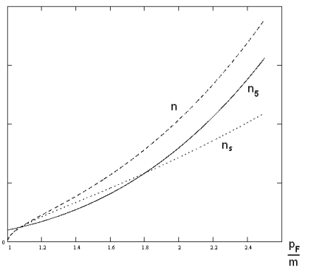
Figure 1: Axial (solid), particle number (dashed) and scalar (dotted) densities of tachyon Fermi gas at zero temperature vs Fermi momentum

References

• [1] A. Sen, Int. J. Mod. Phys. A 18, 4869 (2003); arXiv:hep-th/0209122. M. C. Bento, O. Bertolami, and A. A. Sen, Phys. Rev. D 67, 063511 (2003); arXiv:hep-th/0208124. A. Frolov, L. Kofman, and A. Starobinsky, Phys. Lett. B 545, 8 (2002); arXiv:hep-th/0204187. E. J. Copeland, M. Sami, and S. Tsujikawa, Int. J. Mod. Phys. D 15, 1753 (2006); arXiv:hep-th/0603057. S. Bhattacharya and U. Debnath, Int. J. Theor. Phys. 51, 565 (2012); arXiv:1012.5532.
• [2] L. J. Wang, A. Kuzmich and A. Dogariu, Nature 406, 277 (2000). R.Y. Chiao, A.E. Kozhekin, and G. Kurizki, Phys. Rev. Lett. 77, 1254 (1996). E. Recami, F. Fontana, and R. Garavaglia, Int. J. Mod. Phys. A 15, 2793 (2000); arXiv:0709.2453. Y. Aharonov, B. Reznik, and A. Stern, Phys. Rev. Lett. 81, 2190 (1998); arXiv:quant-ph/9804018. R. G. Ghulghazaryan and Y. P. Malakyan, Phys. Rev. A 67, 063806 (2003); arXiv:physics/0209036.
• [3] A. Chodos, A. I. Hauser, and V. A. Kostelecky, Phys. Lett. B 150, 431 (1985).
• [4] H. M. Fried and Y. Gabellini, Quantum Tachyon Dynamics, arXiv:0709.0414.
• [5] U. D. Jentschura and B. J. Wundt, Symmetries of the Tachyonic Dirac Equation, arXiv:1110.4171
• [6] J. I. Kapusta and C. Gale, Finite-temperature field theory, 2nd ed. (Cambridge Univ. Press, Cambridge, 2004), p. 221.
• [7] T. Chang, A new Dirac-type equation for tachyonic neutrinos, arXiv:hep-th/0011087
• [8] M. I. Park and Y. J. Park, Mod. Phys. Lett. A 12, 2103 (1997); arXiv:hep-th/9510132
• [9] E. Trojan and G. V. Vlasov, Phys. Rev. D 83, 124013 (2011). arXiv:1103.2276
• [10] E. Trojan, Tachyonic Dirac sea, arXiv:1201.6560