Mixed-state quantum transport in correlated spin networks

Abstract

Quantum spin networks can be used to transport information between separated registers in a quantum information processor. To find a practical implementation, the strict requirements of ideal models for perfect state transfer need to be relaxed, allowing for complex coupling topologies and general initial states. Here we analyze transport in complex quantum spin networks in the maximally mixed state and derive explicit conditions that should be satisfied by propagators for perfect state transport. Using a description of the transport process as a quantum walk over the network, we show that it is necessary to phase correlate the transport processes occurring along all the possible paths in the network. We provide a Hamiltonian that achieves this correlation, and use it in a constructive method to derive engineered couplings for perfect transport in complicated network topologies.

I Introduction

In the quest toward a scalable quantum computer Ladd et al. (2010), a promising model comprises distributed computing units connected by passive wires that transmit quantum information Cirac et al. (1999); Oi et al. (2006); Jiang et al. (2007); Kimble (2008); Meter et al. (2008). This architecture would provide several advantages, since the wires require no or limited control, easing the fabrication requirements and improving their isolation from the environment. For a simpler integration in a solid-state architecture, the wires can be composed of spins. Following seminal work by Bose Bose (2003), which showed that spin chains enable transporting quantum states between the ends of the chain, the dynamics of quantum state transfer has been widely studied (see Ref. Kay (2010) for a review) and protocols for improving the fidelity by coupling engineering Christandl et al. (2004); Albanese et al. (2004); Nikolopoulos et al. (2004a, b); Gualdi et al. (2008); Wojcik et al. (2005); Li et al. (2005); Wang et al. (2011), dual-rail topologies Burgarth and Bose (2005), active control on the chain spins Álvarez et al. (2010) or on the end spins only Fitzsimons and Twamley (2006); Burgarth et al. (2007); Caneva et al. (2009); Burgarth et al. (2010) have been proposed. Recently these studies have been extended to mixed state spin chains Cappellaro et al. (2007); DiFranco et al. (2008); Cappellaro et al. (2011); Yao et al. (2011); Kaur and Cappellaro (2011), which are more easily obtained in high-temperature laboratory settings – making them important protagonists in practical quantum computing. A further challenge to experimental implementation of quantum transport is the lack of chains with the desired coupling strengths, since coupling engineering is limited by fabrication constraints and by the presence of long-range interactions. These challenges highlight the need for a systematic study of mixed state transport in quantum systems beyond chains, including more complex network topologies. These topologies reflect more closely actual experimental conditions as well as systems occurring in nature. For example, there is remarkable recent evidence Panitchayangkoon et al. (2011); Engel et al. (2007) that coherent quantum transport may be the underlying reason for the high efficiency (of over 99%) of photosynthetic energy transfer Mohseni et al. (2008).

To derive explicit conditions for perfect transport we quantify geometric constraints on the unitary propagator that drives transport in an arbitrary network. As a consequence, we find that transferring some mixed states in a network in general requires fewer conditions than pure state transfer. Transport conditions for pure states have been previously quantified Kostak et al. (2007), however, our method – relying on decomposing the propagator in orthogonal spaces – is fundamentally different and more suitable for mixed states.

Perfect transport occurs when the bulk of the network acts like a lens to focus transport to its ends. To make this physical picture more concrete, we describe mixed state transport as a continuous quantum walk over the network Aharonov et al. (1993); Baum et al. (1985); Munowitz et al. (1987) that progressively populates its nodes. Through this formalism, we derive constructive conditions on the Hamiltonian that results in the correlation of transport processes through different possible paths in the network. The correlation of transport processes leads to their constructive interference at the position of the two end-spins, giving perfect transport. While similar walk models have been applied to coherent transfer before (see Mülken and Blumen (2011) for a review), our work provides their first extension to transport involving mixed states.

The insight gained by describing quantum transport as correlated quantum walks can be used to construct larger networks where perfect transport is possible. Here we show a strategy to achieve this goal by engineering the coupling strengths between different nodes of the network to construct weighted spin networks that support perfect mixed state transport. Feder Feder (2006) had considered a similar problem for pure states by mapping the quantum walk of $N$ spinor bosons to a single particle; this has been extended in more recent work Krovi and Brun (2007); Bernasconi et al. (2008); Pemberton-Ross and Kay (2011). Here we find far more relaxed weighting requirements for mixed state transport, thanks in part to a fermionic instead of bosonic mapping. In turn, this could ease the fabrication requirements for coupling engineering.

The paper is organized as follows. In Sec. II we define the problem of mixed state transport. Sec. III provides the geometric conditions on the propagator for perfect transport in arbitrary networks. We finally present in Sec. IV the quantum walk formalism, which allows the correlation of transport processes over different paths and the construction of families of weighted networks that support perfect transfer.

II Transport in mixed-state networks

Consider an $N$-spin network ${\cal N}$, whose vertices (nodes) ${\cal V}$ represent spins and whose edges ${\cal E}=\{\alpha_{ij}\}$ describe the couplings between spins $i$ and $j$ (see Fig. 1). The system dynamics is governed by the Hamiltonian $H=\sum_{i<j}\alpha_{ij}H_{ij}$, where $H_{ij}$ is the operator form of the interaction. In the most general case, a spin of ${\cal N}$ may be coupled to several others, for instance, in a dipolar coupled network, $\alpha_{ij}\sim 1/r_{ij}^{3}$ is a function of the distance between the spins in the network.

We assume that we can identify two nodes, labeled 1 and $N$, that we can (partially) control and read out, independently from the “bulk” of the network, and thus act as the “end” spins between which transport will occur. The rest of the spins in the network can at most be manipulated by collective control. This also imposes restrictions on the network initialization DiFranco et al. (2008); Cappellaro et al. (2011); Yao et al. (2011). To relax the requirements for the network preparation, we assume to work in the infinite-temperature limit Cappellaro et al. (2011) – a physical setting easily achievable for many experimental systems – where the bulk spins are in the maximally mixed state, $\rho\propto\openone$. We will then consider the transport of a slight excess polarization from node $1$ to node $N$. The initial state is $\rho_{i}\sim(\openone+\delta Z_{1})$, where $Z_{1}$ is the Pauli matrix acting on spin 1 and $\delta\ll 1$ denotes the polarization excess. Since only the traceless part of the density matrix evolves in time, we will monitor the transport from $\rho^{\Delta}_{i}=Z_{1}$ to a desired final state $\rho^{\Delta}_{f}=Z_{N}$. The fidelity of the transport process is then defined as $F(t)={\rm Tr}(\rho^{\Delta}(t)Z_{N})/{\rm Tr}(Z^{{\dagger}}_{1}Z_{1})$, with $\rho^{\Delta}(t)=U(t)\rho^{\Delta}_{i}U^{\dagger}(t)$ being the evolved state.

The polarization behaves like a wave-packet traveling over the network ${\cal N}$ Osborne and Linden (2004); Yung (2006). In most cases, the Hamiltonian $H$ drives a rapidly dispersive evolution, where the wave-packet quickly spreads out into many-body correlations among the nodes of ${\cal N}$, from which it cannot be recovered Munowitz et al. (1987). This is for example the case of evolution under the naturally occurring dipolar Hamiltonian, which induces a fast-decay of the spin polarization as measured in solid-state NMR, even if many-body correlations can be detected at longer times Cho et al. (2005).

In order to drive a dispersionless transport, thus ensuring perfect fidelity, the network Hamiltonian should satisfy very specific conditions. In this paper we will investigate these conditions by answering the questions: (i) What are the possible operator forms of the Hamiltonian $H_{ij}$ for dispersionless transport? (ii) What are the coupling topologies and (iii) strengths $\alpha_{ij}$ that support perfect transport?

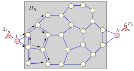
Figure 1: (Color online) Transport in a spin network. The network edges represent the interaction among spins (nodes). The pink (dark) nodes represent the end spins between which transport should occur. The shaded region comprising yellow (light) nodes is the bulk network, $H_{B}$. An initial polarization packet (hatched) is prepared on spin 1 and allowed to propagate on the network through various possible paths (arrows). For perfect transport, the polarization refocuses at spin $N$.

III Conditions for perfect transport

III.1 Fidelity of mixed-state transport

The condition for perfect transport, $F=1$, can be expressed in a compact form by using the product-operator (PO) basis Sorensen et al. (1984). For the $N$-spin network system there are $2^{2N}$ basis elements,

$$\textbf{B}=\textbf{B}_{1}\otimes\textbf{B}_{\textrm{bulk}}\otimes\textbf{B}_{N}=\{\openone,X_{1},Y_{1},Z_{1},X_{2},\dots,X_{1}X_{2},$$

$$\dots,Z_{1}Z_{2},X_{1}X_{2}X_{3},\dots,\dots,Z_{1}Z_{2}\cdots Z_{N-1}Z_{N}\},$$ (1)

where $\textbf{B}_{1,N}$ and $\textbf{B}_{\textrm{bulk}}$ are the basis for the end and the bulk spins, respectively.

Using the PO basis, the propagator $U(t)=e^{-iHt}$ can be represented by a vector $\left|{U}\right\rangle=[c_{B_{1}},c_{B_{2}},\dots,c_{B_{4^{N}}}]^{T}$ in the $2^{2N}$ dimensional Hilbert-Schmidt (HS) operator space spanned by B Ajoy et al. (2012):

$$U(t)=\textstyle\sum_{i}c_{B_{i}}(t)B_{i},\quad{\rm with}\quad c_{B_{i}}=\displaystyle\frac{\textrm{Tr}(B_{i}^{\dagger}U)}{\textrm{Tr}(B_{i}^{\dagger}B_{i})}$$

From an initial state with a polarization excess on spin 1, $\rho_{i}^{\Delta}=Z_{1}$, the system evolves to

$$\rho^{\Delta}_{f}=U\rho^{\Delta}_{i}U^{\dagger}=\textstyle\sum_{i,j}c_{B_{i}}c_{B_{j}}^{\ast}B_{i}Z_{1}B_{j}\>,$$ (2)

yielding the transport fidelity to spin $N$

$$F \!=\! \frac{1}{{\rm Tr}(Z^{{\dagger}}_{1}Z_{1})}\textrm{Tr}\left[\textstyle\sum_{i,j}c^{\ast}_{B_{i}}c_{B_{j}}B_{i}Z_{1}B_{j}Z_{N}\right]\!\!=\!\textstyle\sum_{i}c_{B_{i}}c_{B_{j}}^{\ast},$$ (3)

$${\rm with}\ B_{j}=\pm Z_{1}Z_{N}B_{i},\quad{\rm for}\quad[B_{i},Z_{N}]_{\mp}=0.$$

The last equation follows from the property that all elements of B, except $\openone$, are traceless.

The fidelity derived in Eq. (3) has a simple form in the HS space. Note that in this operator space, the product $B_{i}U$ is a linear transformation, $\textbf{T}:\left|{U}\right\rangle\rightarrow\hat{P}_{B_{i}}\left|{U}\right\rangle$, where $\hat{P}_{B_{i}}$ is a permutation matrix corresponding to the action of $B_{i}$ Ajoy et al. (2012) (here and in the following we denote operators in the HS space by a hat). The unitarity of $U$ yields the conditions:

$$\|{U}\|=\langle{U}|{U}\rangle=1\qquad\left\langle{U}\right|\hat{P}_{B_{i}}\left|{U}\right\rangle=0\>,\>B_{i}\neq\openone.$$ (4)

Let us partition the HS space in two subspaces $\cal G$, $\widetilde{\cal G}$, spanned by the basis $G$ and $\widetilde{G}$,

$${G}=\textbf{B}_{1}\otimes\textbf{B}_{\rm bulk}\otimes\{\openone,Z_{N}\},\quad\widetilde{G}=\textbf{B}_{1}\otimes\textbf{B}_{\rm bulk}\otimes\{X_{N},Y_{N}\},$$

and note that all elements of ${G}$ commute with $Z_{N}$, while all elements of $\widetilde{G}$ anti-commute with $Z_{N}$. We will label by superscripts ${{\cal G}}$ and ${\widetilde{\cal G}}$ the projections of operators in these subspaces. Using this partition, we can simplify the expression for the fidelity of Eq. (3) to obtain

$$F=\left\langle{U}\right|\hat{P}_{Z_{1}Z_{N}}\hat{P}_{R}\left|{U}\right\rangle\>,$$ (5)

where $\hat{P}_{R}$ is a reflection about ${\cal G}$ and $\hat{P}_{Z_{1}Z_{N}}$ is block-diagonal in the $\{{G},\widetilde{{G}}\}$ basis (since $Z_{1}Z_{N}\in{\cal G}$):

$$\hat{P}_{R}=\left[\begin{array}[]{cc}\openone^{\cal G}&0\\ 0&-\openone^{\widetilde{\cal G}}\\ \end{array}\right],\quad\hat{P}_{Z_{1}Z_{N}}=\left[\begin{array}[]{cc}\hat{P}_{Z_{1}Z_{N}}^{\cal G}&0\\ 0&\hat{P}_{Z_{1}Z_{N}}^{\widetilde{\cal G}}\\ \end{array}\right]$$ (6)

Rewriting the fidelity as the inner product between two vectors, $F=\langle{(\hat{P}_{Z_{1}Z_{N}}U)}|{\hat{P}_{R}{U}}\rangle$, provides a simple geometric interpretation of the perfect transport condition, as shown in Fig. 2. The vector $\hat{P}_{Z_{1}Z_{N}}\left|{U}\right\rangle$ should be parallel to $\hat{P}_{R}\left|{U}\right\rangle$, which can be obtained if $\hat{P}_{Z_{1}Z_{N}}$ rotates $\left|{U^{\widetilde{{\cal G}}}}\right\rangle$ by an angle $\pi$, while leaving $\left|{U^{{\cal G}}}\right\rangle$ unaffected. Alternatively, since $\hat{P}_{Z_{1}Z_{N}}$ just describes a $\pi-$rotation of the vector $\left|{U}\right\rangle$ about the $Z_{1}Z_{N}$ axis, for perfect transport the rotation-reflection operation $\hat{S}=\hat{P}_{Z_{1}Z_{N}}\hat{P}_{R}$ should be a symmetry operation for $\left|{U}\right\rangle$.

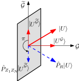
Figure 2: (Color online) Geometric interpretation of the condition for maximum $Z_{1}\rightarrow Z_{N}$ transport fidelity. The unitary $U$ is represented as a vector $\left|{U}\right\rangle$ (red thick arrow) in the HS space, with components $\left|{U^{\cal G}}\right\rangle$ and $\left|{U^{\widetilde{\cal G}}}\right\rangle$ in the subspaces ${\cal G}$ (represented by an axis) and $\widetilde{\cal G}$ (represented by the shaded grey plane). $\hat{P}_{R}\left|{U}\right\rangle$ (blue dashed arrow) is the reflection of $\left|{U}\right\rangle$ about the ${\cal G}$ axis. Maximum fidelity occurs only when the $\hat{P}_{Z_{1}Z_{N}}$ causes a $\pi$-rotation of $\left|{U^{\widetilde{\cal G}}}\right\rangle$.

From Eq. (4) we have $\left\langle{U}\right|\hat{P}_{Z_{1}Z_{N}}\left|{U}\right\rangle=0$ and using Eq. (5) we can derive explicit conditions to be satisfied by the propagator to achieve perfect transport, $F=1$

$$\left\langle{U^{\cal G}}\right|\hat{P}_{Z_{1}Z_{N}}^{\cal G}\left|{U^{\cal G}}\right\rangle+\left\langle{U^{\widetilde{{\cal G}}}}\right|\hat{P}_{Z_{1}Z_{N}}^{\widetilde{\cal G}}\left|{U^{\widetilde{{\cal G}}}}\right\rangle = 0$$ (7)

$$\left\langle{U^{\cal G}}\right|\hat{P}_{Z_{1}Z_{N}}^{\cal G}\left|{U^{\cal G}}\right\rangle-\left\langle{U^{\widetilde{{\cal G}}}}\right|\hat{P}_{Z_{1}Z_{N}}^{\widetilde{\cal G}}\left|{U^{\widetilde{{\cal G}}}}\right\rangle = 1$$ (8)

that simplify to

$$\left\langle{U^{\cal G}}\right|\hat{P}_{Z_{1}Z_{N}}^{\cal G}\left|{U^{\cal G}}\right\rangle=-\left\langle{U^{\widetilde{{\cal G}}}}\right|\hat{P}_{Z_{1}Z_{N}}^{\widetilde{\cal G}}\left|{U^{\widetilde{{\cal G}}}}\right\rangle=\frac{1}{2}\>.$$ (9)

When is this equation satisfied? By symmetry, it happens when $\|{U}^{\cal G}\|=\|{U}^{\widetilde{{\cal G}}}\|=1/2$, and $\left|{U^{\cal G}}\right\rangle$ and $\left|{U^{\widetilde{{\cal G}}}}\right\rangle$ are (up to a phase) eigenvectors of $\hat{P}_{Z_{1}Z_{N}}^{\cal G}$ and $\hat{P}_{Z_{1}Z_{N}}^{\widetilde{\cal G}}$ with eigenvalues $\pm 1$ respectively:

$$\hat{P}_{Z_{1}Z_{N}}^{\cal G}\left|{U^{\cal G}}\right\rangle=+\left|{U^{\cal G}}\right\rangle;\quad\hat{P}_{Z_{1}Z_{N}}^{\widetilde{\cal G}}\left|{U^{\widetilde{\cal G}}}\right\rangle=-\left|{U^{\widetilde{{\cal G}}}}\right\rangle$$ (10)

To enable perfect transport, $\left|{U}\right\rangle$ must thus have an equal projection on the two subspaces ${\cal G}$ and $\widetilde{{\cal G}}$, as shown geometrically in Fig. 2. Also, intuitively from the symmetry operation $\hat{S}$, all components of $\left|{U}\right\rangle$ lying on the plane ${\cal G}$ should be rotationally symmetric with respect to $Z_{1}Z_{N}$, while components of $\left|{U}\right\rangle$ lying on the plane $\widetilde{\cal G}$ should have reflection symmetry about $Z_{1}Z_{N}$.

Note that Eq. (10) imposes fairly weak constraints on the transport unitaries, as opposed to the constraints for pure state transport Kostak et al. (2007); Karbach and Stolze (2005). In particular Eq. (10) provides no explicit constraint on the bulk of the network. For example, the two propagators,

$$\begin{array}[]{l}U_{1}=B_{\rm bulk}(\openone\pm Z_{1}Z_{N})+B_{\rm bulk}^{{}^{\prime}}(X_{1}X_{N}\pm Y_{1}Y_{N}),\\ U_{2}=B_{\rm bulk}(\openone\pm Z_{1}Z_{N})+B_{\rm bulk}^{{}^{\prime}}(X_{1}Y_{N}\mp Y_{1}X_{N}),\end{array}$$ (11)

with $B_{\rm bulk}$ and $B_{\rm bulk}^{{}^{\prime}}$ arbitrary equi-norm operators ($\in{\rm span}\{\bf{B}_{\rm bulk}\}$) acting on the bulk, support perfect transport. Other propagators can be obtained thanks to an invariance property that we present in the next section. More generally, in Appendix A we explicitly provide a prescription to construct classes of unitaries for perfect mixed state transport.

III.2 Invariance of transport Hamiltonians

The fidelity $F$ in Eq. (3) is invariant under a transformation $U^{{}^{\prime}}=VU$, where $V$ is unitary and commutes with $\hat{S}$, that is,

$$[\hat{V},\hat{P}_{Z_{1}Z_{N}}\hat{P}_{R}]=0.$$ (12)

This invariance can be used to construct Hamiltonians that support perfect transport starting from known ones. Consider an Hamiltonian $H$ that generates the transport evolution $U=\exp(-iHt)$. Then the transport driven by $H$ is identical to that generated by the Hamiltonian $H^{{}^{\prime}}=V^{\dagger}HV$, where $V$ satisfies Eq. (12).

Ref. Kay (2011) proved similar symmetry requirements for Hamiltonians that transport pure states; here, however, we derived these Hamiltonian properties just from the geometric conditions on $U$. Ref. Hincks et al. (2011) treated a similar problem, defining classes of Hamiltonians that perform the same action on a state of interest. A special case of this result was used in Cappellaro et al. (2007) to study transport in a mixed-state spin chain driven either by the nearest-neighbor coupling isotropic XY Hamiltonian,

$$H_{\rm XY}=\textstyle\sum_{i}\alpha_{i}T_{ii+1}^{+}\text{ with }T_{ij}^{+}=(S_{i}^{+}S_{j}^{-}+S_{i}^{-}S_{j}^{+})$$ (13)

or double-quantum (DQ) Hamiltonian

$$H_{\rm DQ}=\textstyle\sum_{i}\alpha_{i}D_{ii+1}^{+}\text{ with }D_{ij}^{+}=(S_{i}^{+}S_{j}^{+}+S_{i}^{-}S_{j}^{-}),$$ (14)

with $S_{j}^{\pm}=\frac{1}{2}(X_{j}\pm iY_{j})$. The unitary operator relating the two Hamiltonians, $V=\prod_{k^{{}^{\prime}}}X_{k^{{}^{\prime}}}$, where the product $k^{{}^{\prime}}$ extends over all even or odd spins, does indeed satisfy Eq. (12).

III.3 Quantum information transport via mixed state networks

The requirements for perfect transport (Eq. (10)) can be easily generalized to the transport between any two elements of B, say from ${\cal I}$ to ${\cal F}$. One has simply to appropriately construct the subspaces ${\cal G}$ and $\widetilde{\cal G}$ and the corresponding permutation operator $\hat{P}_{{\cal IF}}$.

One could further consider under which conditions this transport (for example, $X_{1}\rightarrow X_{N}$) can occur simultaneously with the $Z_{1}\rightarrow Z_{N}$ transport already considered. More generally, the simultaneous transfer of operators forming a basis for $\bf{B_{1}}$ would enable the transport of quantum information Cappellaro et al. (2011); Albanese et al. (2004) via a mixed-state network. The unitary $U$ should now not only be symmetric under $\hat{S}$, but should also under a similar operator derived for $X_{1}X_{N}$. The requirements on $U$ thus become more stringent and only a special case of the propagators constructed in Eq. (LABEL:eqn:A1.1) in Appendix A is allowed,

$$U=B_{\rm bulk}(\openone\pm Z_{1}Z_{N}+X_{1}X_{N}\pm Y_{1}Y_{N})\>.$$ (15)

This is exactly a SWAP operation (up to a phase) between the end-spins, which can also lead to a transfer of arbitrary pure states between $1$ and $N$. Therefore, we find that perfect transport of non-commuting mixed states between the end-spins also allows transport in pure state networks. We note that quantum information could be encoded in multi-spin states Markiewicz and Wiesniak (2009); Cappellaro et al. (2011) that satisfy proper symmetry conditions and thus do not impose additional conditions on the transport propagators.

III.4 Which Hamiltonians support mixed state transport?

It would be interesting to determine which Hamiltonians can generate propagators $\left|{U(t)}\right\rangle=\exp(-i\hat{H}t)\left|{\openone}\right\rangle$ for perfect transport. Unfortunately, deriving requirements for the Hamiltonian from the conditions on the unitaries is non-trivial; however, as we show below, one can still extract useful information.

A general Hamiltonian can be decomposed as $H=H^{{\cal G}}+H^{\widetilde{{\cal G}}}$, where $H^{{\cal G},\widetilde{{\cal G}}}$ lie in the subspaces ${\cal G}$ and $\widetilde{{\cal G}}$, respectively. We cannot set $H=H^{{\cal G}}$ since the Hamiltonian does need to have a component that is non-commuting with the target operator ($Z_{N}$) in order to drive the transport. If $H=H^{\widetilde{\cal G}}$, odd powers of $H$ are in $\widetilde{{\cal G}}$, while even powers of $H$ belong to ${{\cal G}}$. Then the propagator has contributions from $\left|{U^{\cal G}}\right\rangle$ and $\left|{U^{\widetilde{\cal G}}}\right\rangle$ with

$$\left|{U^{{\cal G}}}\right\rangle = \left|{\openone}\right\rangle+\frac{(it)^{2}}{2!}\hat{H}\left|{H}\right\rangle+\frac{(it)^{4}}{4!}\hat{H}^{3}\left|{H}\right\rangle+\cdots$$

$$\left|{U^{\widetilde{{\cal G}}}}\right\rangle = it\left|{H}\right\rangle+\frac{(it)^{3}}{3!}\hat{H}^{2}\left|{H}\right\rangle+\cdots$$ (16)

We can demonstrate that in this case the Hamiltonian must satisfy two conditions to drive perfect transport. First, the “vector” form of the Hamiltonian must be an eigenstate of $\hat{P}_{Z_{1}Z_{N}}$, $\hat{P}_{Z_{1}Z_{N}}\left|{H}\right\rangle=-\left|{H}\right\rangle$, which ensures that the second equation in (10) is trivially satisfied, as $\hat{P}_{Z_{1}Z_{N}}\left|{U^{\widetilde{\cal G}}}\right\rangle=-\left|{U^{\widetilde{\cal G}}}\right\rangle$. Second, since we have

$$\hat{P}_{Z_{1}Z_{N}}\left|{U^{{\cal G}}}\right\rangle=\left|{Z_{1}Z_{N}}\right\rangle+\frac{(it)^{2}}{2!}\hat{H}\left|{H}\right\rangle+\frac{(it)^{4}}{4!}\hat{H}^{3}\left|{H}\right\rangle+\cdots,$$

the first equation in (10) implies that $H^{2n}\!=\!\frac{1}{2}(\openone\!-\!Z_{1}Z_{N})$ for any $n$.

These conditions are for example satisfied by the XY-like Hamiltonian, $H=B_{\rm bulk}T_{1N}^{+}$, where $B_{\rm bulk}$ is any operator acting on the bulk and $T_{1N}^{\pm}=(S_{1}^{+}S_{N}^{-}\pm S_{1}^{-}S_{N}^{+})$. In this case, at $t=\pi/4$, all conditions in Eq. (10) are satisfied and perfect transport is achieved. Indeed the XY Hamiltonian has been widely studied for quantum transport Bose (2003); Christandl et al. (2004) and it is interesting that we could derive its transport properties solely by the symmetry conditions on the propagator.

An Hamiltonian $H=H^{\widetilde{\cal G}}$ with support only in $\widetilde{\cal G}$ is however a very restrictive case as it refers to the situation where all nodes of the network are connected to $N$. Hamiltonians with support in both subspaces are more experimentally relevant, as they correspond to a common physical situation, where the ends of the network are separated in space and direct interaction between them is zero or too weak. In the following, we will consider this more general situation, although restricting the study to XY Hamiltonians in order to derive conditions for perfect transport.

IV Perfect Transport in networks: Correlated Quantum walks

In the following, we will consider the network ${\cal N}$ to consist of spins that are coupled by XY-like interaction, $\{T_{ij}^{+}\}$. We focus on this interaction since it has been shown that with appropriate engineered coupling strengths, $\alpha_{ij}\propto\sqrt{i(N-i)}\delta_{j,i+1}$, the XY-Hamiltonian can support perfect transport in linear spin chains (see e.g. Nikolopoulos et al. (2004a, b); Albanese et al. (2004); Benjamin and Bose (2003)). Thanks to the invariance property described in Sec. III.2, this analysis applies to a much broader class of Hamiltonians, in particular to the DQ Hamiltonian.

We assume that the end spins of ${\cal N}$ are not directly coupled, thus transport needs to be mediated by the bulk of the network. The simplest such topology is a $\Lambda$-type configuration where the end spins are coupled to a single spin in the bulk. The Hamiltonian $\Lambda_{j}=(T_{1j}^{+}+T_{jN}^{+})/\sqrt{2}$, where $j$ is a spin in the bulk, is enough to drive this transport. In this case, $(\Lambda_{j}^{2})^{n}\!=\!\Lambda_{j}^{2}\ \forall\,n$, and hence the propagator is

$$U=\exp(-iHt)=\openone+[\cos(t)-1]H^{2}-i\sin(t)H,$$ (17)

where $H^{2}=1/2[(T_{1j}^{+})^{2}+(T_{jN}^{+})^{2}+T_{1N}^{+}]$. Since $(\openone-2H^{2})$ has the form of $U_{3}$ in Eq. (LABEL:eqn:A1.1), setting $t=\pi$ ensures $U=U_{3}$, yielding perfect transport. This is an expected result, since this simple lambda-network is just a 3-spin linear chain. This result can be extended to longer chains, as long as engineered couplings ensure that the resulting Hamiltonian is mirror-symmetric Karbach and Stolze (2005); Albanese et al. (2004); Wang et al. (2011).

A different situation arises when there is more than one transport path possible, that is, the end spins are coupled to more than one spin in the bulk with an Hamiltonian $H=\sum_{j\in\rm{bulk}}\alpha_{j}\Lambda_{j}$. For example, Fig. 3 depicts a network similar to the one considered in Yao et al. (2011); Clark et al. (2005) where there are three $\Lambda$ paths between the end-spins. Even if each path individually supports perfect transport, evolution along different paths may not be correlated, leading to destructive interference reducing the fidelity (see Fig. 3).

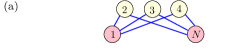
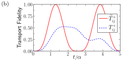
Figure 3: (Color online) (a) $\Lambda$-type network with three $\Lambda$ paths between the bulk and end-spins and equal coupling strength $\alpha$. (b) Transport fidelity as a function of normalized time for the $\Lambda$-network coupled by the XY-Hamiltonian $T_{ij}^{+}$ (blue dashed) and the modified XY-Hamiltonian $\widetilde{T}_{ij}^{+}$ (red solid). In the latter case, correlated quantum walks lead to perfect transport.

Perfect fidelity can be achieved only if different paths can be collapsed into a single “effective” one that supports perfect transport (Fig. 8). This strategy not only allows us to determine if an Hamiltonian can support perfect transport, but it also gives a recipe to build allowed Hamiltonians, by combining simpler networks known to support perfect transport into more complex ones.

To this end, we use the fact that linear chains enable perfect transport with appropriate engineered couplings. Our first step will then to give conditions under which two chains of the same length (with end-spins in common) can be combined. To obtain these conditions, we describe the evolution of the spin polarization as a quantum walk over the operators in the network Baum et al. (1985); Munowitz et al. (1987). This description reveals the need to correlate the parallel paths over the network, in order to achieve a constructive refocusing of the polarization at the other end of the network. We then generalize the conditions by a recursive construction to quite general networks.

IV.1 Transport as a quantum walk over ${\cal N}$

We describe the transport evolution as a quantum walk over the network, which progressively populates operators in the HS space. This process of progressively populating different parts of the HS space upon continuous time evolution under the Hamiltonian can be considered as a quantum walk Baum et al. (1985); Munowitz et al. (1987); Di Franco et al. (2007). We first expand the transport fidelity $F(t)$ (Eq. 5) in a time series,

$$F(t) = \left\langle U_{0}\left|\hat{P}_{Z_{1}Z_{N}}\hat{P}_{R}\right|U_{0}\rangle-it\langle U_{0}\left|[\hat{H},\hat{P}_{Z_{1}Z_{N}}\hat{P}_{R}]\right|U_{0}\right\rangle$$ (18)

$$+ \frac{i^{2}t^{2}}{2!}\left\langle U_{0}\left|\left[\hat{H},\left[\hat{H},\hat{P}_{Z_{1}Z_{N}}\hat{P}_{R}\right]\right]\right|U_{0}\right\rangle+\cdots$$

with $|U_{0}\rangle=\left|{\openone}\right\rangle$. Defining the nested commutators,

$${\cal C}_{0}=\hat{P}_{Z_{1}Z_{N}}\hat{P}_{R}\ ;\ {\cal C}_{n}=[\hat{H},{\cal C}_{n-1}]\>,$$ (19)

Eq. (18) takes the form

$$F(t)=\sum_{n=0}^{\infty}\frac{(it)^{n}}{n!}\langle{\cal C}_{n}\rangle,$$ (20)

where the expectation value is taken with respect to $\left|{{U}_{0}}\right\rangle$.

A large part of the Hamiltonian commutes with $\hat{P}_{Z_{1}Z_{N}}\hat{P}_{R}$ and can be neglected. We can isolate the non-commuting part by defining the operator $\hat{A}$ via the relationship

$$[\hat{H},\hat{P}_{Z_{1}Z_{N}}\hat{P}_{R}]=\hat{A}\hat{P}_{Z_{1}Z_{N}}\hat{P}_{R}\>.$$ (21)

The operator $\hat{A}$ and its nested commutators ${\cal C}_{n}^{A}=[\hat{H},{\cal C}_{n-1}^{A}]$ (with ${\cal C}_{0}^{A}=\hat{A}$) have a simple graphical construction. The commutation relations,

$$\left[{T}_{ij}^{+},{T}_{jk}^{\pm}\right]=-Z_{j}{T}_{ik}^{\mp};\qquad\left[{T}_{ij}^{+},{T}_{kl}^{+}\right]=0\,,$$ (22)

(see Fig. 4) can be used to provide a simple prescription to graphically determine the flip-flop terms in ${\cal C}_{n}^{A}$.

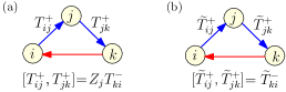
Figure 4: (Color online) Graphical representation of commutators for (a) the XY and (b) the modified XY Hamiltonian. The commutator between two top legs (blue) of the directed graph is the third edge (red). In case of the XY Hamiltonian, the commutator is conditioned on node $j$.

For any two edges, one in ${\cal C}_{n-1}^{A}$ and one in $H$, that share a common node, ${\cal C}_{n}^{A}$ contains the edge required to complete the triangle between them. Thus, each higher order in the commutation expansion creates a link between nodes in the network, progressively populating it. We will refer to the operators ${\cal C}_{n}^{A}$ as quantum walk operators, since as we show below, the nested commutators ${\cal C}_{n}$ in Eq. (20) can be built exclusively out of them.

Consider the network of Fig. 5(a), with coupling strengths $\alpha_{ij}=1$: $\hat{A}$ contains only the edges of ${\cal N}$ that connect to node $1$, as represented by the red lines in Fig. 5(b).

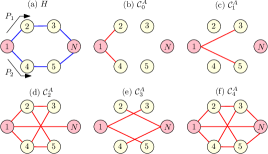
Figure 5: (Color online) (a) A six spin network with two paths $P_{1}$ and $P_{2}$ between the end spins. (b)-(f) represent graphically the successive orders of the quantum walk operators ${\cal C}_{n}^{A}$: A red line linking two nodes indicates that there is a flip-flop term $T_{ij}^{\pm}$ between them, while path-dependent prefactors are not depicted. Once the walk has covered the entire network, successive orders in ${\cal C}_{n}^{A}$ reproduce ${\cal C}_{3}^{A}$ and ${\cal C}_{4}^{A}$. The explicit expressions for the commutators are shown in Table 1.

Fig. 5(c-d) represent the higher order commutators, with a red line linking two nodes denoting a term $T_{ij}^{\pm}$ between them. We note that the graphical construction only predicts the presence of a flip-flop term $T_{ij}^{\pm}$ linking two nodes in the commutator ${\cal C}_{n}^{A}$, while the explicit forms of the commutators is generally more complex, as shown in Table 1, with additional appropriate weights for arbitrary coupling strengths $\alpha_{ij}$. Still, as we now show, only the $T_{ij}^{\pm}$ terms are important to determine the fidelity, and the presence of a $T_{1N}^{\pm}$ term in the graphical series is an indication that transport can occur between the end-nodes.

The commutators ${\cal C}_{n}$ can indeed be written in terms of the ${\cal C}_{n}^{A}$ nested commutators,

$${\cal C}_{n}=\sum_{k=0}^{n-1}\dbinom{n-1}{k}{\cal C}_{n-1-k}^{A}{\cal C}_{k},$$ (23)

yielding an expression for the fidelity containing only products of the nested commutators ${\cal C}_{n}^{A}$:

$${\cal C}_{n}=\sum_{k_{1}=0}^{n-1}\sum_{k_{2}=0}^{k_{1}-1}\cdots\sum_{k_{n}=0}^{k_{n-1}-1}\dbinom{n-1}{k_{1}}\dbinom{k_{1}-1}{k_{2}}\cdots\dbinom{k_{n-1}-1}{k_{n}}{\cal C}_{n-k_{1}-1}^{A}{\cal C}_{k_{1}-k_{2}-1}^{A}\cdots{\cal C}_{k_{n-1}-k_{n}-1}^{A}\hat{P}_{Z_{1}Z_{N}}\hat{P}_{R}\>.$$ (24)

For a commutator ${\cal C}_{n}$ to yield a non-zero contribution to the fidelity, the product of the operators ${\cal C}_{k}^{A}$ should be proportional to $Z_{1}Z_{N}$, that is, it should evaluate to even powers of $T_{1N}^{\pm}$. Hence very few terms appearing in Eq. (24) actually contribute to the transfer fidelity $F$.

Walk Operator	XY Hamiltonian	Modified XY Hamiltonian
${\cal C}_{0}^{A}$	$T_{12}^{+}+T_{14}^{+}$	$\widetilde{T}_{12}^{+}+\widetilde{T}_{14}^{+}$
${\cal C}_{1}^{A}$	$Z_{2}T_{13}^{-}+Z_{4}T_{15}^{-}$	$\widetilde{T}_{13}^{-}+\widetilde{T}_{15}^{-}$
${\cal C}_{2}^{A}$	$T_{12}^{+}-T_{23}^{+}-Z_{1}Z_{2}T_{34}^{+}+Z_{2}Z_{3}T_{1N}^{+}$	$\widetilde{T}_{12}^{+}-\widetilde{T}_{23}^{+}-\widetilde{T}_{34}^{+}+\widetilde{T}_{1N}^{+}$
	$+T_{14}^{+}-T_{45}^{+}-Z_{1}Z_{4}T_{25}^{+}+Z_{4}Z_{5}T_{1N}^{+}$	$+\widetilde{T}_{14}^{+}-\widetilde{T}_{45}^{+}-\widetilde{T}_{25}^{+}+\widetilde{T}_{1N}^{+}$
${\cal C}_{3}^{A}$	$(Z_{4}Z_{5}Z_{N}+4Z_{2})T_{13}^{-}+(Z_{2}Z_{3}Z_{N}+4Z_{4})T_{15}^{-}$	$5\widetilde{T}_{13}^{-}-4\widetilde{T}_{2N}^{-}$
	$-2(Z_{1}Z_{4}Z_{5}+Z_{3})T_{2N}^{-}-2(Z_{1}Z_{2}Z_{3}+Z_{5})T_{4N}^{-}$	$+5\widetilde{T}_{15}^{-}-4\widetilde{T}_{4N}^{-}$
	$(4\openone+Z_{3}Z_{4}Z_{5}Z_{N})T_{12}^{+}+(4\openone+Z_{2}Z_{3}Z_{5}Z_{N})T_{14}^{+}+9(Z_{2}Z_{3}+Z_{4}Z_{5})T_{1N}^{+}$	$5\widetilde{T}_{12}^{+}+5\widetilde{T}_{14}^{+}+18\widetilde{T}_{1N}^{+}$
${\cal C}_{4}^{A}$	$-(6\openone+3Z_{1}Z_{4}Z_{5}Z_{N})T_{23}^{+}-(6Z_{1}Z_{4}+3Z_{3}Z_{N})T_{25}^{+}-(6Z_{1}Z_{2}+3Z_{5}Z_{N})T_{34}^{+}$	$-9\widetilde{T}_{23}^{+}-9\widetilde{T}_{25}^{+}-9\widetilde{T}_{34}^{+}$
	$+2(\openone+Z_{1}Z_{2}Z_{4}Z_{5})T_{36}^{+}-(6\openone+3Z_{1}Z_{2}Z_{3}Z_{N})T_{45}^{+}+2(\openone+Z_{1}Z_{2}Z_{3}Z_{4})T_{56}^{+}$	$+4\widetilde{T}_{36}^{+}-9\widetilde{T}_{45}^{+}+4\widetilde{T}_{56}^{+}$

Table 1: Nested commutators ${\cal C}_{n}^{A}$ (walk operators) corresponding to the graphs in Fig. 5 if the edges represent the XY Hamiltonian or the modified XY Hamiltonian. In the first case, note the presence of path dependent $Z_{j}$ prefactors, which are absent if the modified XY Hamiltonian is used. This allows for the correlation of transport through parallel paths.

The geometric construction of ${\cal C}_{n}^{A}$ only yields the XY operators contained in each commutator, but it does not reflect the appearance of prefactors $\propto Z_{j}$ (due to the commutator in Eq. (22)) that are explicitly written out in Table 1. Thus, the geometric construction gives a necessary condition for transport, but not a sufficient one.

The operators ${\cal C}_{n}^{A}$ describe the sum of walks over different paths: for example in ${\cal C}_{2}^{A}$, $Z_{2}Z_{3}T_{1N}^{+}$ can be interpreted as the information packet reaching node $N$ through path $P_{1}$ in Fig. 5(a), while $Z_{4}Z_{5}T_{1N}^{+}$ represents propagation via path $P_{2}$. These two terms could in principle contribute to the fidelity, as they contain $T_{1N}^{+}$. However, the additional path dependent factors $\prod_{k}Z_{k}$ lead to a loss of fidelity. Transport through different paths yield different $\prod_{k}Z_{k}$ factors, resulting into a destructive “interference” effect. Note also that since different paths are weighted by different correlation factors, they cannot be canceled through some external control to recover the fidelity. In the following section we show how a modified Hamiltonian can remove this path-conditioning and thus drive perfect transport. Note that the path-dependent factors are as well unimportant in the case of pure states, provided the states reside in the same excitation manifold Clark et al. (2007); Di Franco et al. (2009); Cappellaro et al. (2011).

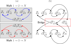
Figure 6: (Color online) Operators appearing in the quantum walk of a network consisting of two $\Lambda$ paths, $1\to 2\to N$ and $1\to 3\to N$. In panel (a), where the transport is driven by the XY-Hamiltonian, the two paths through spins $2$ and $3$ are different, as they traverse a different set of operators, and are thus depicted in two separated grey panels. In panel (b), where we consider the modified XY Hamiltonian, both walks go through a common set of operators. The previously separate walks are bridged by the operators in the red box, making both walks indistinguishable and hence correlated.

IV.2 Correlating quantum walks over ${\cal N}$: Modified XY-Hamiltonian

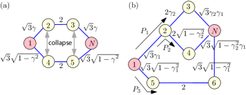
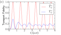
Figure 7: (Color online) Engineered spin networks. (a) The network of Fig. 5(a), correlated by means of the modified flip-flop Hamiltonian, can be engineered to yield perfect transport by weighting the coupling strength $\alpha$ with the coefficient shown. Here $\gamma$ is any positive parameter, $\gamma<1$. The two paths $P_{1}$ and $P_{2}$ can be collapsed to form a linear chain, since nodes $(2,4)$ and $(3,5)$ are equivalent. (b) A more complicated network consisting of three paths $P_{1}-P_{3}$ (black arrows), with engineered strengths parametrized by $0<\gamma_{1},\gamma_{2}<1$. The three paths can be collapsed into an effective 4-spin linear chain, with equivalent nodes (2,5) and (3,4,6). (c) Transport fidelity as a function of normalized time for the network in (b) with $\gamma_{1}=0.8,\gamma_{2}=0.5$, in case the edges are the XY $\{T_{ij}^{+}\}$ or modified XY $\{\widetilde{T}_{ij}^{+}\}$ operators. In this last case perfect fidelity is achieved, while for the usual XY-Hamiltonian the path-conditioned interference leads to poor transport fidelity.

To remove the path-conditioning one should modify the Hamiltonian so that the $Z_{j}$ term in the commutator Eq. (22) disappears.

This can be done via a modified XY-Hamiltonian

$$\widetilde{T}_{ij}^{\pm}=T_{ij}^{\pm}\prod_{i<u<j}Z_{u}$$ (25)

since it satisfies this condition:

$$\left[\widetilde{T}_{ij}^{+},\widetilde{T}_{jk}^{\pm}\right]=-\widetilde{T}_{ik}^{\mp}\>;\quad\left[\widetilde{T}_{ij}^{+},\widetilde{T}_{kl}^{+}\right]=0$$ (26)

These operators now depend on the number of nodes between $i$ and $j$, thus introducing a metric in the spin-space that distinguishes paths between the two nodes $i$ and $j$. Note that when the network $\cal N$ is a simple linear chain with nearest-neighbor couplings the modified Hamiltonian $\widetilde{T}_{ij}^{+}$ is equivalent to the bare XY Hamiltonian. The modification in Eq. (25) of the XY-Hamiltonian could also be seen as mapping the spin system into a set of non-interacting fermions Terhal and DiVincenzo (2002); Barthel et al. (2009) via a Jordan-Wigner transformation Jordan and Wigner (1928); Lieb et al. (1961), since $C_{i}=\prod_{u<i}Z_{u}S^{+}_{i}$ are operators that satisfy the usual fermionic anti-commutation relationships. When these modified operators are employed in the network ${\cal N}$ of Fig. 5(a), the two paths $P_{1}$ and $P_{2}$ in Fig. 5(a) are indistinguishable or, equivalently, they become perfectly correlated (see Table 1). In effect, the modified XY Hamiltonian drives the quantum walks over different paths through a common set of operators of B. This is shown in Fig. 6 for a simple $\Lambda$-network consisting of two $\Lambda$ paths.

The graphic construction used to calculate the transport over the network in Fig. 5 remains unchanged, except that now the red lines between two nodes denote modified flip-flops $\widetilde{T}_{ij}^{\pm}$ between them. Crucially there are no path dependent prefactors and symmetric nodes in each path become equivalent in each of the operators ${\cal C}_{n}^{A}$. It is then possible to collapse different paths into a single effective one, until a complex network ${\cal N}$ is collapsed into a linear chain. This is depicted in Fig. 7(a).

We can express this result more formally, by defining collapsed XY operators, where we denote in parenthesis equivalent nodes in two parallel paths:

$$\widetilde{T}_{i(j,k)}^{\pm}=\frac{1}{\sqrt{\gamma_{ij}^{2}+\gamma_{ik}^{2}}}\left(\gamma_{ij}\widetilde{T}_{ij}^{\pm}+\gamma_{ik}\widetilde{T}_{ik}^{\pm}\right)\>,$$ (27)

where $\gamma_{ij}$ and $\gamma_{ik}$ are arbitrary parameters, $0<\gamma_{ij},\gamma_{ik}<1$ (see also Appendix B). Remarkably, these operators satisfy the same path-independent commutation relations as in Eq. (26)

$$\left[\widetilde{T}_{i(j,k)}^{+},\widetilde{T}_{(j,k)\ell}^{\pm}\right]=-\widetilde{T}_{i\ell}^{\mp}\>,$$ (28)

thus showing that intermediate equivalent nodes can be neglected in higher order commutators. In addition the nested commutators ${\cal C}_{n}^{A}$, and the graphical method to construct them (Fig. 4), remain invariant when substituting the modified XY operator with the collapsed operators $\widetilde{T}_{i(j,k)}^{\pm}$.

Using the collapsed operators, the network of Fig. 5(a) can thus be reduced to a simpler linear chain (Fig. 7). Analogous arguments for path-collapsing were presented in Childs (2009), and have been applied before to some classes of graphs Christandl et al. (2004); Bernasconi et al. (2008). In the following we show that path-equivalence could be constructed even for more complex network topologies, since, as we described, path collapsing can be derived just from the commutation relationships between the edges of the network.

IV.3 Engineered spin networks

The path collapsing described in the previous section provides a constructive way to build networks, with appropriate coupling geometries and strengths, that achieve perfect transport. Alternatively, given a certain network geometry, the method determines all the possible coupling strength distributions that leave its transport fidelity unchanged.

For example, starting from a linear chain, any node can be substituted by two equivalent nodes, thus giving rise to two equivalent paths. Then, within the subspace of the equivalent nodes, the couplings can be set using Eq. (27) with arbitrary weights $\gamma$, thus giving much flexibility in the final allowed network. The engineered network corresponding to Fig. 5(a) is represented in Fig. 7(a), where equivalent nodes from $P_{1}$ are weighted by $\gamma$, while those from $P_{2}$ are weighted by $\sqrt{1-\gamma^{2}}$.

A more complex example is shown in Fig. 7(b), where the network is built combining the networks in Fig. 3(a) and Fig. 5(a). It consists of three paths and can be collapsed into a 4-spin linear chain. The couplings shown lead to perfect $Z_{1}\rightarrow Z_{N}$ transport for arbitrary path weights $\gamma_{1}$ and $\gamma_{2}$, with $0<\gamma_{1},\gamma_{2}<1$, as shown in Fig. 7(c). The network engineering scheme can be recursively integrated to construct larger and more complicated network topologies (see for example Fig. 8).

Similar weighted networks have been considered before for bosons Feder (2006). The engineered couplings derived by mapping quantum walks of $N$ spinor bosons to the walk of a single particle are however much more restricted than what we found here via the mapping of spins to non-interacting fermions.

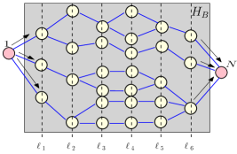
Figure 8: (Color online) A complex network topology that can be engineered for perfect transport with the modified XY Hamiltonian. Collapsing the equivalent nodes along the lines $\ell_{2}-\ell_{5}$ leads to three equivalent paths that can be suitably engineered for perfect transport.

V Conclusions and Outlook

Experimental implementation of quantum information transport requires relaxing many of the assumptions made in ideal schemes. In this paper we analyzed a physical situation that is closer to experimental settings – information transport in mixed-state spin networks with complex topologies. We first derived general conditions on propagators that allow perfect transport in these mixed-state spin networks. We used the conditions on the propagators to show that there exist classes of symmetry transformations on the Hamiltonians driving the transport for which the transport fidelity is invariant. We also showed that the propagator conditions also imply that transporting some mixed states requires fewer control requirements than pure state transport, an added advantage to using mixed-state channels in quantum information architectures.

In order to study quantum transfer in complex spin networks, we described the dynamics as a continuous quantum walk over the possible paths offered by the network. This description provided a graphical construction to predict the system evolution, which highlighted the need of correlating the transport processes occurring along different paths of the network to obtain perfect transport. We thus introduced a modified XY-Hamiltonian, based on Jordan-Wigner fermionization, that achieves correlation among paths by establishing a metric for the quantum walks occurring on the network. Conversely, the graphical construction could be as well used to study the generation from the usual XY-Hamiltonian of states of interest in measurement-based quantum computation Raussendorf et al. (2003).

Finally, the quantum-walk picture and the graphical construction lead us to define a constructive method to build complex networks from simpler ones, with appropriate coupling geometries and strengths, that achieve perfect transport. We thus found that there is considerable freedom in the choice of topology and interaction strength that still allows perfect transport in complex networks. While the requirement of a well-defined network topology could be further relaxed Ajoy and Cappellaro , the precise construction proposed in this paper would provide faster transport and the freedom in the coupling distributions could make these networks implementable in experimental systems.

Appendix A Constructing perfect transport unitaries

Here we show how the conditions specified in Eq. (10) could be used to construct perfect transport propagators. Our motivation for this is to demonstrate that the conditions of Eq. (10) are very weak, in the sense that is possible to construct an infinite classes of unitaries that support $Z_{1}\rightarrow Z_{N}$ transport.

Consider the matrix forms of $\hat{P}_{Z_{1}Z_{N}}^{\cal G}$ and $\hat{P}_{Z_{1}Z_{N}}^{\widetilde{\cal G}}$ in the two-dimensional $\{1,N\}$ subspace of ${\cal G}$ and $\widetilde{\cal G}$:

$${\cal G}\! \!\sim\! \!\Big{\{}\{\openone,Z_{1}Z_{N}\},\{Z_{1},Z_{N}\},\{X_{1},Y_{1}Z_{N}\},\{Y_{1},X_{1}Z_{N}\}\Big{\}}$$

$$\widetilde{\cal G}\! \!\sim\! \!\Big{\{}\{X_{1}X_{N},Y_{1}Y_{N}\},\{X_{1}Y_{N},Y_{1}X_{N}\},\{X_{N},Z_{1}Y_{N}\},$$ (29)

$$\{Y_{N},Z_{1}X_{N}\}\Big{\}}$$

where the $\sim$ refers to the restriction in the $\{1,N\}$ subspace. Then, for this order of basis, the matrix forms are block diagonal

$$\hat{P}_{Z_{1}Z_{N}}^{\cal G} = \textrm{diag}([X,X,-Y,Y])$$

$$\hat{P}_{Z_{1}Z_{N}}^{\widetilde{\cal G}} = \textrm{diag}([-X,X,-Y,Y])$$ (30)

where $X$ and $Y$ are the standard Pauli matrices, whose eigenvectors with eigenvalues $\pm 1$ are respectively $[1,\pm 1]^{T}$ and $[1,\pm i]^{T}$; this imposes a restriction on $U$. If $B_{\rm bulk},B_{\rm bulk}^{{}^{\prime}}\in{\rm span}\{\bf{B}_{\rm bulk}\}$, one can explicitly list from Eq. (10) possible forms of $U$ for perfect transport,

$$U_{1} = B_{\rm bulk}(\openone\pm Z_{1}Z_{N})+B_{\rm bulk}^{{}^{\prime}}(X_{1}X_{N}\pm Y_{1}Y_{N}),$$

$$U_{2} = B_{\rm bulk}(\openone\pm Z_{1}Z_{N})+B_{\rm bulk}^{{}^{\prime}}(X_{1}Y_{N}\mp Y_{1}X_{N}),$$

$$U_{3} = B_{\rm bulk}(Z_{1}\pm\openone Z_{N})+B_{\rm bulk}^{{}^{\prime}}(X_{1}X_{N}\pm Y_{1}Y_{N}),$$

$$U_{4} = B_{\rm bulk}(Z_{1}\pm Z_{N})+B_{\rm bulk}^{{}^{\prime}}(X_{1}Y_{N}\mp Y_{1}X_{N}),$$

$$U_{5} = B_{\rm bulk}(X_{1}\pm iY_{1}Z_{N})+B_{\rm bulk}^{{}^{\prime}}(X_{N}\mp iZ_{1}Y_{N}),$$

$$U_{6} = B_{\rm bulk}(X_{1}\pm iY_{1}Z_{N})+B_{\rm bulk}^{{}^{\prime}}(Y_{N}\pm iZ_{1}X_{N}),$$

$$U_{7} = B_{\rm bulk}(Y_{1}\pm iX_{1}Z_{N})+B_{\rm bulk}^{{}^{\prime}}(X_{N}\pm iZ_{1}Y_{N}),$$

$$U_{8} = B_{\rm bulk}(Y_{1}\pm iX_{1}Z_{N})+B_{\rm bulk}^{{}^{\prime}}(Y_{N}\mp iZ_{1}X_{N}),$$

Note that the bulk of the network specified by $B_{\rm bulk}$ and $B_{\rm bulk}^{{}^{\prime}}$ can be any arbitrary operators with equal norms. In fact, the invariance described in Sec. III.2 could be used to show that the eight forms of $U$ in Eq. (LABEL:eqn:A1.1) are equivalent to $U_{1}$ or $U_{2}$.

Of course, one can combine the forms in Eq. (LABEL:eqn:A1.1) to form other propagators that continue to support perfect transport. Consider for example a propagator constructed out of $U_{1}$ and $U_{2}$ in Eq. (LABEL:eqn:A1.1), with $B_{\rm bulk},B_{\rm bulk}^{{}^{\prime}}=\openone$

$$U=\lambda_{1}(1\pm Z_{1}Z_{N})+\lambda_{2}(X_{1}X_{N}\pm Y_{1}Y_{N})+\lambda_{3}(X_{1}Y_{N}\mp Y_{1}X_{N})$$

where $\lambda_{j}$ are coefficients to be determined. Then, from Eq. (4) we have

$$\langle{U}|{U}\rangle=1 \Rightarrow |\lambda_{1}|^{2}+|\lambda_{2}|^{2}+|\lambda_{3}|^{2}=1$$

$$\left\langle{U}\right|\hat{P}_{Z_{1}Z_{N}}\left|{U}\right\rangle=0 \Rightarrow |\lambda_{1}|^{2}=|\lambda_{2}|^{2}+|\lambda_{3}|^{2}$$

$$\left\langle{U}\right|\hat{P}_{Z_{N}}\left|{U}\right\rangle=0 \Rightarrow {\rm Im}(\lambda_{2}^{\ast}\lambda_{3})=0$$ (32)

Other conditions in Eq. (4) are satisifed trivially. Eq. (32) can be solved exactly; for example $\lambda_{j}=\{1/\sqrt{2},1/2,1/2\}$ is a solution. Importantly however, if the $B_{\rm bulk}^{{}^{\prime}}$’s were different from each other for $U_{1}$ and $U_{2}$, the set of equations Eq. (32) becomes far simpler.

In summary, achieving $Z_{1}\rightarrow Z_{N}$ transport requires weak conditions on the propagator driving the transport. This is as opposed to perfect pure state transport, that requires the propagators to be isomorphic to permutation operators Kostak et al. (2007) that are mirror symmetric Karbach and Stolze (2005) about the end spins of the network.

Appendix B Properties of flip-flop and double-quantum Hamiltonians

In this appendix, we present simple relations satisfied by the flip-flop (XY) operators that will be used in the main paper. Note that the double-quantum (DQ) operators in Eq. (14) follow analogous equations. In what follows, distinct indices label distinct positions on the spin network unless otherwise specified. We start with the definition of the operators $S$ and $E$:

$$E_{j}^{\pm}=\frac{1}{2}(\openone\pm Z_{j})\>,\qquad S_{j}^{\pm}=\frac{1}{2}(X_{j}\pm iY_{j}).$$ (33)

These operators satisfy the following product rules:

$$\begin{array}[]{l}Z_{j}S_{j}^{\pm}\!=\!\pm S_{j}^{\pm},\quad(S_{j}^{\pm})^{2}\!=\!E_{j}^{\pm}E_{j}^{\mp}=0,\\ S_{j}^{\pm}S_{j}^{\mp}\!=\!(E_{j}^{\pm})^{2}=E_{j}^{\pm}.\end{array}$$ (34)

We define the flip-flop operators $T_{ij}^{\pm}$ and $L_{ij}^{\pm}$:

$$T_{ij}^{\pm}=(S_{i}^{+}S_{j}^{-}\pm S_{i}^{-}S_{j}^{+});\quad L_{ij}^{\pm}=(E_{i}^{+}E_{j}^{-}\pm E_{i}^{-}E_{j}^{+})$$ (35)

From the definition in Eq. (35) it follows that

$$T_{ij}^{\pm}=\pm T_{ji}^{\pm}\>;\>Z_{j}T_{ij}^{+}=T_{ij}^{-}.$$

We have then the following product relations:

$$\begin{array}[]{l}\left(T_{ij}^{\pm}\right)^{2}=\pm L_{ij}^{+}\,,\quad T_{ij}^{\pm}L_{ij}^{+}=L_{ij}^{\pm}T_{ij}^{+}=T_{ij}^{\pm},\\ \left(L_{ij}^{\pm}\right)^{2}=L_{ij}^{+}\,,\quad T_{ij}^{\pm}T_{jk}^{+}=\frac{1}{2}\left(T_{ik}^{\pm}-Z_{j}T_{ik}^{\mp}\right)\end{array}$$ (36)

and the commutation relations:

$$\begin{array}[]{ll}\left[T_{ij}^{+},T_{jk}^{+}\right]=-Z_{j}T_{ik}^{-}\,,&\left[T_{ij}^{+},Z_{j}T_{ik}^{+}\right]=T_{kj}^{-},\\ \left[T_{ij}^{+},Z_{i}\right]=-2T_{ij}^{-}\,,&\left[T_{ij}^{-},Z_{i}\right]=-2T_{ij}^{+}.\end{array}$$ (37)

We define the modified flip-flop operators $\widetilde{T}_{ij}^{\pm}$,

$$\widetilde{T}_{ij}^{\pm}=T_{ij}^{\pm}\prod_{i<u<j}Z_{u},$$ (38)

obtained by multiplying the flip-flop operator in Eq. (35) by a factor of $Z_{u}$ for all nodes between $i$ and $j$. The modified flip-flop operators follow especially simple commutation rules

$$\left[\widetilde{T}_{ij}^{+},\widetilde{T}_{jk}^{\pm}\right]=-\widetilde{T}_{ik}^{\mp}\>;\>\left[\widetilde{T}_{ij}^{+},\widetilde{T}_{k\ell}^{\pm}\right]=0$$ (39)

Note that crucially, these commutators only depend on the initial and final nodes ($i$ and $k$), and are independent of intermediate nodes. In a physical analogy, the modified operators $\widetilde{T}_{ij}^{+}$ behave as if they were path independent. Thus, when considering two (or more) paths, we could omit any intermediate node, since it would not enter in the ensuing commutators. We then denote equivalent nodes in parenthesis –for example, $(j,k)$ means nodes $j$ and $k$ are equivalent– and define the collapsed operators:

$$\widetilde{T}_{i(j,k)}^{\pm}=\frac{1}{\sqrt{\gamma_{ij}^{2}+\gamma_{ik}^{2}}}\left(\gamma_{ij}\widetilde{T}_{ij}^{\pm}+\gamma_{ik}\widetilde{T}_{ik}^{\pm}\right),$$ (40)

where $\gamma_{ij},\ \gamma_{ik}$ are arbitrary parameters, $0\!<\!\gamma_{ij},\!\gamma_{ik}\!<~{}\!1$. The collapsed operators satisfy commutation relations similar to Eq. (39):

$$\begin{array}[]{l}\left[\widetilde{T}_{i(j,k)}^{+},\widetilde{T}_{(j,k)\ell}^{\pm}\right]\!=\!-\widetilde{T}_{i\ell}^{\mp}\,,\ \ \left[\widetilde{T}_{(j,k)i}^{+},\widetilde{T}_{i\ell}^{\pm}\right]\!=\!-\widetilde{T}_{(j,k)\ell}^{\mp},\\ \displaystyle\left[\widetilde{T}_{(j,k)i}^{+},\widetilde{T}_{i(m,n)}^{\pm}\right]=-\widetilde{T}_{(j,k)(m,n)}^{\mp}\end{array}$$ (41)

The collapsed operators in Eq. (40) can be generalized. If $\mathbf{I}=(a_{1},a_{2},\cdots,a_{m})$ and ${\bf J}=(b_{1},b_{2},\cdots,b_{n})$ denote two sets of equivalent nodes, we have the collapsed operator

$$\widetilde{T}_{{\bf IJ}}^{\pm}=\frac{1}{\sqrt{\sum_{i=1}^{m}\sum_{j=1}^{n}\gamma_{a_{i}b_{j}}^{2}}}\sum_{i=1}^{m}\sum_{j=1}^{n}\gamma_{a_{i}b_{j}}\widetilde{T}_{a_{i}b_{j}}^{\pm}\>,$$ (42)

which satisfies the commutation relationships:

$$\left[\widetilde{T}_{\mathbf{IJ}}^{+},\widetilde{T}_{\mathbf{JK}}^{\pm}\right]=-\widetilde{T}_{\mathbf{IK}}^{\mp}\>;\>\left[\widetilde{T}_{\mathbf{IJ}}^{+},\widetilde{T}_{\mathbf{KL}}^{\pm}\right]=0.$$ (43)

References

- Ladd et al. (2010) T. D. Ladd, F. Jelezko, R. Laflamme, Y. Nakamura, C. Monroe, and J. L. O’Brien, Nature 464, 45 (2010).
- Cirac et al. (1999) J. I. Cirac, A. K. Ekert, S. F. Huelga, and C. Macchiavello, Phys. Rev. A 59, 4249 (1999).
- Oi et al. (2006) D. K. L. Oi, S. J. Devitt, and L. C. L. Hollenberg, Phys. Rev. A 74, 052313 (2006).
- Jiang et al. (2007) L. Jiang, J. M. Taylor, A. S. Sorensen, and M. D. Lukin, Phys. Rev. A 76, 062323 (2007).
- Kimble (2008) H. J. Kimble, Nature 453, 1023 (2008).
- Meter et al. (2008) R. V. Meter, W. J. Munro, K. Nemoto, and K. M. Itoh, J. Emerg. Technol. Comput. Syst. 3, 2:1 (2008).
- Bose (2003) S. Bose, Phys. Rev. Lett. 91, 207901 (2003).
- Kay (2010) A. Kay, Int. J. of Quantum Info. 8, 641 (2010).
- Christandl et al. (2004) M. Christandl, N. Datta, A. Ekert, and A. J. Landahl, Phys. Rev. Lett. 92, 187902 (2004).
- Albanese et al. (2004) C. Albanese, M. Christandl, N. Datta, and A. Ekert, Phys. Rev. Lett. 93, 230502 (2004).
- Nikolopoulos et al. (2004a) G. M. Nikolopoulos, D. Petrosyan, and P. Lambropoulos, J. Phys.: Cond. Matt. 16, 4991 (2004a).
- Nikolopoulos et al. (2004b) G. M. Nikolopoulos, D. Petrosyan, and P. Lambropoulos, Europhys. Lett. 65, 297 (2004b).
- Gualdi et al. (2008) G. Gualdi, V. Kostak, I. Marzoli, and P. Tombesi, Phys. Rev. A 78, 022325 (2008).
- Wojcik et al. (2005) A. Wojcik, T. Luczak, P. Kurzynski, A. Grudka, T. Gdala, and M. Bednarska, Phys. Rev. A 72, 034303 (2005).
- Li et al. (2005) Y. Li, T. Shi, B. Chen, Z. Song, and C.-P. Sun, Phys. Rev. A 71, 022301 (2005).
- Wang et al. (2011) Y. Wang, F. Shuang, and H. Rabitz, Phys. Rev. A 84, 012307 (2011).
- Burgarth and Bose (2005) D. Burgarth and S. Bose, Phys. Rev. A 71, 052315 (2005).
- Álvarez et al. (2010) G. A. Álvarez, M. Mishkovsky, E. P. Danieli, P. R. Levstein, H. M. Pastawski, and L. Frydman, Phys. Rev. A 81, 060302 (2010).
- Fitzsimons and Twamley (2006) J. Fitzsimons and J. Twamley, Phys. Rev. Lett. 97, 090502 (2006).
- Burgarth et al. (2007) D. Burgarth, V. Giovannetti, and S. Bose, Phys. Rev. A 75, 062327 (2007).
- Caneva et al. (2009) T. Caneva, M. Murphy, T. Calarco, R. Fazio, S. Montangero, V. Giovannetti, and G. E. Santoro, Phys. Rev. Lett. 103, 240501 (2009).
- Burgarth et al. (2010) D. Burgarth, K. Maruyama, M. Murphy, S. Montangero, T. Calarco, F. Nori, and M. B. Plenio, Phys. Rev. A 81, 040303 (2010).
- Cappellaro et al. (2007) P. Cappellaro, C. Ramanathan, and D. G. Cory, Phys. Rev. Lett. 99, 250506 (2007).
- DiFranco et al. (2008) C. DiFranco, M. Paternostro, and M. S. Kim, Phys. Rev. Lett. 101, 230502 (2008).
- Cappellaro et al. (2011) P. Cappellaro, L. Viola, and C. Ramanathan, Phys. Rev. A 83, 032304 (2011).
- Yao et al. (2011) N. Y. Yao, L. Jiang, A. V. Gorshkov, Z.-X. Gong, A. Zhai, L.-M. Duan, and M. D. Lukin, Phys. Rev. Lett. 106, 040505 (2011).
- Kaur and Cappellaro (2011) G. Kaur and P. Cappellaro, ArXiv e-prints (2011), arXiv:1112.0459 [quant-ph] .
- Panitchayangkoon et al. (2011) G. Panitchayangkoon, D. V. Voronine, D. Abramavicius, J. R. Caram, N. H. C. Lewis, S. Mukamel, and G. S. Engel, Proc. Nat. Acad. Sc. 108, 20908 (2011).
- Engel et al. (2007) G. S. Engel, T. R. Calhoun, E. L. Read, T.-K. Ahn, T. Mancal, Y.-C. Cheng, R. E. Blankenship, and G. R. Fleming, Nature 446, 782 (2007).
- Mohseni et al. (2008) M. Mohseni, P. Rebentrost, S. Lloyd, and A. Aspuru-Guzik, J. Chem. Phys. 129, 174106 (2008).
- Kostak et al. (2007) V. Kostak, G. M. Nikolopoulos, and I. Jex, Phys. Rev. A 75, 042319 (2007).
- Aharonov et al. (1993) Y. Aharonov, L. Davidovich, and N. Zagury, Phys. Rev. A 48, 1687–1690 (1993).
- Baum et al. (1985) J. Baum, M. Munowitz, A. N. Garroway, and A. Pines, J. Chem. Phys. 83, 2015 (1985).
- Munowitz et al. (1987) M. Munowitz, A. Pines, and M. Mehring, J. Chem. Phys. 86, 3172 (1987).
- Mülken and Blumen (2011) O. Mülken and A. Blumen, Physics Reports 502, 37 (2011).
- Feder (2006) D. L. Feder, Phys. Rev. Lett. 97, 180502 (2006).
- Krovi and Brun (2007) H. Krovi and T. A. Brun, Phys. Rev. A 75, 062332 (2007).
- Bernasconi et al. (2008) A. Bernasconi, C. Godsil, and S. Severini, Phys. Rev. A 78, 052320 (2008).
- Pemberton-Ross and Kay (2011) P. J. Pemberton-Ross and A. Kay, Phys. Rev. Lett. 106, 020503 (2011).
- Osborne and Linden (2004) T. J. Osborne and N. Linden, Phys. Rev. A 69, 052315 (2004).
- Yung (2006) M.-H. Yung, Phys. Rev. A 74, 030303 (2006).
- Cho et al. (2005) H. J. Cho, T. D. Ladd, J. Baugh, D. G. Cory, and C. Ramanathan, Phys. Rev. B 72, 054427 (2005).
- Sorensen et al. (1984) O. Sorensen, G. Eich, M. Levitt, G. Bodenhausen, and R. Ernst, Progress in Nuclear Magnetic Resonance Spectroscopy 16, 163 (1984).
- Ajoy et al. (2012) A. Ajoy, R. K. Rao, A. Kumar, and P. Rungta, Phys. Rev. A 85, 030303 (2012).
- Karbach and Stolze (2005) P. Karbach and J. Stolze, Phys. Rev. A 72, 030301 (2005).
- Kay (2011) A. Kay, Phys. Rev. A 84, 022337 (2011).
- Hincks et al. (2011) I. N. Hincks, D. G. Cory, and C. Ramanathan, ArXiv e-prints (2011), arXiv:1111.0944 [quant-ph] .
- Markiewicz and Wiesniak (2009) M. Markiewicz and M. Wiesniak, Phys. Rev. A 79, 054304 (2009).
- Benjamin and Bose (2003) S. C. Benjamin and S. Bose, Phys. Rev. Lett. 90, 247901 (2003).
- Clark et al. (2005) S. R. Clark, C. M. Alves, and D. Jaksch, New J. Phys. 7, 124 (2005).
- Di Franco et al. (2007) C. Di Franco, M. Paternostro, G. M. Palma, and M. S. Kim, Phys. Rev. A 76, 042316 (2007).
- Clark et al. (2007) S. R. Clark, A. Klein, M. Bruderer, and D. Jaksch, New J. Phys. 9, 202 (2007).
- Di Franco et al. (2009) C. Di Franco, M. Paternostro, and M. S. Kim, Phys. Rev. Lett. 102, 187203 (2009).
- Terhal and DiVincenzo (2002) B. M. Terhal and D. P. DiVincenzo, Phys. Rev. A 65, 032325 (2002).
- Barthel et al. (2009) T. Barthel, C. Pineda, and J. Eisert, Phys. Rev. A 80, 042333 (2009).
- Jordan and Wigner (1928) P. Jordan and E. Wigner, Z. Phys. B 47, 631 (1928).
- Lieb et al. (1961) E. Lieb, T. Schultz, and D. Mattis, Annals of Physics 16, 407 (1961).
- Childs (2009) A. M. Childs, Phys. Rev. Lett. 102, 180501 (2009).
- Raussendorf et al. (2003) R. Raussendorf, D. E. Browne, and H. J. Briegel, Phys. Rev. A 68, 022312 (2003).
- (60) A. Ajoy and P. Cappellaro, “Perfect quantum state transport in arbitrary spin networks,” Unpublished.