On the Spin of the X(3872)𝑋3872X(3872)

R. Faccini, F. Piccinini, A. Pilloni and A.D. Polosa Dipartimento di Fisica and INFN, ‘Sapienza’ Università di Roma,
Piazzale A. Moro 2, Roma, I-00185, Italy     
INFN Pavia, Via A. Bassi 6, Pavia, I-27100, Italy
Abstract

Whether the much studied X(3872)𝑋3872X(3872) is an axial or tensor resonance makes an important difference to its interpretation. A recent paper by the BaBar collaboration delAmoSanchez:2010jr raised the viable hypothesis that it might be a JPC=2+superscript𝐽𝑃𝐶superscript2absentJ^{PC}=2^{-+} state based on the π+ππ0superscript𝜋superscript𝜋superscript𝜋0\pi^{+}\pi^{-}\pi^{0} spectrum in the XJ/ψω𝑋𝐽𝜓𝜔X\to J/\psi\;\omega decays. Furthermore, the Belle collaboration published the π+πsuperscript𝜋superscript𝜋\pi^{+}\pi^{-} invariant mass and spin-sensitive angular distributions in XJ/ψρ𝑋𝐽𝜓𝜌X\to J/\psi\;\rho decays Choi:2011fc .

Starting from a general parametrization of the decay amplitudes for the axial and tensor quantum numbers of the X𝑋X, we re-analyze the whole set of available data. The level of agreement of the two spin hypotheses with data is interpreted with a rigorous statistical approach based on Monte Carlo simulations in order to be able to combine all the distributions regardless of their different levels of sensitivity to the spin of the X𝑋X.

Our analysis returns a probability of 5.5% and 0.1% for the agreement with data of the 1++superscript1absent1^{++} and 2+superscript2absent2^{-+} hypotheses, respectively, once we combine the whole information (angular and mass distributions) from both channels. On the other hand, the separate analysis of J/ψρ𝐽𝜓𝜌J/\psi\;\rho (angular and mass distributions) and J/ψω𝐽𝜓𝜔J/\psi\;\omega (mass distribution) indicates that the 2+superscript2absent2^{-+} assignment is excluded at the 99.9% C.L. by the former case, while the latter excludes at the same level the 1++superscript1absent1^{++} hypothesis. There are therefore indications that the two decay modes behave in a different way.

PACS: 13.25.Ft, 14.40.Rt

I Introduction

Although the X(3872)𝑋3872X(3872) resonance is the most studied among the exotic XYZ𝑋𝑌𝑍XYZ states, since its discovery in 2003, its quantum numbers have not been definitively identified yet.

The CDF collaboration concluded from the analysis of the angular distributions and correlations of the X𝑋X decay products that the possible quantum numbers are JPC=1++superscript𝐽𝑃𝐶superscript1absentJ^{PC}=1^{++} or 2+superscript2absent2^{-+} Abulencia:2006ma . Similar results have been found very recently by the BELLE collaboration Choi:2011fc . In the latter paper the π+πsuperscript𝜋superscript𝜋\pi^{+}\pi^{-} invariant mass distribution is analyzed under the 1++superscript1absent1^{++} and 2+superscript2absent2^{-+} hypotheses, finding preference for the former whereas no preferred assignment emerges if an interfering contribution with the isospin-violating decay ωπ+π𝜔superscript𝜋superscript𝜋\omega\to\pi^{+}\pi^{-} is added to the amplitude.

The picture becomes more puzzling as one considers the analysis by the BaBar Collaboration of the decay XJ/ψπ+ππ0𝑋𝐽𝜓superscript𝜋superscript𝜋superscript𝜋0X\to J/\psi\;\pi^{+}\pi^{-}\pi^{0} delAmoSanchez:2010jr . The expected 3π3𝜋3\pi invariant mass distribution agrees with data slightly better if the 2+superscript2absent2^{-+} signature is assumed. This result on the 3π3𝜋3\pi spectrum was later confirmed in Brazzi:2011fq .

In a recent paper Hanhart:2011tn the pion invariant masses in the decays XJ/ψ 2π𝑋𝐽𝜓2𝜋X\to J/\psi\;2\pi and XJ/ψ 3π𝑋𝐽𝜓3𝜋X\to J/\psi\;3\pi are simultaneously analyzed with a combined fit, concluding that present data favor the 1++superscript1absent1^{++} assignment. In our view, the 2π2𝜋2\pi invariant mass distribution is not able to resolve the two hypotheses despite of the high statistics, and the way the fit was performed leads to the dilution of the sensitivity of the 3π3𝜋3\pi channel.

To improve the analysis of all available data sensitive to the spin of the X𝑋X i)i) we write the decay matrix elements for both the 1++superscript1absent1^{++} and 2+superscript2absent2^{-+} hypotheses as given by enforcing Lorentz invariance and parity considerations, ii)ii) we give a functional dependency on the decay momenta to the couplings introducing a length scale R𝑅R – which is to be related to the finite size of the hadrons participating to the interactions, iii)iii) we use the matrix elements of ρ𝜌\rho and ω𝜔\omega decays to take into account the appropriate decay waves; we do not pursue the Blatt-Weisskopf description as we find that all spin structure can appropriately be taken into account with no further approximations, iv)iv) we perform a global fit to exploit the information contained in all the distributions available and we adopt a statistical approach appropriate when distributions with different sensitivities to the parameters of interest are combined.

II Matrix elements

The matrix elements describing the amplitudes XJ/ψV𝑋𝐽𝜓𝑉X\to J/\psi\,V (where V=ρ,ω𝑉𝜌𝜔V=\rho,\omega) are obtained by Lorentz, gauge invariance and parity considerations leading to the formulae reported below Brazzi:2011fq .

In the X(1++)𝑋superscript1absentX(1^{++}) case we have

ψ(ϵ,p)V(η,q)|X(λ,P)=g1ψVϵμνρσλμ(P)ϵν(p)ηρ(q)Pσinner-product𝜓italic-ϵ𝑝𝑉𝜂𝑞𝑋𝜆𝑃subscript𝑔1𝜓𝑉superscriptitalic-ϵ𝜇𝜈𝜌𝜎subscript𝜆𝜇𝑃subscriptsuperscriptitalic-ϵ𝜈𝑝subscriptsuperscript𝜂𝜌𝑞subscript𝑃𝜎\langle\psi(\epsilon,p)V(\eta,q)|X(\lambda,P)\rangle=g_{1\psi V}\;\epsilon^{\mu\nu\rho\sigma}\;\lambda_{\mu}(P)\;\epsilon^{*}_{\nu}(p)\;\eta^{*}_{\rho}(q)\;P_{\sigma} (1)

the polarization vectors carry a complex conjugation when referred to final states.

In the 2+superscript2absent2^{-+} case we have a more complicated structure

ψ(ϵ,p)V(η,q)|X(π,P)=g2ψVTA+g2ψVTBinner-product𝜓italic-ϵ𝑝𝑉𝜂𝑞𝑋𝜋𝑃subscript𝑔2𝜓𝑉subscript𝑇𝐴superscriptsubscript𝑔2𝜓𝑉subscript𝑇𝐵\langle\psi(\epsilon,p)V(\eta,q)|X(\pi,P)\rangle=g_{2\psi V}\;T_{A}+g_{2\psi V}^{\prime}\;T_{B} (2)

where π𝜋\pi is the polarization tensor for a spin two particle with mass111 The sum over polarizations is polπμν(k)παβ(k)=12TμαTνβ+12TμβTνα13TμνTαβsubscriptpolsubscript𝜋𝜇𝜈𝑘subscriptsuperscript𝜋𝛼𝛽𝑘12subscript𝑇𝜇𝛼subscript𝑇𝜈𝛽12subscript𝑇𝜇𝛽subscript𝑇𝜈𝛼13subscript𝑇𝜇𝜈subscript𝑇𝛼𝛽\sum_{\rm pol}\pi_{\mu\nu}(k)\pi^{*}_{\alpha\beta}(k)=\frac{1}{2}T_{\mu\alpha}T_{\nu\beta}+\frac{1}{2}T_{\mu\beta}T_{\nu\alpha}-\frac{1}{3}T_{\mu\nu}T_{\alpha\beta} (3) with Tμν=gμν+kμkν/m2subscript𝑇𝜇𝜈subscript𝑔𝜇𝜈subscript𝑘𝜇subscript𝑘𝜈superscript𝑚2T_{\mu\nu}=-g_{\mu\nu}+k_{\mu}k_{\nu}/m^{2} and k2=m2superscript𝑘2superscript𝑚2k^{2}=m^{2}. and a standard notation is used for the remaining polarization vectors. We find that TAsubscript𝑇𝐴T_{A} and TBsubscript𝑇𝐵T_{B} are given by

TA=ϵα(p)παμ(P)ϵμνρσpνqρησ(q)(ϵ,pη,q)T_{A}=\epsilon^{*\alpha}(p)\>\pi_{\alpha\mu}(P)\;\epsilon^{\mu\nu\rho\sigma}\;p_{\nu}\;q_{\rho}\;\eta^{*}_{\sigma}(q)-(\epsilon,p\leftrightarrow\eta,q) (4)

and

TB=Qαπαμ(P)ϵμνρσPνϵρ(p)ησ(q)subscript𝑇𝐵superscript𝑄𝛼subscript𝜋𝛼𝜇𝑃superscriptitalic-ϵ𝜇𝜈𝜌𝜎subscript𝑃𝜈subscriptsuperscriptitalic-ϵ𝜌𝑝subscriptsuperscript𝜂𝜎𝑞T_{B}=Q^{\alpha}\>\pi_{\alpha\mu}(P)\;\epsilon^{\mu\nu\rho\sigma}\;P_{\nu}\;\epsilon^{*}_{\rho}(p)\;\eta^{*}_{\sigma}(q) (5)

where Q=pq𝑄𝑝𝑞Q=p-q and P=p+q𝑃𝑝𝑞P=p+q.

The coupling g1ψVsubscript𝑔1𝜓𝑉g_{1\psi V} is real whereas the couplings g2ψVsubscript𝑔2𝜓𝑉g_{2\psi V} and g2ψVsuperscriptsubscript𝑔2𝜓𝑉g_{2\psi V}^{\prime} are separately real but can have a complex relative phase. This is due to the fact that, on the basis of Lorentz invariance and parity conservation, we can indeed write three terms TA(λ),TB(λ)superscriptsubscript𝑇𝐴𝜆superscriptsubscript𝑇𝐵𝜆T_{A}^{(\lambda)},T_{B}^{(\lambda)} and TC(λ)superscriptsubscript𝑇𝐶𝜆T_{C}^{(\lambda)} where λ𝜆\lambda labels one out of the 3×3×53353\times 3\times 5 polarization combinations which define TA,TB,TCsubscript𝑇𝐴subscript𝑇𝐵subscript𝑇𝐶T_{A},T_{B},T_{C}. TCsubscript𝑇𝐶T_{C} is the same as TAsubscript𝑇𝐴T_{A} but with a plus relative sign between the two terms on the rhs of (4). Only two out of these three terms are linearly independent (say TAsubscript𝑇𝐴T_{A} and TBsubscript𝑇𝐵T_{B}) for

|λ=13×3×5TA(λ)TC(λ)|2=λ|TA(λ)|2λ|TC(λ)|2superscriptsuperscriptsubscript𝜆1335superscriptsubscript𝑇𝐴𝜆superscriptsubscript𝑇𝐶𝜆2subscript𝜆superscriptsuperscriptsubscript𝑇𝐴𝜆2subscript𝜆superscriptsuperscriptsubscript𝑇𝐶𝜆2\left|\sum_{\lambda=1}^{3\times 3\times 5}T_{A}^{(\lambda)}T_{C}^{(\lambda)*}\right|^{2}=\sum_{\lambda}|T_{A}^{(\lambda)}|^{2}\sum_{\lambda}|T_{C}^{(\lambda)}|^{2} (6)

which is the equality of the Schwartz inequality: this holds if z1TA=z2TCsubscript𝑧1subscript𝑇𝐴subscript𝑧2subscript𝑇𝐶z_{1}T_{A}=z_{2}T_{C} where z1subscript𝑧1z_{1} and z2subscript𝑧2z_{2} are two complex numbers both different from zero. Thus we can exclude TCsubscript𝑇𝐶T_{C} and retain TBsubscript𝑇𝐵T_{B} and, in general, z1TAsubscript𝑧1subscript𝑇𝐴z_{1}T_{A} to characterize the decay amplitude.

In Refs. Choi:2011fc ; delAmoSanchez:2010jr ; Hanhart:2011tn the P𝑃P-wave fit functions contain a Blatt-Weisskopf angular momentum barrier factor of the form (1+R2q2)1/2superscript1superscript𝑅2superscript𝑞absent212\left(1+R^{2}q^{*2}\right)^{-1/2}, where qsuperscript𝑞q^{*} is the X𝑋X decay 3-momentum. The value of R𝑅R cannot be extracted from data since the P𝑃P-wave distribution will approach the S𝑆S-wave distribution in the limit R𝑅R\to\infty, so that if we let R𝑅R free, the fit will not converge. On the other hand, in our discussion we do not need any barrier factor the decay wave being dictated by the expressions of the matrix elements. We instead take into account the finite size of the X𝑋X (and of V𝑉V and J/ψ𝐽𝜓J/\psi as well) introducing a ‘polar’ form factor, namely

gg(1+R2q2)n𝑔𝑔superscript1superscript𝑅2superscript𝑞absent2𝑛g\to\frac{g}{(1+R^{2}q^{*2})^{n}} (7)

where g𝑔g stands in general for g1ψVsubscript𝑔1𝜓𝑉g_{1\psi V}, g2ψVsubscript𝑔2𝜓𝑉g_{2\psi V} and g2ψVsuperscriptsubscript𝑔2𝜓𝑉g_{2\psi V}^{\prime}. We tested the values n=1𝑛1n=1 and n=2𝑛2n=2 (the latter coinciding with the Fourier transform of a an exponential g(r)exp(r/R)similar-to𝑔𝑟𝑟𝑅g(r)\sim\exp(-r/R) strong charge distribution). Both the fitting functions turn out to be rather effective at improving our results, with no significative change for the the two choices of n𝑛n. We also underscore that g1ψVsubscript𝑔1𝜓𝑉g_{1\psi V} (regulating the S𝑆S-wave decay) is assumed to have the same polar behavior since Eq. (7) does not concern any orbital angular momentum considerations. The size parameters RJsubscript𝑅𝐽R_{J} will eventually be fitted from data.

As for the ρ𝜌\rho and ω𝜔\omega decay amplitudes, we use

π+(p)π(q)|ρ(ϵ,P)=gρ2πϵpinner-productsuperscript𝜋𝑝superscript𝜋𝑞𝜌italic-ϵ𝑃subscript𝑔𝜌2𝜋italic-ϵ𝑝\langle\pi^{+}(p)\pi^{-}(q)|\rho\left(\epsilon,P\right)\rangle=g_{\rho 2\pi}\,\epsilon\cdot p (8)

which describes a P𝑃P-wave decay (the square modulus of this matrix element is gρ2π2subscriptsuperscript𝑔2𝜌2𝜋g^{2}_{\rho 2\pi} times the decay momentum squared). For the ω𝜔\omega we have

π+(p)π(q)π0(r)|ω(ϵ,P)=gω3πϵμνρσϵμpνqρrσinner-productsuperscript𝜋𝑝superscript𝜋𝑞superscript𝜋0𝑟𝜔italic-ϵ𝑃subscript𝑔𝜔3𝜋superscriptitalic-ϵ𝜇𝜈𝜌𝜎subscriptitalic-ϵ𝜇subscript𝑝𝜈subscript𝑞𝜌subscript𝑟𝜎\langle\pi^{+}(p)\pi^{-}(q)\pi^{0}(r)|\omega\left(\epsilon,P\right)\rangle=g_{\omega 3\pi}\,\epsilon^{\mu\nu\rho\sigma}\epsilon_{\mu}p_{\nu}q_{\rho}r_{\sigma} (9)

The last two couplings will simply be written in terms of the partial widths Γ(ρ2π)Γ𝜌2𝜋\Gamma(\rho\to 2\pi) and Γ(ω3π)Γ𝜔3𝜋\Gamma(\omega\to 3\pi), as shown in the next section.

III Decay Widths

We have to calculate the partial widths Γ(XJ/ψπ+π)Γ𝑋𝐽𝜓superscript𝜋superscript𝜋\Gamma(X\to J/\psi\;\pi^{+}\pi^{-}) and Γ(XJ/ψπ+ππ0)Γ𝑋𝐽𝜓superscript𝜋superscript𝜋superscript𝜋0\Gamma(X\to J/\psi\;\pi^{+}\pi^{-}\pi^{0}). In what follows we will neglect the ρ𝜌\rho-ω𝜔\omega mixing since we demonstrate in Appendix A that it does not alter significantly the results.

The partial widths in the narrow width approximation are Brazzi:2011fq

Γ(XJ/ψπ+π)=12J+1148πmX2𝑑spol|ψρ(s)|X|2p(mX2,mψ2,s)×1π1(smρ2)2+(mρΓρ)2𝑑Φ(2)pol|π+π|ρ(s)|2Γ𝑋𝐽𝜓superscript𝜋superscript𝜋12𝐽1148𝜋subscriptsuperscript𝑚2𝑋differential-d𝑠subscriptpolsuperscriptinner-product𝜓𝜌𝑠𝑋2superscript𝑝subscriptsuperscript𝑚2𝑋subscriptsuperscript𝑚2𝜓𝑠1𝜋1superscript𝑠superscriptsubscript𝑚𝜌22superscriptsubscript𝑚𝜌subscriptΓ𝜌2differential-dsuperscriptΦ2subscriptpolsuperscriptinner-productsuperscript𝜋superscript𝜋𝜌𝑠2\begin{split}\Gamma(X\to J/\psi\;\pi^{+}\pi^{-})&=\frac{1}{2J+1}\frac{1}{48\pi m^{2}_{X}}\int\;ds\;\sum_{\begin{subarray}{c}{\rm pol}\end{subarray}}|\langle\psi\;\rho(s)|X\rangle|^{2}p^{*}(m^{2}_{X},m^{2}_{\psi},s)\\ &\quad\times\frac{1}{\pi}\frac{1}{(s-m_{\rho}^{2})^{2}+(m_{\rho}\Gamma_{\rho})^{2}}\int d\Phi^{(2)}\sum_{\begin{subarray}{c}{\rm pol}\end{subarray}}|\langle\pi^{+}\pi^{-}|\rho(s)\rangle|^{2}\end{split} (10)

where by dΦ(2)𝑑superscriptΦ2d\Phi^{(2)} we mean the 2-body phase space measure. The decay momentum qsuperscript𝑞q^{*} in the matrix element ψρ(s)|Xinner-product𝜓𝜌𝑠𝑋\langle\psi\;\rho(s)|X\rangle coincides with qp(mX2,mψ2,s)superscript𝑞superscript𝑝subscriptsuperscript𝑚2𝑋subscriptsuperscript𝑚2𝜓𝑠q^{*}\equiv p^{*}(m^{2}_{X},m^{2}_{\psi},s); similarly for the width in J/ψω𝐽𝜓𝜔J/\psi\;\omega discussed below.

The sum over polarizations in (8), simply yields

pol|π+π|ρ(s)|2=gρ2π2p(s,mπ2,mπ2)2subscriptpolsuperscriptinner-productsuperscript𝜋superscript𝜋𝜌𝑠2superscriptsubscript𝑔𝜌2𝜋2superscript𝑝superscript𝑠subscriptsuperscript𝑚2𝜋subscriptsuperscript𝑚2𝜋2\sum_{\begin{subarray}{c}{\rm pol}\end{subarray}}|\langle\pi^{+}\pi^{-}|\rho(s)\rangle|^{2}=g_{\rho 2\pi}^{2}\;p^{*}(s,m^{2}_{\pi},m^{2}_{\pi})^{2} (11)

Finally, we can eliminate the coupling by evaluating the (11) on the mass-shell and by relating it to the partial width Γ(ρππ)Γ𝜌𝜋𝜋\Gamma\left(\rho\to\pi\pi\right)

gρ2π2=6mρ2Γ(ρππ)4πp(mρ2,mπ2,mπ2)3subscriptsuperscript𝑔2𝜌2𝜋6subscriptsuperscript𝑚2𝜌Γ𝜌𝜋𝜋4𝜋superscript𝑝superscriptsuperscriptsubscript𝑚𝜌2subscriptsuperscript𝑚2𝜋subscriptsuperscript𝑚2𝜋3g^{2}_{\rho 2\pi}=6m^{2}_{\rho}\;\Gamma(\rho\to\pi\pi)\;\frac{4\pi}{p^{*}(m_{\rho}^{2},m^{2}_{\pi},m^{2}_{\pi})^{3}} (12)

Inserting the above expressions (11), (12) into (10) gives

Γ(XJ/ψπ+π)=12J+118πmX2𝑑spol|ψρ(s)|X|2p(mX2,mψ2,s)×1πmρΓρ(ρππ)(smρ2)2+(mρΓρ)2mρs(p(s,mπ2,mπ2)p(mρ2,mπ2,mπ2))3Γ𝑋𝐽𝜓superscript𝜋superscript𝜋12𝐽118𝜋subscriptsuperscript𝑚2𝑋differential-d𝑠subscriptpolsuperscriptinner-product𝜓𝜌𝑠𝑋2superscript𝑝subscriptsuperscript𝑚2𝑋subscriptsuperscript𝑚2𝜓𝑠1𝜋subscript𝑚𝜌subscriptΓ𝜌𝜌𝜋𝜋superscript𝑠superscriptsubscript𝑚𝜌22superscriptsubscript𝑚𝜌subscriptΓ𝜌2subscript𝑚𝜌𝑠superscriptsuperscript𝑝𝑠subscriptsuperscript𝑚2𝜋subscriptsuperscript𝑚2𝜋superscript𝑝superscriptsubscript𝑚𝜌2subscriptsuperscript𝑚2𝜋subscriptsuperscript𝑚2𝜋3\begin{split}\Gamma(X\to J/\psi\;\pi^{+}\pi^{-})&=\frac{1}{2J+1}\frac{1}{8\pi m^{2}_{X}}\int\;ds\;\sum_{\begin{subarray}{c}{\rm pol}\end{subarray}}|\langle\psi\;\rho(s)|X\rangle|^{2}p^{*}(m^{2}_{X},m^{2}_{\psi},s)\\ &\quad\times\frac{1}{\pi}\frac{m_{\rho}\Gamma_{\rho}\;\mathcal{BR}(\rho\to\pi\pi)}{(s-m_{\rho}^{2})^{2}+(m_{\rho}\Gamma_{\rho})^{2}}\frac{m_{\rho}}{\sqrt{s}}\left(\frac{p^{*}(s,m^{2}_{\pi},m^{2}_{\pi})}{p^{*}(m_{\rho}^{2},m^{2}_{\pi},m^{2}_{\pi})}\right)^{3}\\ \end{split} (13)

Similarly, for the ω𝜔\omega we obtain

Γ(XJ/ψπ+ππ0)=12J+1148πmX2𝑑spol|ψω(s)|X|2p(mX2,mψ2,s)×1π1(smω2)2+(mωΓω)2𝑑Φ(3)pol|π+ππ0|ω(s)|2Γ𝑋𝐽𝜓superscript𝜋superscript𝜋superscript𝜋012𝐽1148𝜋subscriptsuperscript𝑚2𝑋differential-d𝑠subscriptpolsuperscriptinner-product𝜓𝜔𝑠𝑋2superscript𝑝subscriptsuperscript𝑚2𝑋subscriptsuperscript𝑚2𝜓𝑠1𝜋1superscript𝑠superscriptsubscript𝑚𝜔22superscriptsubscript𝑚𝜔subscriptΓ𝜔2differential-dsuperscriptΦ3subscriptpolsuperscriptinner-productsuperscript𝜋superscript𝜋superscript𝜋0𝜔𝑠2\begin{split}\Gamma(X\to J/\psi\;\pi^{+}\pi^{-}\pi^{0})&=\frac{1}{2J+1}\frac{1}{48\pi m^{2}_{X}}\int\;ds\;\sum_{\begin{subarray}{c}{\rm pol}\end{subarray}}|\langle\psi\;\omega(s)|X\rangle|^{2}p^{*}(m^{2}_{X},m^{2}_{\psi},s)\\ &\quad\times\frac{1}{\pi}\frac{1}{(s-m_{\omega}^{2})^{2}+(m_{\omega}\Gamma_{\omega})^{2}}\int d\Phi^{(3)}\sum_{\begin{subarray}{c}{\rm pol}\end{subarray}}|\langle\pi^{+}\pi^{-}\pi^{0}|\omega(s)\rangle|^{2}\end{split} (14)

Summing over the ω𝜔\omega polarizations

pol|π+ππ0|ω(s)|2=gω3π2s3s4[(m02+s2sω)(ω2m024x2)4m+2(ω2m02)]gω3π2(s)subscriptpolsuperscriptinner-productsuperscript𝜋superscript𝜋superscript𝜋0𝜔𝑠2subscriptsuperscript𝑔2𝜔3𝜋superscript𝑠3𝑠4delimited-[]subscriptsuperscript𝑚20𝑠2𝑠𝜔superscript𝜔2subscriptsuperscript𝑚204superscript𝑥24subscriptsuperscript𝑚2superscript𝜔2subscriptsuperscript𝑚20subscriptsuperscript𝑔2𝜔3𝜋𝑠\sum_{\begin{subarray}{c}{\rm pol}\end{subarray}}|\langle\pi^{+}\pi^{-}\pi^{0}|\omega\left(s\right)\rangle|^{2}=\frac{g^{2}_{\omega 3\pi}}{s^{3}}\frac{s}{4}\left[\left(m^{2}_{0}+s-2\sqrt{s}\;\omega\right)\left(\omega^{2}-m^{2}_{0}-4x^{2}\right)-4m^{2}_{+}\left(\omega^{2}-m^{2}_{0}\right)\right]\equiv g^{2}_{\omega 3\pi}\mathcal{M}\!\left(\sqrt{s}\right) (15)

where ω=Eπ0𝜔subscript𝐸superscript𝜋0\omega=E_{\pi^{0}}, x=12(Eπ+Eπ)𝑥12subscript𝐸superscript𝜋subscript𝐸superscript𝜋x=\frac{1}{2}\left(E_{\pi^{+}}-E_{\pi^{-}}\right) and m0=mπ0subscript𝑚0subscript𝑚superscript𝜋0m_{0}=m_{\pi^{0}}, m+=mπ+=mπsubscript𝑚subscript𝑚superscript𝜋subscript𝑚superscript𝜋m_{+}=m_{\pi^{+}}=m_{\pi^{-}}. An adimensional coupling has been formed by substituting gω3π21s3gω3π2subscriptsuperscript𝑔2𝜔3𝜋1superscript𝑠3subscriptsuperscript𝑔2𝜔3𝜋g^{2}_{\omega 3\pi}\to\frac{1}{s^{3}}g^{2}_{\omega 3\pi} 222This rescaling is arbitrary and in part relies on the narrowness of the ω𝜔\omega. Avoiding the introduction of the 1/s31superscript𝑠31/s^{3} term, the separate fit of 3π3𝜋3\pi does not change significantly (for example, with n=1𝑛1n=1, the 2+superscript2absent2^{-+} is unchanged, the 1++superscript1absent1^{++} gets worse from χ2=9.911.1superscript𝜒29.911.1\chi^{2}=9.9\to 11.1). In the combined fit of invariant mass distributions both hypotheses become a bit worse (again for n=1𝑛1n=1, 2+superscript2absent2^{-+}: χ2=17.718.4superscript𝜒217.718.4\chi^{2}=17.7\to 18.4; 1++superscript1absent1^{++}: χ2=25.226.2superscript𝜒225.226.2\chi^{2}=25.2\to 26.2) so that the Δχ2Δsuperscript𝜒2\Delta\chi^{2} remains almost unchanged. See Sec. IV.1.. We eliminate the coupling by evaluating (15) on the mass-shell

gω3π2=6mωΓ(ω3π)(𝑑Φ(3)(mω))1subscriptsuperscript𝑔2𝜔3𝜋6subscript𝑚𝜔Γ𝜔3𝜋superscriptdifferential-dsuperscriptΦ3subscript𝑚𝜔1g^{2}_{\omega 3\pi}=6m_{\omega}\;\Gamma(\omega\to 3\pi)\left(\int d\Phi^{(3)}\mathcal{M}\!\left(m_{\omega}\right)\right)^{-1} (16)

Inserting (15), (16) into (14) we obtain

Γ(XJ/ψπ+ππ0)=12J+118πmX2𝑑spol|ψω(s)|X|2p(mX2,mψ2,s)×1πmωΓω(ω3π)(smω2)2+(mωΓω)2Φ(3)(s,m0,m+,m+)Φ(3)(mω,m0,m+,m+)Γ𝑋𝐽𝜓superscript𝜋superscript𝜋superscript𝜋012𝐽118𝜋subscriptsuperscript𝑚2𝑋differential-d𝑠subscriptpolsuperscriptinner-product𝜓𝜔𝑠𝑋2superscript𝑝subscriptsuperscript𝑚2𝑋subscriptsuperscript𝑚2𝜓𝑠1𝜋subscript𝑚𝜔subscriptΓ𝜔𝜔3𝜋superscript𝑠superscriptsubscript𝑚𝜔22superscriptsubscript𝑚𝜔subscriptΓ𝜔2superscriptΦ3𝑠subscript𝑚0subscript𝑚subscript𝑚superscriptΦ3subscript𝑚𝜔subscript𝑚0subscript𝑚subscript𝑚\begin{split}\Gamma(X\to J/\psi\;\pi^{+}\pi^{-}\pi^{0})&=\frac{1}{2J+1}\frac{1}{8\pi m^{2}_{X}}\int\;ds\;\sum_{\begin{subarray}{c}{\rm pol}\end{subarray}}|\langle\psi\;\omega(s)|X\rangle|^{2}p^{*}(m^{2}_{X},m^{2}_{\psi},s)\\ &\quad\times\frac{1}{\pi}\frac{m_{\omega}\Gamma_{\omega}\;\mathcal{BR}(\omega\to 3\pi)}{(s-m_{\omega}^{2})^{2}+(m_{\omega}\Gamma_{\omega})^{2}}\frac{{\Phi^{(3)\prime}}(\sqrt{s},m_{0},m_{+},m_{+})}{{\Phi^{(3)\prime}}(m_{\omega},m_{0},m_{+},m_{+})}\end{split} (17)

where

Φ(3)(s,m0,m+,m+)=132π3m0ωm𝑑ωxx+𝑑x14s2[(m02+s2sω)(ω2m024x2)4m+2(ω2m02)]superscriptΦ3𝑠subscript𝑚0subscript𝑚subscript𝑚132superscript𝜋3superscriptsubscriptsubscript𝑚0subscript𝜔𝑚differential-d𝜔superscriptsubscriptsubscript𝑥subscript𝑥differential-d𝑥14superscript𝑠2delimited-[]subscriptsuperscript𝑚20𝑠2𝑠𝜔superscript𝜔2subscriptsuperscript𝑚204superscript𝑥24subscriptsuperscript𝑚2superscript𝜔2subscriptsuperscript𝑚20{\Phi^{(3)\prime}}(\sqrt{s},m_{0},m_{+},m_{+})=\frac{1}{32\pi^{3}}\int_{m_{0}}^{\omega_{m}}d\omega\int_{x_{-}}^{x_{+}}dx\frac{1}{4s^{2}}\left[\left(m^{2}_{0}+s-2\sqrt{s}\;\omega\right)\left(\omega^{2}-m^{2}_{0}-4x^{2}\right)-4m^{2}_{+}\left(\omega^{2}-m^{2}_{0}\right)\right] (18)

with ωm=(m024m+2+s)/(2s)subscript𝜔𝑚subscriptsuperscript𝑚204subscriptsuperscript𝑚2𝑠2𝑠\omega_{m}=(m^{2}_{0}-4m^{2}_{+}+s)/(2\sqrt{s}) and

x±=±12(ω2m02)(ωmω)s4m+2+(ωmω)ssubscript𝑥plus-or-minusplus-or-minus12superscript𝜔2superscriptsubscript𝑚02subscript𝜔𝑚𝜔𝑠4subscriptsuperscript𝑚2subscript𝜔𝑚𝜔𝑠x_{\pm}=\pm\frac{1}{2}\sqrt{\frac{\left(\omega^{2}-m_{0}^{2}\right)\left(\omega_{m}-\omega\right)\sqrt{s}}{4m^{2}_{+}+\left(\omega_{m}-\omega\right)\sqrt{s}}} (19)

to be compared to the notations used in Brazzi:2011fq .

In formulae (13) and (17) angular correlations are not taken into account for we factorize matrix elements. On the other hand, the only way to consider both off-shellness and angular correlations is to compute the full matrix element for the 15151\to 5 decay

Γ(BKXKJ/ψρKl+lπ+π)=12mBi=15d3pi(2π)32Ei(2π)4δ(pBipi)×pol|Kl+lπ+π|B|2Γ𝐵𝐾𝑋𝐾𝐽𝜓𝜌𝐾superscript𝑙superscript𝑙superscript𝜋superscript𝜋12subscript𝑚𝐵superscriptsubscriptproduct𝑖15superscript𝑑3subscript𝑝𝑖superscript2𝜋32subscript𝐸𝑖superscript2𝜋4𝛿subscript𝑝𝐵subscript𝑖subscript𝑝𝑖subscriptpolsuperscriptinner-product𝐾superscript𝑙superscript𝑙superscript𝜋superscript𝜋𝐵2\begin{split}\Gamma\left(B\to K\,X\to K\,J/\psi\,\rho\to K\,l^{+}l^{-}\,\pi^{+}\pi^{-}\right)&=\frac{1}{2m_{B}}\int\;\prod_{i=1}^{5}\frac{d^{3}p_{i}}{(2\pi)^{3}2E_{i}}(2\pi)^{4}\delta\left(p_{B}-\sum_{i}p_{i}\right)\\ &\quad\times\sum_{\begin{subarray}{c}{\rm pol}\end{subarray}}|\langle K\,l^{+}l^{-}\,\pi^{+}\pi^{-}|B\rangle|^{2}\end{split} (20)

The matrix element can be decomposed as

Kl+lπ+π|B=l+l|ψ1pψ2mψ2+imψΓψπ+π|ρ1pρ2mρ2+imρΓρ×ψρ|X1pX2mX2+imXΓXKX|Binner-product𝐾superscript𝑙superscript𝑙superscript𝜋superscript𝜋𝐵inner-productsuperscript𝑙superscript𝑙𝜓1subscriptsuperscript𝑝2𝜓subscriptsuperscript𝑚2𝜓𝑖subscript𝑚𝜓subscriptΓ𝜓inner-productsuperscript𝜋superscript𝜋𝜌1subscriptsuperscript𝑝2𝜌subscriptsuperscript𝑚2𝜌𝑖subscript𝑚𝜌subscriptΓ𝜌inner-product𝜓𝜌𝑋1subscriptsuperscript𝑝2𝑋subscriptsuperscript𝑚2𝑋𝑖subscript𝑚𝑋subscriptΓ𝑋inner-product𝐾𝑋𝐵\begin{split}\langle K\,l^{+}l^{-}\,\pi^{+}\pi^{-}|B\rangle&=\langle l^{+}l^{-}|\psi\rangle\,\frac{1}{p^{2}_{\psi}-m^{2}_{\psi}+im_{\psi}\Gamma_{\psi}}\,\langle\pi^{+}\pi^{-}|\rho\rangle\,\frac{1}{p^{2}_{\rho}-m^{2}_{\rho}+im_{\rho}\Gamma_{\rho}}\\ &\quad\times\langle\psi\,\rho|X\rangle\,\frac{1}{p^{2}_{X}-m^{2}_{X}+im_{X}\Gamma_{X}}\,\langle K\,X|B\rangle\end{split} (21)

We already gave a form to ψρ|Xinner-product𝜓𝜌𝑋\langle\psi\,\rho|X\rangle and π+π|ρinner-productsuperscript𝜋superscript𝜋𝜌\langle\pi^{+}\pi^{-}|\rho\rangle in Sec. II for both 1++superscript1absent1^{++} and 2+superscript2absent2^{-+}. Moreover

l+l|ψinner-productsuperscript𝑙superscript𝑙𝜓\displaystyle\langle l^{+}\,l^{-}|\psi\rangle =(ϵψ)βu¯(l)γβv(l+)absentsubscriptsubscriptitalic-ϵ𝜓𝛽¯𝑢superscript𝑙superscript𝛾𝛽𝑣superscript𝑙\displaystyle=(\epsilon_{\psi})_{\beta}\;\bar{u}(l^{-})\gamma^{\beta}v(l^{+}) (22)
π+π|ρinner-productsuperscript𝜋superscript𝜋𝜌\displaystyle\langle\pi^{+}\,\pi^{-}|\rho\rangle =ϵρpπ+absentsubscriptitalic-ϵ𝜌subscript𝑝superscript𝜋\displaystyle=\epsilon_{\rho}\cdot p_{\pi^{+}} (23)
XK|Binner-product𝑋𝐾𝐵\displaystyle\langle X\,K|B\rangle ={ϵXpKfor 1++(πX)δφ(pK)δ(pK)φfor 2+\displaystyle=\left\{\begin{aligned} &\epsilon^{*}_{X}\cdot p_{K}&\mbox{for }&1^{++}\\ &(\pi^{*}_{X})_{\delta\varphi}(p_{K})^{\delta}(p_{K})^{\varphi}&\mbox{for }&2^{-+}\end{aligned}\right. (24)

The sum over polarizations of inner legs returns the usual numerators of spin-1 and spin-2 propagators. The expressions obtained are not reported here because of their algebraic complexity 333These are available upon request in form of Fortran routines.. All matrix elements but the ψρ|X(2+)inner-product𝜓𝜌𝑋superscript2absent\langle\psi\,\rho|X(2^{-+})\rangle can be written in terms of one coupling only times a scalar function of momenta and polarizations.

The widths are expressed in terms of sums of products of couplings times scalar functions of momenta. Products of couplings are absorbed within the fit parameters rJangsuperscriptsubscript𝑟𝐽angr_{J}^{\text{ang}} see Sec. IV.

Since the integral in Eq. (20) has to be evaluated numerically, we use Monte Carlo techniques. The integration on the 5-body phase space is carried out using importance sampling on the Breit-Wigner peaks. As a further option of the calculation, unweighted decay configurations can be generated according to full matrix element weights.

As usual, in the calculations we use the so-called comoving width, i.e. we rescale the width in the denominators of Eqs. (13), (17) and (21) according to the standard prescription mΓ(s/m)Γ𝑚Γ𝑠𝑚Γm\Gamma\to(s/m)\Gamma.

IV Data re-analysis

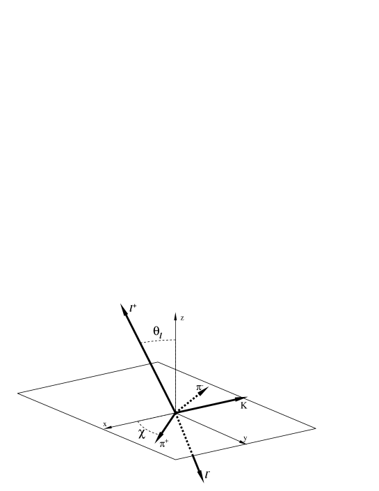
In order to extract information on the spin of the X𝑋X particle, we re-analyze the BXK𝐵𝑋𝐾B\to XK data published in Ref. Choi:2011fc (for XJ/ψπ+π𝑋𝐽𝜓superscript𝜋superscript𝜋X\to J/\psi\;\pi^{+}\pi^{-}) and in Ref. delAmoSanchez:2010jr (for XJ/ψπ+ππ0𝑋𝐽𝜓superscript𝜋superscript𝜋superscript𝜋0X\to J/\psi\;\pi^{+}\pi^{-}\pi^{0}). In particular, in the XJ/ψπ+π𝑋𝐽𝜓superscript𝜋superscript𝜋X\to J/\psi\;\pi^{+}\pi^{-} sample we consider the di-pion invariant mass (m2πsubscript𝑚2𝜋m_{2\pi}) and the angles defined in the X𝑋X rest frame in Ref. Rosner:2004ac and described in Fig 1: the angle between the J/ψ𝐽𝜓J/\psi and the direction opposite to K𝐾K (θXsubscript𝜃𝑋\theta_{X}), the angle between the π+superscript𝜋\pi^{+} and the direction opposite to K𝐾K (χ𝜒\chi), and the angle between the l+superscript𝑙l^{+} produced by the decay of the J/ψ𝐽𝜓J/\psi and the z𝑧z-axis of a coordinate system where the x𝑥x-axis is the direction opposite to the K𝐾K and the y𝑦y-axis is the component of π+superscript𝜋\pi^{+} orthogonal to K𝐾K (θlsubscript𝜃𝑙\theta_{l}). In the XJ/ψπ+ππ0𝑋𝐽𝜓superscript𝜋superscript𝜋superscript𝜋0X\to J/\psi\;\pi^{+}\pi^{-}\pi^{0}, instead, only the three pions invariant mass is considered (m3πsubscript𝑚3𝜋m_{3\pi}).

Refer to caption
Figure 1: Definition of the angles in XJ/ψπ+π𝑋𝐽𝜓superscript𝜋superscript𝜋X\to J/\psi\;\pi^{+}\pi^{-} Choi:2011fc .

With such distributions at hand the parameters of the model we have sensitivity upon are

  • the radii RJsubscript𝑅𝐽R_{J} (J=1,2𝐽12J=1,2) as defined in Eq. (7), to which only the invariant mass distributions are sensitive

  • the relative amplitudes and phases of the two contributions in case J=2𝐽2J=2 (g2ψVsubscript𝑔2𝜓𝑉g_{2\psi V} and g2ψVsubscriptsuperscript𝑔2𝜓𝑉g^{\prime}_{2\psi V} in Eq. (2)). We redefine

    g2ψξsubscript𝑔2𝜓𝜉\displaystyle g_{2\psi\xi} =r2ξcosθξ2,absentsubscript𝑟2𝜉subscript𝜃𝜉2\displaystyle=r_{2\xi}\cos\frac{\theta_{\xi}}{2}, g2ψξsubscriptsuperscript𝑔2𝜓𝜉\displaystyle g^{\prime}_{2\psi\xi} =r2ξsinθξ2eiφξabsentsubscript𝑟2𝜉subscript𝜃𝜉2superscript𝑒𝑖subscript𝜑𝜉\displaystyle=r_{2\xi}\sin\frac{\theta_{\xi}}{2}e^{i\varphi_{\xi}} (25)

    where ξ𝜉\xi can be ρ,ω𝜌𝜔\rho,\;\omega or ang, depending on whether we are fitting the m2πsubscript𝑚2𝜋m_{2\pi}, m3πsubscript𝑚3𝜋m_{3\pi}, or angular distributions respectively. The parameters θρsubscript𝜃𝜌\theta_{\rho} and φρsubscript𝜑𝜌\varphi_{\rho} satisfy θρ=θangsubscript𝜃𝜌subscript𝜃ang\theta_{\rho}=\theta_{\text{ang}} and φρ=φangsubscript𝜑𝜌subscript𝜑ang\varphi_{\rho}=\varphi_{\text{ang}} since in the ρ𝜌\rho channel we have information on both mass spectrum and angular distributions. Only the angular distributions are sensitive to the θ𝜃\theta and φ𝜑\varphi parameters

  • the overall normalizations, r2ξsubscript𝑟2𝜉r_{2\xi} and r1ξsubscript𝑟1𝜉r_{1\xi} (=g1ψρabsentsubscript𝑔1𝜓𝜌=g_{1\psi\rho} in Eq. ((1))). It has to be noted that the normalization depends on the distributions being studied

Given the different sensitivities of the mass and angle distributions and the computational complexity of the angular fits, the combined fits are performed in three steps: i)i) the invariant mass distributions are fitted letting all parameters float, ii)ii) the fits to the three angular distributions are performed fixing the RJsubscript𝑅𝐽R_{J} parameters to the results obtained in the previous fits, iii)iii) the invariant mass fits are repeated by fixing the θρsubscript𝜃𝜌\theta_{\rho} and φρsubscript𝜑𝜌\varphi_{\rho} distributions to the results of the angular fits. φωsubscript𝜑𝜔\varphi_{\omega} and θωsubscript𝜃𝜔\theta_{\omega} are always set to zero.

Mass and widths of the ρ𝜌\rho, ω𝜔\omega, and X𝑋X are fixed. To account for the X𝑋X width in the invariant mass distributions, we extract randomly the values of the mass of the X𝑋X from a Breit-Wigner centered at mX=3872MeVsubscript𝑚𝑋3872MeVm_{X}=3872\,\textrm{MeV} with ΓX=1.7MeVsubscriptΓ𝑋1.7MeV\Gamma_{X}=1.7\,\textrm{MeV} review , accepting only those values kinematically consistent with the decay of interest.

Finally, since as described in Appendix B the invariant mass fits return consistent results with either the n=1𝑛1n=1 or the n=2𝑛2n=2 hypotheses (where n𝑛n is defined in Eq. (7)) we will only report results with n=1𝑛1n=1.

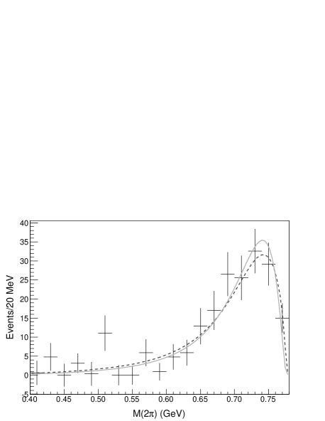
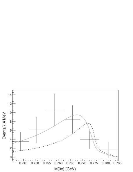
The resulting fits are shown in Figs. 2 and  3 and the fitted parameters are summarized in Tab. 1. It is interesting to note that the radii, which are the fit parameters with a physical content, have reasonably small errors and get values consistent with 111 fm, the size scale of a standard hadron. Here it is hard to judge if we are probing the size of the X𝑋X, in which case we would say that the results obtained for R𝑅R disfavor a large (10similar-toabsent10\sim 10 fm) loosely bound molecule loose , or the size of the interaction making the X𝑋X decay into J/ψ+V𝐽𝜓𝑉J/\psi+V. For sure the loosely bound molecule is requested to have a large wave function at the origin to make such a decay possible 444Moreover we remind that loosely bound molecules are very difficult to be produced with high cross sections at hadron colliders noigrin if not invoking final state interactions effect artoise .. On the other hand in any compact multiquark model the decay into J/ψ𝐽𝜓J/\psi does not require special conditions.

1++superscript1absent1^{++} (dashed curve) 2+superscript2absent2^{-+} (solid curve)
rJρsubscript𝑟𝐽𝜌r_{J\rho} 0.089±0.006plus-or-minus0.0890.0060.089\pm 0.006 a.u. 0.69±0.13plus-or-minus0.690.130.69\pm 0.13 a.u.
rJωsubscript𝑟𝐽𝜔r_{J\omega} 0.0026±0.0003plus-or-minus0.00260.00030.0026\pm 0.0003 a.u. 0.030±0.016plus-or-minus0.0300.0160.030\pm 0.016 a.u.
rJangsubscript𝑟𝐽angr_{J\text{ang}} 1.32±0.4plus-or-minus1.320.41.32\pm 0.4 a.u. 1.03±0.04plus-or-minus1.030.041.03\pm 0.04 a.u.
θρsubscript𝜃𝜌\theta_{\rho} - (254±16)superscriptplus-or-minus25416(254\pm 16)^{\circ}
φρsubscript𝜑𝜌\varphi_{\rho} - (14±60)superscriptplus-or-minus1460(14\pm 60)^{\circ}
RJsubscript𝑅𝐽R_{J} 1.6±0.3GeV1plus-or-minus1.60.3superscriptGeV11.6\pm 0.3\,\textrm{GeV}^{-1} 5.6±0.8GeV1plus-or-minus5.60.8superscriptGeV15.6\pm 0.8\,\textrm{GeV}^{-1}
χ2/DOFsuperscript𝜒2DOF\chi^{2}/\textrm{DOF} 31.8/3631.83631.8/36 37.3/3337.33337.3/33
P(χ2)𝑃superscript𝜒2P(\chi^{2}) 67%percent6767\% 28%percent2828\%
Table 1: Fit results for the two JPCsuperscript𝐽𝑃𝐶J^{PC} assignments.
Refer to caption
Refer to caption
Figure 2: Fit to the m2πsubscript𝑚2𝜋m_{2\pi} (left) and m3πsubscript𝑚3𝜋m_{3\pi} (right) distributions as described in the text, with the n=1𝑛1n=1 model. The dashed curve refers to the 1++superscript1absent1^{++} hypothesis whereas the solid one is for the 2+superscript2absent2^{-+}.
Refer to caption
Refer to caption
Refer to caption
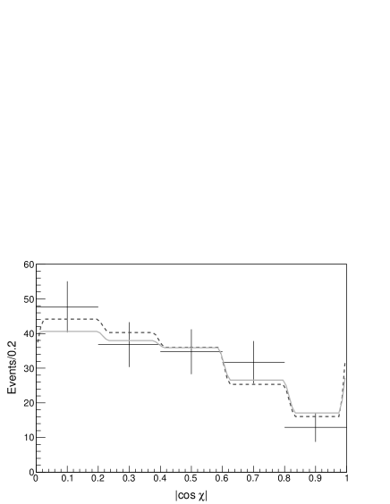
Figure 3: Fit to the angular distributions in XJ/ψπ+π𝑋𝐽𝜓superscript𝜋superscript𝜋X\to J/\psi\,\pi^{+}\pi^{-} decays as described in the text. The dashed curve refers to the 1++superscript1absent1^{++} hypothesis whereas the solid one is for the 2+superscript2absent2^{-+}.

IV.1 Statistical interpretation

The naïve approach to evaluate the likelihood of the two spin hypotheses would be to consider the χ2superscript𝜒2\chi^{2} of the fits, obtained by adding the contributions from all the distributions, and to compare them with the number of degrees of freedom. In our case this would return a χ2/DOF=31.8/36superscript𝜒2DOF31.836\chi^{2}/\textrm{DOF}=31.8/36 for the 1++superscript1absent1^{++} hypothesis and χ2/DOF=37.3/33superscript𝜒2DOF37.333\chi^{2}/\textrm{DOF}=37.3/33 for the 2+superscript2absent2^{-+} hypothesis. The probability of obtaining a worse value is P(χ2)=χ2PDF(x,NDOF)𝑑x=67%𝑃superscript𝜒2superscriptsubscriptsuperscript𝜒2PDF𝑥subscript𝑁DOFdifferential-d𝑥percent67P(\chi^{2})=\int_{\chi^{2}}^{\infty}{\rm PDF}(x,N_{\rm DOF})dx=67\% and 28%percent2828\% respectively, i.e., both hypotheses seem to fit data well.

Nonetheless this conclusion would not consider two effects. First, the overall good agreements is caused by the fact that we are simultaneously considering the distributions which favor the 1++superscript1absent1^{++} hypothesis (θX,χ,θlsubscript𝜃𝑋𝜒subscript𝜃𝑙\theta_{X},\chi,\theta_{l}) and the one which favors the 2+superscript2absent2^{-+} hypothesis (m3πsubscript𝑚3𝜋m_{3\pi}). This can be qualitatively seen in the fit results (Figs. 2 and 3) and in the P(χ2)𝑃superscript𝜒2P(\chi^{2}) values obtained on each fitted distribution as listed in Tab. 2. Then, a large number of degrees of freedom are not sensitive to the spin of the X𝑋X and therefore wash out the overall χ2superscript𝜒2\chi^{2}. This is the case for the m2πsubscript𝑚2𝜋m_{2\pi} distribution, which is sensitive only to the radii, but not to the spin.

To quantify this latter statement and develop a sounder statistical analysis, we performed a Monte Carlo (MC) study. We generate N𝑁N data samples with the same number of events as the experimental samples and take into account the background, the statistical fluctuations, and the uncertainties in the model parameters. The simulations can be performed either by making the hypothesis that the X𝑋X is truly a 1++superscript1absent1^{++} state or a 2+superscript2absent2^{-+} state.

As the starting point of the simulation for a given J𝐽J and n𝑛n hypothesis we take the corresponding model extracting sample by sample the parameters according to the result of the combined fit to the data. The invariant mass MC samples are generated by filling the bins bisubscript𝑏𝑖b_{i} according to Poisson distributions with mean values μisubscript𝜇𝑖\mu_{i} corresponding, bin per bin, to the sum of the values expected from the model and the experimental background. The angular pseudodata are generated as MC unweighted events.

After the extraction this background is treated in the same way as the data, subtracted in the case of the invariant mass distributions and accounted for in the fits in the case of the angular distributions.

The N𝑁N data samples obtained with this procedure are then analyzed with the same fitting function and statistical analysis as the experimental data.

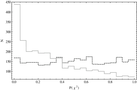
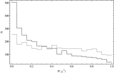
With such a tool, we first show the P(χ2)𝑃superscript𝜒2P(\chi^{2}) values obtained on the m2πsubscript𝑚2𝜋m_{2\pi} fits (Fig. 4) performed by generating the MC events with both the spin hypotheses and by fitting them either with the correct or the wrong hypothesis. These figures show that even when fitting with the incorrect X𝑋X spin the fit would return a good P(χ2)𝑃superscript𝜒2P(\chi^{2}). We therefore conclude that m2πsubscript𝑚2𝜋m_{2\pi} is not sensitive to the X𝑋X spin.

Refer to caption
Refer to caption
Figure 4: Distribution of the P(χ2)𝑃superscript𝜒2P(\chi^{2}) resulting from the fits to m2πsubscript𝑚2𝜋m_{2\pi} in MC samples generated assuming 1++superscript1absent1^{++} (left) and 2+superscript2absent2^{-+} (right). The solid (dashed) histogram corresponds to the fit to the 2+superscript2absent2^{-+} (1++superscript1absent1^{++}) model.

Since we need the invariant mass distributions to perform the combined fit to constraint the RJsubscript𝑅𝐽R_{J} variables, we developed a more robust method of testing the hypotheses by using as estimator the difference between the χ2superscript𝜒2\chi^{2} obtained from the combined fits performed under the two J𝐽J hypotheses Lyons:2008zz

Δχ2=χ2(1++)χ2(2+)Δsuperscript𝜒2superscript𝜒2superscript1absentsuperscript𝜒2superscript2absent\Delta\chi^{2}=\chi^{2}\left(1^{++}\right)-\chi^{2}\left(2^{-+}\right) (26)

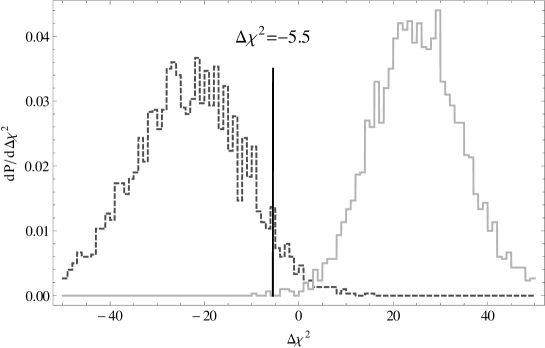
Fig. 5 shows that the distribution of such a variable is peaked around a negative value when the MC samples are generated with 1++superscript1absent1^{++} and, viceversa, it is peaked around a positive value when the samples are generated with 2+superscript2absent2^{-+}. These distributions are used to calculate the fraction of samples in which Δχ2Δsuperscript𝜒2\Delta\chi^{2} has a value larger (for 1++superscript1absent1^{++}) or smaller (for 2+superscript2absent2^{-+}) than the one obtained on data. This fraction, that we call CL, estimates the probability of the hypothesis.

Given that in the combined fit Δχ2=5.5Δsuperscript𝜒25.5\Delta\chi^{2}=-5.5, the 2+superscript2absent2^{-+} hypothesis is excluded at 99.9% C.L., while the 1++superscript1absent1^{++} hypothesis has a C.L. of 5.5%. The different conclusion with respect to the naïve expectations is due to the fact that individual χ2superscript𝜒2\chi^{2} values account only for the agreement of the data with the specific hypothesis under test. The Δχ2Δsuperscript𝜒2\Delta\chi^{2} approach instead also considers the level of agreement with the other hypothesis, weighting the degrees of freedom with their power to discriminate among the two hypotheses.
Refer to caption
Figure 5: Distribution of the Δχ2=χ2(1++)χ2(2+)Δsuperscript𝜒2superscript𝜒2superscript1absentsuperscript𝜒2superscript2absent\Delta\chi^{2}=\chi^{2}(1^{++})-\chi^{2}(2^{-+}) resulting from the combined fits to Monte Carlo data samples with n=1𝑛1n=1. The solid (dashed) histogram corresponds to events generated assuming the X𝑋X to be a 2+superscript2absent2^{-+} (1++superscript1absent1^{++}) state. We mark with a line the position of the experimental Δχ2Δsuperscript𝜒2\Delta\chi^{2}.

IV.2 Fits on sub-samples

The Δχ2Δsuperscript𝜒2\Delta\chi^{2} interpretation of the combined fit shows that even the agreement of the data with the 1++superscript1absent1^{++} hypothesis is marginal and the fit results seem to hint that the disagreement concentrates in the m3πsubscript𝑚3𝜋m_{3\pi} distribution (see Fig. 2). To quantify this statement we have performed the toy MC analysis on the Δχ2Δsuperscript𝜒2\Delta\chi^{2} value obtained separately on the m3πsubscript𝑚3𝜋m_{3\pi} distribution (obtained on the XJ/ψπ+ππ0𝑋𝐽𝜓superscript𝜋superscript𝜋superscript𝜋0X\to J/\psi\;\pi^{+}\pi^{-}\pi^{0} sample) and on the combination of the other distributions (obtained on the XJ/ψπ+π𝑋𝐽𝜓superscript𝜋superscript𝜋X\to J/\psi\;\pi^{+}\pi^{-} sample). The results, listed in Tab. 2, show that the fits to the XJ/ψπ+π𝑋𝐽𝜓superscript𝜋superscript𝜋X\to J/\psi\;\pi^{+}\pi^{-} distributions (second row) exclude the 2+superscript2absent2^{-+} hypothesis and have an agreement with the 1++superscript1absent1^{++} hypothesis at 23% C.L., while conversely the XJ/ψπ+ππ0𝑋𝐽𝜓superscript𝜋superscript𝜋superscript𝜋0X\to J/\psi\;\pi^{+}\pi^{-}\pi^{0} data (third row) favor the 2+superscript2absent2^{-+} at 81% and exclude the 1++superscript1absent1^{++} hypothesis at 99.9% C.L. The two samples return therefore inconsistent answers.

Finally, in order to compare directly with Ref. Hanhart:2011tn we report in Tab. 2 also the results performed using exclusively the two invariant mass distributions or the three angular distributions. Also here the former give a clear indication in favor of the 2+superscript2absent2^{-+} hypothesis, the latter in favor of the 1++superscript1absent1^{++} hypothesis. The different conclusion with respect to Ref. Hanhart:2011tn comes both from a different theoretical model and from the appropriate treatment of the degrees of freedom with no sensitivity to the spin of the X𝑋X.

1++superscript1absent1^{++} (dashed curve) 2+superscript2absent2^{-+} (solid curve)
combined χ2/DOF=31.8/36superscript𝜒2DOF31.836\chi^{2}/\text{DOF}=31.8/36 χ2/DOF=37.3/33superscript𝜒2DOF37.333\chi^{2}/\text{DOF}=37.3/33
P(χ2)=67%𝑃superscript𝜒2percent67P\left(\chi^{2}\right)=67\% P(χ2)=28%𝑃superscript𝜒2percent28P\left(\chi^{2}\right)=28\%
CL=5.5%𝐶𝐿percent5.5CL=5.5\% CL=0.1%𝐶𝐿percent0.1CL=0.1\%
2π2𝜋2\pi (angular + mass) χ2/DOF=20.9/31superscript𝜒2DOF20.931\chi^{2}/\text{DOF}=20.9/31 χ2/DOF=34.7/29superscript𝜒2DOF34.729\chi^{2}/\text{DOF}=34.7/29
P(χ2)=91%𝑃superscript𝜒2percent91P\left(\chi^{2}\right)=91\% P(χ2)=21%𝑃superscript𝜒2percent21P\left(\chi^{2}\right)=21\%
CL=23%𝐶𝐿percent23CL=23\% CL<0.1%𝐶𝐿percent0.1CL<0.1\%
3π3𝜋3\pi (mass) χ2/DOF=9.9/4superscript𝜒2DOF9.94\chi^{2}/\text{DOF}=9.9/4 χ2/DOF=1.5/3superscript𝜒2DOF1.53\chi^{2}/\text{DOF}=1.5/3
P(χ2)=4%𝑃superscript𝜒2percent4P\left(\chi^{2}\right)=4\% P(χ2)=68%𝑃superscript𝜒2percent68P\left(\chi^{2}\right)=68\%
CL=0.1%𝐶𝐿percent0.1CL=0.1\% CL=81%𝐶𝐿percent81CL=81\%
combined (only mass) χ2/DOF=25.2/22superscript𝜒2DOF25.222\chi^{2}/\text{DOF}=25.2/22 χ2/DOF=17.7/20superscript𝜒2DOF17.720\chi^{2}/\text{DOF}=17.7/20
P(χ2)=29%𝑃superscript𝜒2percent29P\left(\chi^{2}\right)=29\% P(χ2)=61%𝑃superscript𝜒2percent61P\left(\chi^{2}\right)=61\%
CL=0.1%𝐶𝐿percent0.1CL=0.1\% CL=46%𝐶𝐿percent46CL=46\%
2π2𝜋2\pi (only angular) χ2/DOF=6.6/14superscript𝜒2DOF6.614\chi^{2}/\text{DOF}=6.6/14 χ2/DOF=19.6/12superscript𝜒2DOF19.612\chi^{2}/\text{DOF}=19.6/12
P(χ2)=95%𝑃superscript𝜒2percent95P\left(\chi^{2}\right)=95\% P(χ2)=7.6%𝑃superscript𝜒2percent7.6P\left(\chi^{2}\right)=7.6\%
CL=27%𝐶𝐿percent27CL=27\% CL<0.1%𝐶𝐿percent0.1CL<0.1\%
Table 2: Results of the Toy MC

V Conclusions

We re-analyzed the XJ/ψπ+ππ0𝑋𝐽𝜓superscript𝜋superscript𝜋superscript𝜋0X\to J/\psi\;\pi^{+}\pi^{-}\pi^{0} and XJ/ψπ+π𝑋𝐽𝜓superscript𝜋superscript𝜋X\to J/\psi\;\pi^{+}\pi^{-} invariant mass and angle distributions published by the Belle Choi:2011fc and BaBar delAmoSanchez:2010jr collaborations respectively, with the goal to extract the most information about the spin of the X𝑋X particle.

With respect to the existing analyzes, we have improved two aspects. On one side, the X𝑋X decay amplitudes are parameterized by effective strong couplings, weighting terms written as products of momenta and polarizations as dictated by Lorentz invariance, and parity considerations in a model independent way. The strong couplings are given a momentum dependency according to the model defined in Eq. (7). This requires the introduction of an additional parameter R𝑅R which can be related to the finite size of hadrons in the interaction region. The results, shown in Tab. 1, are consistent with R𝑅R of the order of 1 fm. The treatment is fully relativistic and particularly appropriate for angular analyses.

On the other side, in order to properly account for the sensitivities to the X𝑋X spin of the considered distributions, we pursue a statistical approach based on Monte Carlo simulations.

We performed i)i) a global fit based on the whole information available from the 2π2𝜋2\pi, 3π3𝜋3\pi invariant mass spectra and the angular distributions of the XJ/ψρ𝑋𝐽𝜓𝜌X\to J/\psi\;\rho decays, ii)ii) two separated fits relative to the channels J/ψρ𝐽𝜓𝜌J/\psi\;\rho (where we do the combined fit of the angular and invariant mass distributions) and J/ψω𝐽𝜓𝜔J/\psi\;\omega (fitting only the invariant mass distribution). We also studied the fit to the invariant mass and the angular distributions separately.

The combined fit i)i) excludes the 2+superscript2absent2^{-+} hypothesis at 99.9%percent99.999.9\% C.L., but returns a probability of only 5.5%percent5.55.5\% of the 1++superscript1absent1^{++} hypothesis being correct. The separate fits ii)ii), return a clear a preference for the 1++superscript1absent1^{++} hypothesis in the J/ψρ𝐽𝜓𝜌J/\psi\;\rho channel with a probability of 23% and an 81% preference for the 2+superscript2absent2^{-+} assignment in the J/ψω𝐽𝜓𝜔J/\psi\;\omega channel, with very strong exclusions of other hypotheses. Such results go in the direction of two different assignments for the two samples, which can lead to a host of interesting considerations.

Acknowledgements

We would like to thank F.C. Porter for the discussion on the statistical approach, and F. Renga for the analysis of experimental data about the width of the X𝑋X. We also wish to thank C. Sabelli for her collaboration in the early stages of this work. The work of F. P. was supported by the Research Executive Agency (REA) of the European Union under the Grant Agreement number PITN-GA-2010-264564 (LHCPhenoNet).

Appendix A ρ𝜌\rho-ω𝜔\omega mixing

As discussed in Sec. III, the isosping-violating ρ𝜌\rho-ω𝜔\omega mixing introduces a correction near the pole of the ω𝜔\omega, without affecting the core of our analysis. Moreover, we found that the mixing improves the quality of the fit of 2+superscript2absent2^{-+} and worsens the 1++superscript1absent1^{++}.

First of all, we have to insert the mixing into (10) and (14). Following Ref. Hanhart:2011tn , we describe the decay ω2π𝜔2𝜋\omega\to 2\pi, as the oscillation ωρ2π𝜔𝜌2𝜋\omega\to\rho\to 2\pi, as explained in Fig. 6. We call ϵitalic-ϵ-\epsilon the coupling of the vertex ρω𝜌𝜔\rho\,\omega, whose value can be extracted by Hanhart:2011tn ; O'Connell:1995wf :

ϵmωmρΓρΓω(ω2π)3.4103GeV2italic-ϵsubscript𝑚𝜔subscript𝑚𝜌subscriptΓ𝜌subscriptΓ𝜔𝜔2𝜋3.4superscript103superscriptGeV2\epsilon\approx\sqrt{m_{\omega}\,m_{\rho}\,\Gamma_{\rho}\,\Gamma_{\omega}\,\mathcal{BR}(\omega\to 2\pi)}\approx 3.4\cdot 10^{-3}\,\textrm{GeV}^{2} (27)

.

The choice to treat the mixing reproduces naturally the phase of 95superscript9595^{\circ} of the complex mixing parameter used in Ref. Choi:2011fc .

Under the hypothesis 1++superscript1absent1^{++} we have

ψρ(q)|X=g1ψρTϵg1ψω1q2mω2+imωΓωTinner-product𝜓𝜌𝑞𝑋subscript𝑔1𝜓𝜌𝑇italic-ϵsubscript𝑔1𝜓𝜔1superscript𝑞2subscriptsuperscript𝑚2𝜔𝑖subscript𝑚𝜔subscriptΓ𝜔𝑇\langle\psi\,\rho(q)|X\rangle=g_{1\psi\rho}\,T-\epsilon\,g_{1\psi\omega}\frac{1}{q^{2}-m^{2}_{\omega}+im_{\omega}\Gamma_{\omega}}T (28)

where T𝑇T is the S-wave scalar described in (1). Similarly for 2+superscript2absent2^{-+}

ψρ(q)|X=(g2ψρTA+g2ψρTB)ϵg2ψωTA+g2ψωTBq2mω2+imωΓωinner-product𝜓𝜌𝑞𝑋subscript𝑔2𝜓𝜌subscript𝑇𝐴superscriptsubscript𝑔2𝜓𝜌subscript𝑇𝐵italic-ϵsubscript𝑔2𝜓𝜔subscript𝑇𝐴superscriptsubscript𝑔2𝜓𝜔subscript𝑇𝐵superscript𝑞2superscriptsubscript𝑚𝜔2𝑖subscript𝑚𝜔subscriptΓ𝜔\langle\psi\,\rho(q)|X\rangle=\left(g_{2\psi\rho}\;T_{A}+g_{2\psi\rho}^{\prime}\;T_{B}\right)-\epsilon\,\frac{g_{2\psi\omega}\;T_{A}+g_{2\psi\omega}^{\prime}\;T_{B}}{q^{2}-m_{\omega}^{2}+im_{\omega}\Gamma_{\omega}} (29)

We can repeat the same argument for ψω(q)|Xinner-product𝜓𝜔𝑞𝑋\langle\psi\,\omega(q)|X\rangle by swapping the role of ρ𝜌\rho and ω𝜔\omega. The rest of Eqs. (13) and (17) (namely the Breit-Wigner and the decay into pions) is unchanged, because in this picture it is only the ρ𝜌\rho (resp. the ω𝜔\omega) which can decay in 2π2𝜋2\pi (3π3𝜋3\pi), being the mixing exhausted in the ψV|Xinner-product𝜓𝑉𝑋\langle\psi V|X\rangle matrix element.

ψρ|X=inner-product𝜓𝜌𝑋absent\displaystyle{\langle\psi\,\rho|X\rangle=\;} \Vertex(35,25)2 \Line(0,25)(35,25) \Line(35,25)(60,50) \Line(35,25)(60,0) \Text(0,27)[bl]X𝑋\scriptstyle{X}\Text(54,50)[rt]J/ψ𝐽𝜓\scriptstyle{J/\psi}\Text(52,0)[rb]ρ𝜌\scriptstyle{\rho} +\displaystyle{\,+\,} \Vertex(35,25)2 \Vertex(48,12)2 \Line(0,25)(35,25) \Line(35,25)(60,50) \Line(35,25)(60,0) \Text(0,27)[bl]X𝑋\scriptstyle{X}\Text(54,50)[rt]J/ψ𝐽𝜓\scriptstyle{J/\psi}\Text(53,0)[rb]ρ𝜌\scriptstyle{\rho}\Text(40,18)[rt]ω𝜔\scriptstyle{\omega}

Figure 6: Feynman diagrams of XJ/ψρ𝑋𝐽𝜓𝜌X\to J/\psi\,\rho including the ρ𝜌\rho-ω𝜔\omega mixing. The second diagram includes the coupling ϵitalic-ϵ\epsilon and the propagator of the ω𝜔\omega.

Moreover, if we take the mixing into account, the parameters rJρsubscript𝑟𝐽𝜌r_{J\rho} and rJωsubscript𝑟𝐽𝜔r_{J\omega} of the fit appear together in both channels; therefore we must impose their correct relative normalization. This can be solved by imposing that Γ(XJ/ψ 3π)/Γ(XJ/ψ 2π)=0.8±0.3Γ𝑋𝐽𝜓3𝜋Γ𝑋𝐽𝜓2𝜋plus-or-minus0.80.3\Gamma\left(X\to J/\psi\,3\pi\right)/\Gamma\left(X\to J/\psi\,2\pi\right)=0.8\pm 0.3 delAmoSanchez:2010jr ; review .

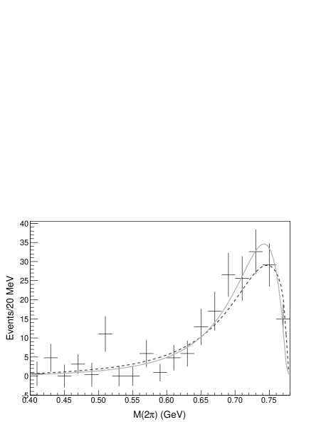
The angular distributions are unaffected by this term since they depend exclusively on the spin of the particles involved and not on the invariant mass spectrum. Therefore, to show the impact of the ρ𝜌\rho-ω𝜔\omega mixing we perform fits to the m2πsubscript𝑚2𝜋m_{2\pi} and m3πsubscript𝑚3𝜋m_{3\pi} distributions including this effect. The results are shown in Fig. 7, with the individual components detailed for the m2πsubscript𝑚2𝜋m_{2\pi} distribution in Fig. 8. The resulting values of the radii vary from R1=1.6±0.3subscript𝑅1plus-or-minus1.60.3R_{1}=1.6\pm 0.3 to R1=1.1±0.4subscript𝑅1plus-or-minus1.10.4R_{1}=1.1\pm 0.4 and from R2=5.6±0.8subscript𝑅2plus-or-minus5.60.8R_{2}=5.6\pm 0.8 to R2=4.5±0.7subscript𝑅2plus-or-minus4.50.7R_{2}=4.5\pm 0.7. As far as the hypothesis testing is concerned the χ2/DOFsuperscript𝜒2DOF\chi^{2}/\textrm{DOF} changes from 25.2/2225.22225.2/22 to 29.3/2229.32229.3/22 for the 1++superscript1absent1^{++} hypothesis, and from 17.7/2017.72017.7/20 to 16.0/2016.02016.0/20 for the 2+superscript2absent2^{-+} one. None of the relevant conclusions is altered by this small effect and we will therefore neglect it in the main analysis.
Refer to caption
Refer to caption
Figure 7: Fit including ρ𝜌\rho-ω𝜔\omega mixing to the m2πsubscript𝑚2𝜋m_{2\pi} (left) and m3πsubscript𝑚3𝜋m_{3\pi} (right) distributions, with the model with n=1𝑛1n=1. The dashed curve refers to the 1++superscript1absent1^{++} hypothesis, the solid one to the 2+superscript2absent2^{-+} one.

One could have thought that the presence of the narrow propagator of the ω𝜔\omega would have constrained the fit to raise a peak at mω=782subscript𝑚𝜔782m_{\omega}=782 MeV. The smallness of ϵitalic-ϵ\epsilon, instead, does not allow this, and the curve stays smooth at the pole, coherently with Refs. Abulencia:2005zc ; Choi:2011fc ; Hanhart:2011tn .

Refer to caption
Refer to caption
Figure 8: Fit to the m2πsubscript𝑚2𝜋m_{2\pi} distribution including ρ𝜌\rho-ω𝜔\omega mixing, with the model with n=1𝑛1n=1, and under the hypothesis JPC=1++superscript𝐽𝑃𝐶superscript1absentJ^{PC}=1^{++} (left) and 2+superscript2absent2^{-+} (right). The solid light curve is the ρ𝜌\rho contribution to the fit; the dotted light curve is the ω𝜔\omega contribution, and the dashed curve is the interference term. The darker curve is the sum of all contributions.

Appendix B n=2𝑛2n=2 case

The theoretical model chosen for the fits described in this paper does not specify the value of n𝑛n in Eq. (7), and it is therefore a free parameter of the model itself. Before adopting n=1𝑛1n=1 for the rest of our considerations, we have performed a check on the dependence of the results on the choice of n𝑛n.

Since the angular distributions have shown a scarce dependence on R𝑅R, we fitted the invariant mass spectra with n=2𝑛2n=2 comparing the result with the n=1𝑛1n=1 case. The results are shown in Fig. 9. The resulting values of the radii vary from R1=1.6±0.3subscript𝑅1plus-or-minus1.60.3R_{1}=1.6\pm 0.3 to R1=1.1±0.2subscript𝑅1plus-or-minus1.10.2R_{1}=1.1\pm 0.2 and from R2=5.6±0.8subscript𝑅2plus-or-minus5.60.8R_{2}=5.6\pm 0.8 to R2=2.8±0.3subscript𝑅2plus-or-minus2.80.3R_{2}=2.8\pm 0.3. As far as the hypothesis testing is concerned the χ2/DOFsuperscript𝜒2DOF\chi^{2}/\textrm{DOF} changes from 25.2/2225.22225.2/22 to 24.8/2224.82224.8/22 for the 1++superscript1absent1^{++} hypothesis, and from 17.7/2017.72017.7/20 to 18.9/2018.92018.9/20 for the 2+superscript2absent2^{-+} one. Also in this case none of the relevant conclusions is altered.

Refer to caption
Refer to caption
Figure 9: Fit to the m2πsubscript𝑚2𝜋m_{2\pi} (left) and m3πsubscript𝑚3𝜋m_{3\pi} (right) distributions as described in the text, with the model with n=2𝑛2n=2. The dashed curve refers to the 1++superscript1absent1^{++} hypothesis, the solid one is for the 2+superscript2absent2^{-+} one.

References

  • (1) P. del Amo Sanchez et al. [BABAR Collaboration], Phys. Rev. D 82 (2010) 011101 [arXiv:1005.5190 [hep-ex]].
  • (2) S. -K. Choi, S. L. Olsen, K. Trabelsi, I. Adachi, H. Aihara, K. Arinstein, D. M. Asner and T. Aushev et al., Phys. Rev. D 84 (2011) 052004 [arXiv:1107.0163 [hep-ex]].
  • (3) A. Abulencia et al. [CDF Collaboration], Phys. Rev. Lett.  98 (2007) 132002 [arXiv:hep-ex/0612053].
  • (4) F. Brazzi, B. Grinstein, F. Piccinini, A. D. Polosa and C. Sabelli, Phys. Rev. D 84 (2011) 014003 [arXiv:1103.3155 [hep-ph]].
  • (5) C. Hanhart, Y. .S. Kalashnikova, A. E. Kudryavtsev and A. V. Nefediev, Phys. Rev. D 85 (2012) 011501 [arXiv:1111.6241 [hep-ph]].
  • (6) A. Abulencia et al. [CDF Collaboration], Phys. Rev. Lett.  96 (2006) 102002 [arXiv:hep-ex/0512074]. [hep-ex/0512074].
  • (7) J. L. Rosner, Phys. Rev. D 70 (2004) 094023 [arXiv:hep-ph/0408334].
  • (8) N. Drenska, R. Faccini, F. Piccinini, A.D. Polosa, F. Renga and C. Sabelli, Riv. Nuovo Cim.  033, 633 (2010) [arXiv:1006.2741 [hep-ph]].
  • (9) E. Braaten and M. Kusunoki, Phys. Rev. D 69, 074005 (2004) [arXiv:hep-ph/0311147]. S. Pakvasa and M. Suzuki, Phys. Lett. B 579, 67 (2004) [arXiv:hep-ph/0309294]. M. B. Voloshin, Phys. Lett. B 579, 316 (2004) [arXiv:hep-ph/0309307]. M. B. Voloshin, Phys. Lett. B 604, 69 (2004) [arXiv:hep-ph/0408321].
  • (10) C. Bignamini, B. Grinstein, F. Piccinini, A. D. Polosa and C. Sabelli, Phys. Rev. Lett.  103, 162001 (2009) [arXiv:0906.0882 [hep-ph]].
  • (11) P. Artoisenet and E. Braaten, Phys. Rev. D 81 (2010) 114018 [arXiv:0911.2016 [hep-ph]].
  • (12) L. Demortier, “P values and nuisance parameters”, into L. Lyons, (ed.), H. B. Prosper, (ed.) and A. De Roeck, (ed.), “Statistical issues for LHC physics. Proceedings, Workshop, PHYSTAT-LHC, Geneva, Switzerland, June 27-29, 2007”, [http://phystat-lhc.web.cern.ch/phystat-lhc/proceedings.html]
  • (13) H. B. O’Connell, B. C. Pearce, A. W. Thomas and A. G. Williams, Prog. Part. Nucl. Phys.  39 (1997) 201 [arXiv:hep-ph/9501251].