Critical two-point functions for long-range statistical-mechanical models in high dimensions

Abstract

We consider long-range self-avoiding walk, percolation and the Ising model on $\mathbb{Z}^{d}$ that are defined by power-law decaying pair potentials of the form $D(x)\asymp|x|^{-d-\alpha}$ with $\alpha>0$. The upper-critical dimension $d_{\mathrm{c}}$ is $2(\alpha\wedge 2)$ for self-avoiding walk and the Ising model, and $3(\alpha\wedge 2)$ for percolation. Let $\alpha\neq 2$ and assume certain heat-kernel bounds on the $n$-step distribution of the underlying random walk. We prove that, for $d>d_{\mathrm{c}}$ (and the spread-out parameter sufficiently large), the critical two-point function $G_{p_{\mathrm{c}}}(x)$ for each model is asymptotically $C|x|^{\alpha\wedge 2-d}$, where the constant $C\in(0,\infty)$ is expressed in terms of the model-dependent lace-expansion coefficients and exhibits crossover between $\alpha<2$ and $\alpha>2$. We also provide a class of random walks that satisfy those heat-kernel bounds.

and T1Supported in part by NSC Grant 99-2115-M-030-004-MY3 and in part by NSC Grant 102-2115-M-030-001-MY2. T2Supported in part by JSPS Grant-in-Aid for Young Scientists (B) 21740059 and in part by JSPS Grant-in-Aid for Scientific Research (C) 24540106.

1 Introduction

The two-point function is one of the key observables to understand phase transitions and critical behavior. For example, the two-point function for the Ising model indicates how likely the spins located at those two sites point in the same direction. If it decays fast enough to be summable, then there is no macroscopic order. The summability of the two-point function is lost as soon as the model parameter (e.g., temperature) is above the critical point and, therefore, it is naturally hard to investigate critical behavior.

The lace expansion is a powerful tool to rigorously prove mean-field behavior above the model-dependent critical dimension. The mean-field behavior here is for the two-point function at the critical point to exhibit similar behavior to the underlying random walk. It has been successful to prove such behavior for various statistical-mechanical models, such as self-avoiding walk, percolation, lattice trees/animals and the Ising model. The best lace-expansion result obtained so far is to identify an asymptotic expression ($={}$the Newtonian potential times a model-dependent constant) of the critical two-point function for finite-range models, such as the nearest-neighbor model. However, this ultimate goal has not been achieved before this paper for long-range models, especially when the 1-step distribution for the underlying random walk decays in powers of distance; only the infrared bound on the Fourier transform of the two-point function was available. This was partly because of our poor understanding of the long-range models in the $x$-space, not in the Fourier space. For example, the random-walk Green’s function is known to be asymptotically Newtonian/Riesz depending on the power of the aforementioned power-law decaying 1-step distribution, but we were unable to find optimal error estimates in the literature. Also, the subcritical two-point function is known to decay exponentially for the finite-range models, but this is not the case for the power-law decaying long-range models; as is shown in this paper, the decay rate of the subcritical two-point function is the same as the 1-step distribution of the underlying random walk.

Therefore, the goal of this paper is to overcome those difficulties and derive an asymptotic expression of the critical two-point function for the power-law decaying long-range models above the critical dimension, using the lace expansion. We would also like to investigate crossover in the asymptotic expression when the power of the 1-step distribution of the underlying random walk changes.

1.1 Models and known results

Self-avoiding walk (SAW) is a model for linear polymers. We define the two-point function for SAW on $\mathbb{Z}^{d}$ as

$$G_{p}^{\mathrm{SAW}}(x)=\sum_{\omega\dvtx o\to x}p^{|\omega|}\prod_{j=1}^{|\omega|}D(\omega_{j}-\omega_{j-1})\prod_{s<t}(1-\delta_{\omega_{s},\omega_{t}}),$$ (1)

where $p\geq 0$ is the fugacity, $|\omega|$ is the length of a path $\omega=(\omega_{0},\omega_{1},\ldots,\omega_{|\omega|})$ and $D\dvtx\mathbb{Z}^{d}\to[0,1]$ is the $\mathbb{Z}^{d}$-symmetric nondegenerate [i.e., $D(o)\neq 1$] 1-step distribution for the underlying random walk (RW); the contribution from the 0-step walk is considered to be $\delta_{o,x}$ by convention. If the indicator function $\prod_{s<t}(1-\delta_{\omega_{s},\omega_{t}})$ is replaced by 1, then $G_{p}^{\mathrm{SAW}}(x)$ turns into the RW Green’s function $G_{p}^{\mathrm{RW}}(x)$, whose radius of convergence $p_{\mathrm{c}}^{\mathrm{RW}}$ is 1, as $\chi_{p}^{\mathrm{RW}}\equiv\sum_{x\in\mathbb{Z}^{d}}G_{p}^{\mathrm{RW}}(x)=(1-p)^{-1}$ for $p<1$ and $\chi_{p}^{\mathrm{RW}}=\infty$ for $p\geq 1$. Therefore, the radius of convergence $p_{\mathrm{c}}^{\mathrm{SAW}}$ for $G_{p}^{\mathrm{SAW}}(x)$ is not less than 1. It is known that $\chi_{p}^{\mathrm{SAW}}\equiv\sum_{x\in\mathbb{Z}^{d}}G_{p}^{\mathrm{SAW}}(x)<\infty$ if and only if $p<p_{\mathrm{c}}^{\mathrm{SAW}}$ and diverges as $p\uparrow p_{\mathrm{c}}^{\mathrm{SAW}}$. Here, and in the remainder of the paper, we often use “$\equiv$” for definition.

Percolation is a model for random media. Each bond $\{u,v\}$, which is a pair of vertices in $\mathbb{Z}^{d}$, is either occupied or vacant independently of the other bonds. The probability that $\{u,v\}$ is occupied is defined to be $pD(v-u)$, where $p\geq 0$ is the percolation parameter. Since $D$ is a probability distribution, the expected number of occupied bonds per vertex equals $p\sum_{x\neq o}D(x)=p(1-D(o))$. The percolation two-point function $G_{p}^{\mathrm{perc}}(x)$ is defined to be the probability that there is a self-avoiding path of occupied bonds from $o$ to $x$; again by convention, $G_{p}^{\mathrm{perc}}(o)=1$.

The Ising model is a model for magnets. For $\Lambda\subset\mathbb{Z}^{d}$ and $\varphi=\{\varphi_{v}\}_{v\in\Lambda}\in\{\pm 1\}^{\Lambda}$, we define the Hamiltonian (under the free-boundary condition) as

$$H_{\Lambda}(\varphi)=-\sum_{\{u,v\}\subset\Lambda}J_{u,v}\varphi_{u}\varphi_{v},$$ (2)

where $J_{u,v}=J_{o,v-u}\geq 0$ is the ferromagnetic pair potential and inherits the properties of the given $D$, as explained below. The finite-volume two-point function at the inverse temperature $\beta\geq 0$ is defined as

$$\langle\varphi_{o}\varphi_{x}\rangle_{\beta,\Lambda}=\sum_{\varphi\in\{\pm 1\}^{\Lambda}}\varphi_{o}\varphi_{x}e^{-\beta H_{\Lambda}(\varphi)}\biggm{/}\sum_{\varphi\in\{\pm 1\}^{\Lambda}}e^{-\beta H_{\Lambda}(\varphi)}.$$ (3)

It is known that $\langle\varphi_{o}\varphi_{x}\rangle_{\beta,\Lambda}$ is increasing in $\Lambda\uparrow\mathbb{Z}^{d}$. Let $p=\sum_{x\in\mathbb{Z}^{d}}\tanh(\beta J_{o,x})$. The Ising two-point function $G_{p}^{\mathrm{Ising}}(x)$ is defined to be the increasing-volume limit of $\langle\varphi_{o}\varphi_{x}\rangle_{\beta,\Lambda}$:

$$G_{p}^{\mathrm{Ising}}(x)=\lim_{\Lambda\uparrow\mathbb{Z}^{d}}\langle\varphi_{o}\varphi_{x}\rangle_{\beta,\Lambda}.$$ (4)

Let $D(x)=p^{-1}\tanh(\beta J_{o,x})$.

For percolation and the Ising model, there is a model-dependent critical point $p_{\mathrm{c}}\geq 1$ (from now on, we omit the superscript, unless it causes any confusion) such that

$$\chi_{p} \equiv \sum_{x\in\mathbb{Z}^{d}}G_{p}(x)\cases{<\infty,&\quad$[p<p_{\mathrm{c}}]$,\cr=\infty,&\quad$[p\geq p_{\mathrm{c}}]$,}$$

$$\theta_{p} \equiv \sqrt{\lim_{|x|\to\infty}G_{p}(x)}\cases{=0,&\quad$[p<p_{\mathrm{c}}]$,\cr>0,&\quad$[p>p_{\mathrm{c}}]$.}$$

The order parameter $\theta_{p}^{\mathrm{perc}}$ is the probability that the occupied cluster of the origin is unbounded, while $\theta_{p}^{\mathrm{Ising}}$ is the spontaneous magnetization, which is the infinite-volume limit of the finite-volume single-spin expectation $\langle\varphi_{o}\rangle_{\beta,\Lambda}^{+}$ under the plus-boundary condition. The continuity of $\theta_{p}$ at $p=p_{\mathrm{c}}$ in a general setting is still a remaining issue.

We are interested in asymptotic behavior of $G_{p_{\mathrm{c}}}(x)$ as $|x|\to\infty$. For the “uniformly spread-out” finite-range models, for example, $D(x)={\mathbh 1}_{\{|x|=1\}}/\break(2d)$ or $D(x)={\mathbh 1}_{\{\|x\|_{\infty}\leq L\}}/(2L+1)^{d}$ for some $L\in[1,\infty)$, it has been proved h08 , hhs03 , s07 that, if $d>4$ for SAW and the Ising model and $d>6$ for percolation, and if $d$ or $L$ is sufficiently large (depending on the models), then there is a model-dependent constant $A$ ($=1$ for RW) such that

$$G_{p_{\mathrm{c}}}(x)\mathop{\sim}_{|x|\to\infty}\frac{a_{d}/\sigma^{2}}{A|x|^{d-2}},$$ (6)

where “$\sim$” means that the asymptotic ratio of the left-hand side to the right-hand side is 1, and

$$a_{d}=\frac{d\Gamma((d-2)/2)}{2\pi^{d/2}},\qquad\sigma^{2}\equiv\sum_{x\in\mathbb{Z}^{d}}|x|^{2}D(x)=O\bigl{(}L^{2}\bigr{)}.$$ (7)

This is a sufficient condition for the following mean-field behavior a82 , af86 , an84 , ba91 , ms93 :

$$\chi_{p}\mathop{\asymp}_{p\uparrow p_{\mathrm{c}}}(p_{\mathrm{c}}-p)^{-1},\qquad\theta_{p}\mathop{\asymp}_{p\downarrow p_{\mathrm{c}}}\cases{\displaystyle\sqrt{p-p_{\mathrm{c}}},&\quad[Ising],\cr\displaystyle p-p_{\mathrm{c}},&\quad[percolation],}$$ (8)

where “$\asymp$” means that the asymptotic ratio of the left-hand side to the right-hand side is bounded away from zero and infinity.

The proof of the above result is based on the lace expansion (e.g., hs90 , ms93 , s07 , s06 ). The core concept of the lace expansion is to systematically isolate interaction among individuals (e.g., mutual avoidance between distinct vertices for SAW or between distinct occupied pivotal bonds for percolation) and derive macroscopic recursive structure that yields the random-walk like behavior (6). When $d>d_{\mathrm{c}}$ and $d\vee L\gg 1$ (i.e., $d$ or $L$ sufficiently large depending on the models), there is enough room for those individuals to be away from each other, and the lace expansion converges hs90 , ms93 , s07 , s06 . The resultant recursion equation for $G_{p}$ is the following:

$$G_{p}(x)=\cases{\displaystyle\delta_{o,x}+\sum_{v\in\mathbb{Z}^{d}}pD(v)G_{p}(x-v),\qquad\mbox{[RW],}\vspace*{6pt}\cr\displaystyle\delta_{o,x}+\sum_{v\in\mathbb{Z}^{d}}\bigl{(}pD(v)+\pi_{p}(v)\bigr{)}G_{p}(x-v),\cr\hskip 156.0pt\mbox{[SAW],}\vspace*{6pt}\cr\displaystyle\pi_{p}(x)+\mathop{\sum_{u,v\in\mathbb{Z}^{d}}}_{(u\neq v)}\pi_{p}(u)pD(v-u)G_{p}(x-v),\cr\hskip 156.0pt\mbox{[Ising and percolation],}}$$ (9)

where $\pi_{p}$ is the lace-expansion coefficient. To treat all models simultaneously, we introduce the notation $f*g$ to denote the convolution of functions $f$ and $g$ in $\mathbb{Z}^{d}$:

$$(f*g)(x)=\sum_{v\in\mathbb{Z}^{d}}f(v)g(x-v).$$ (10)

Then the above identities can be simplified as (the spatial variables are omitted)

$$G_{p}=\cases{\displaystyle\delta+pD*G_{p},&\quad[RW],\vspace*{2pt}\cr\displaystyle\delta+(pD+\pi_{p})*G_{p},&\quad[SAW],\vspace*{2pt}\cr\displaystyle\pi_{p}+\pi_{p}*p\bigl{(}D-D(o)\delta\bigr{)}*G_{p},&\quad[Ising and percolation].}$$ (11)

Repeated use of these identities yields

$$G_{p}=1_{p}+\mathchar 261\relax_{p}*pD*G_{p},$$ (12)

where

$$\mathchar 261\relax_{p}(x)=\cases{\delta_{o,x},\qquad\mbox{[RW]},\vspace*{3pt}\cr\displaystyle\sum_{n=0}^{\infty}\pi_{p}^{*n}(x)\equiv\sum_{n=0}^{\infty}(\underbrace{\pi_{p}*\cdots*\pi_{p}}_{n\mbox{-}\mathrm{fold}})(x),\cr\hskip 44.0pt\mbox{[SAW],}\hskip 5.0pt\cr\displaystyle\sum_{n=1}^{\infty}\bigl{(}-pD(o)\bigr{)}^{n-1}\pi_{p}^{*n}(x),\cr\hskip 44.0pt\mbox{[Ising and percolation]}}$$ (13)

with the convention $f^{*0}(x)\equiv\delta_{o,x}$ for general $f$. When $d>d_{\mathrm{c}}$ and $d\vee L\gg 1$, there is a $\rho>0$ such that $|\mathchar 261\relax_{p_{\mathrm{c}}}(x)|$ is summable and decays as $|x|^{-d-2-\rho}$ h08 , hhs03 , s07 . The multiplicative constant $A$ in (6) and $p_{\mathrm{c}}$ can be represented in terms of $\mathchar 261\relax_{p_{\mathrm{c}}}(x)$ as

$$\qquad p_{\mathrm{c}}=\biggl{(}\sum_{x\in\mathbb{Z}^{d}}\mathchar 261\relax_{p_{\mathrm{c}}}(x)\biggr{)}^{-1},\qquad A=p_{\mathrm{c}}\biggl{(}1+\frac{p_{\mathrm{c}}}{\sigma^{2}}\sum_{x\in\mathbb{Z}^{d}}|x|^{2}\mathchar 261\relax_{p_{\mathrm{c}}}(x)\biggr{)}.$$ (14)

In this paper, we investigate long-range SAW, percolation and the Ising model on $\mathbb{Z}^{d}$ defined by power-law decaying pair potentials of the form $D(x)\asymp|x|^{-d-\alpha}$ with $\alpha>0$. For example, as in csI , csII , we can consider the following uniformly spread-out long-range $D$ with parameter $L\in[1,\infty)$:

$$D(x)=\frac{|\!|\!|{x}/L|\!|\!|_{1}^{-d-\alpha}}{\sum_{y\in\mathbb{Z}^{d}}|\!|\!|{y}/L|\!|\!|_{1}^{-d-\alpha}},$$ (15)

where $|\!|\!|x|\!|\!|_{\ell}=|x|\vee\ell$. As a result,

$$D(x)=O\bigl{(}L^{\alpha}\bigr{)}|\!|\!|x|\!|\!|_{L}^{-d-\alpha},$$ (16)

which we require throughout the paper (cf., Assumption 1.1 below). The goal is to see how the asymptotic expression (6) of $G_{p_{\mathrm{c}}}(x)$ changes depending on the value of $\alpha$. We note that (6) and (14) are invalid for $\alpha\leq 2$ because then $\sigma^{2}=\infty$.

Let

$$d_{\mathrm{c}}=\cases{2(\alpha\wedge 2),&\quad[SAW and Ising],\vspace*{2pt}\cr 3(\alpha\wedge 2),&\quad[percolation].}$$ (17)

It has been proved hhs08 that, for $d>d_{\mathrm{c}}$ and $L\gg 1$, the Fourier transform $\hat{G}_{p}(k)\equiv\sum_{x\in\mathbb{Z}^{d}}e^{ik\cdot x}G_{p}(x)$ for the long-range models is bounded above and below by a multiple of $\hat{G}_{\hat{p}}^{\mathrm{RW}}(k)\equiv(1-\hat{p}\hat{D}(k))^{-1}$ with $\hat{p}=p/p_{\mathrm{c}}$, uniformly in $p<p_{\mathrm{c}}$. Although this gives an impression of the similarity between $G_{p_{\mathrm{c}}}(x)$ and $G_{1}^{\mathrm{RW}}(x)$, it is still too weak to identify the asymptotic expression of $G_{p_{\mathrm{c}}}(x)$. The proof of the above Fourier-space result makes use of the following properties of $D$ that we make use of here as well: there are $v_{\alpha}=O(L^{\alpha\wedge 2})$ and $\varepsilon>0$ such that

$$\hat{D}(k) \equiv \sum_{x\in\mathbb{Z}^{d}}e^{ik\cdot x}D(x)$$

$$= 1-v_{\alpha}|k|^{\alpha\wedge 2}\times\cases{\displaystyle 1+O\bigl{(}(L|k|)^{\varepsilon}\bigr{)},&\quad$[\alpha\neq 2]$,\vspace*{4pt}\cr\displaystyle\log\frac{1}{L|k|}+O(1),&\quad$[\alpha=2]$.}$$

If $\alpha>2$, then $v_{\alpha}=\sigma^{2}/(2d)$. Moreover, if $L\gg 1$, then there is a constant $\Delta\in(0,1)$ such that

$$\bigl{\|}D^{*n}\bigr{\|}_{\infty}\leq O\bigl{(}L^{-d}\bigr{)}n^{-d/(\alpha\wedge 2)}\qquad[n\geq 1],$$

(20)

$$1-\hat{D}(k)\cases{<2-\Delta,&\quad$\bigl{[}k\in[-\pi,\pi]^{d}\bigr{]}$,\vspace*{4pt}\cr>\Delta,&\quad$\bigl{[}\|k\|_{\infty}\geq L^{-1}\bigr{]}$.}$$

All those properties hold for $D$ in (15) (cf., csI , csII , csIII ).

1.2 Main result

In addition to the above properties, the $n$-step transition probability obeys the following bound:

$$D^{*n}(x)\leq\frac{O(L^{\alpha\wedge 2})}{|\!|\!|x|\!|\!|_{L}^{d+\alpha\wedge 2}}n\times\cases{1,&\quad$[\alpha\neq 2]$,\vspace*{2pt}\cr\log|\!|\!|x|\!|\!|_{L},&\quad$[\alpha=2]$.}$$ (21)

This is due to the following two facts: (i) the contribution from the walks that have at least one step which is longer than $c|\!|\!|x|\!|\!|_{L}$ for a given $c>0$ is bounded by $O(L^{\alpha})n/|\!|\!|x|\!|\!|_{L}^{d+\alpha}$; (ii) the contribution from the walks whose $n$ steps are all shorter than $c|\!|\!|x|\!|\!|_{L}$ is bounded, due to the local CLT, by $O(\tilde{v}n)^{-d/2}e^{-|x|^{2}/O(\tilde{v}n)}\leq O(\tilde{v}n)/|\!|\!|x|\!|\!|_{L}^{d+2}$ (times an exponentially small normalization constant), where $\tilde{v}$ is the variance of the truncated 1-step distribution $\tilde{D}(y)\equiv D(y){\mathbh 1}_{\{|y|\leq c|x|\}}$ and equals

$$\tilde{v}=\sum_{y\in\mathbb{Z}^{d}}|y|^{2}\tilde{D}(y)\leq O\bigl{(}L^{\alpha\wedge 2}\bigr{)}\times\cases{|\!|\!|x|\!|\!|_{L}^{2-\alpha},&\quad$[\alpha<2]$,\vspace*{2pt}\cr\log|\!|\!|x|\!|\!|_{L},&\quad$[\alpha=2]$,\vspace*{2pt}\cr 1,&\quad$[\alpha>2]$.}$$ (22)

For $\alpha\neq 2$, inequality (21) is a discrete space–time version of the heat-kernel bound on the transition density $p_{s}(x)$ of an $\alpha$-stable/Gaussian process:

$$p_{s}(x)\equiv\int_{\mathbb{R}^{d}}\frac{\mathrm{d}^{d}k}{(2\pi)^{d}}e^{-ik\cdot x-s|k|^{\alpha\wedge 2}}\leq\frac{O(s)}{|x|^{d+\alpha\wedge 2}}.$$ (23)

In Section 2.1, we will show that the properties (16), (1.1) and (21) are sufficient to obtain an asymptotic expression of $G_{1}^{\mathrm{RW}}(x)$. However, these properties are not good enough to fully control error terms arising from convolutions of $D^{*n}(x)$ and $\mathchar 261\relax_{p}(x)$ in (13). To overcome this difficulty, we assume the following bound on the discrete derivative of the $n$-step transition probability:

$$\biggl{|}D^{*n}(x)-\frac{D^{*n}(x+y)+D^{*n}(x-y)}{2}\biggr{|}\leq\frac{O(L^{\alpha\wedge 2})|\!|\!|y|\!|\!|_{L}^{2}}{|\!|\!|x|\!|\!|_{L}^{d+\alpha\wedge 2+2}}n$$

(24)

$$\eqntext{\biggl{[}|y|\leq\dfrac 13|x|\biggr{]}.}$$ (25)

Here is the summary of the properties of $D$ that we use throughout the paper.

Assumption 1.1.

The $\mathbb{Z}^{d}$-symmetric 1-step distribution $D$ satisfies the properties (16), (1.1), (1.1), (21) and (1.2).

In Appendix, we will show that the following $D$ satisfies all properties in the above assumption:

$$D(x)=\sum_{t\in\mathbb{N}}U_{L}^{*t}(x)T_{\alpha}(t),$$ (26)

where $U_{L}$ is in a class of $\mathbb{Z}^{d}$-symmetric distributions on $\mathbb{Z}^{d}\cap[-L,L]^{d}$, and $T_{\alpha}$ is the stable distribution on $\mathbb{N}$ with parameter $\alpha/2\neq 1$.

Under the above assumption on $D$, we can prove the following theorem.

Theorem 1.2

Let $\alpha>0$, $\alpha\neq 2$ and

$$\gamma_{\alpha}=\frac{\Gamma((d-\alpha\wedge 2)/2)}{2^{\alpha\wedge 2}\pi^{d/2}\Gamma((\alpha\wedge 2)/2)}$$ (27)

and assume all properties of $D$ in Assumption 1.1. Then, for RW with $d>\alpha\wedge 2$ and any $L\geq 1$, and for SAW, percolation and the Ising model with $d>d_{\mathrm{c}}$ and $L\gg 1$, there are $\mu\in(0,\alpha\wedge 2)$ and $A=A(\alpha,d,L)\in(0,\infty)$ ($A\equiv 1$ for random walk) such that, as $|x|\to\infty$,

$$G_{p_{\mathrm{c}}}(x)=\frac{\gamma_{\alpha}/v_{\alpha}}{A|x|^{d-\alpha\wedge 2}}+\frac{O(L^{-\alpha\wedge 2+\mu})}{|x|^{d-\alpha\wedge 2+\mu}}.$$ (28)

As a result, by hhs08 , $\chi_{p}$ and $\theta_{p}$ exhibit the mean-field behavior (8). Moreover, $p_{\mathrm{c}}$ and $A$ can be expressed in term of $\mathchar 261\relax_{p}$ in (13) as

$$\qquad p_{\mathrm{c}}=\hat{\mathchar 261\relax}_{p_{\mathrm{c}}}(0)^{-1},\qquad A=p_{\mathrm{c}}+\cases{0,&\quad$[\alpha<2]$,\vspace*{5pt}\cr\displaystyle\frac{p_{\mathrm{c}}^{2}}{\sigma^{2}}\sum_{x}|x|^{2}\mathchar 261\relax_{p_{\mathrm{c}}}(x),&\quad$[\alpha>2]$.}$$ (29)

Remark 1.3.

(a) The finite-range models are formally considered as the $\alpha=\infty$ model. Indeed, the leading term in (28) for $\alpha>2$ is identical to (6).

(b) Following the argument in h08 , s07 , we can “almost” prove Theorem 1.2 for $\alpha>2$ without assuming the bounds on $D^{*n}(x)$. The shortcoming is the restriction $d>10$, not $d>6$, for percolation. This is due to the peculiar diagrammatic estimate in h08 , which we do not use in this paper.

(c) The asymptotic behavior of $G_{p_{\mathrm{c}}}(x)$ in (6) or (28) is a key element for the so-called 1-arm exponent to take on its mean-field value hhs?? , hhh11 , kn11 , s04 . For finite-range critical percolation, for example, the probability that $o\in\mathbb{Z}^{d}$ is connected to the surface of the $d$-dimensional ball of radius $r$ centered at $o$ is bounded above and below by a multiple of $r^{-2}$ in high dimensions kn11 . The value of the exponent may change in a peculiar way depending on the value of $\alpha$ hhh11 .

(d) As described in (29), the constant $A$ exhibits crossover between $\alpha<2$ and $\alpha>2$; in particular, $A=p_{\mathrm{c}}$ for $\alpha<2$ [cf., (LABEL:eq-bnabla-def) below]. According to some rough computations, it seems that the asymptotic expression of $G_{p_{\mathrm{c}}}(x)$ for $\alpha=2$ is a mixture of those for $\alpha<2$ and $\alpha>2$, with a logarithmic correction:

$$G_{p_{\mathrm{c}}}(x)\mathop{\sim}_{|x|\to\infty}\frac{\gamma_{2}/v_{2}}{p_{\mathrm{c}}|x|^{d-2}\log|x|}.$$ (30)

One of the obstacles to prove this conjecture is a lack of good control on convolutions of the RW Green’s function and the lace-expansion coefficients for $\alpha=2$. As hinted in the above expression, we may have to deal with logarithmic factors more actively than ever. We are currently working in this direction.

1.3 Notation and the organization

From now on, we distinguish $G_{p}^{\mathrm{RW}}$ from $G_{p}$ for the other three models, and define

$$S_{p}=G_{p}^{\mathrm{RW}}.$$ (31)

Here, and in the remainder of the paper, the spatial variables are sometimes omitted. For example,

$$S_{p}=\delta+pD*S_{p}$$ (32)

is the abbreviated version of the convolution equation

$$S_{p}(x)=\delta_{o,x}+(pD*S_{p})(x)=\delta_{o,x}+\sum_{y\in\mathbb{Z}^{d}}pD(y)S_{p}(x-y).$$ (33)

We also recall the notation

$$|\!|\!|x|\!|\!|_{\ell}=|x|\vee\ell.$$ (34)

The remainder of the paper is organized as follows. In Section 2, we prove the asymptotic expression (28) for $S_{1}$, as well as bounds on $S_{p}$ for $p\leq 1$ and some basic properties of $G_{p}$ for $p\leq p_{\mathrm{c}}$. Then, by using these facts and the diagrammatic bounds on the lace-expansion coefficients in hhs03 , s07 , we prove (28) for $G_{p_{\mathrm{c}}}$ in Section 3.

2 Preliminaries

In this section, we derive the asymptotic expression (28) for $S_{1}$, which will be restated as Proposition 2.1, and prove some properties of $G_{p}$ that will be used to prove Theorem 1.2 in Section 3.

2.1 Asymptotics of $S_{p}$

Proposition 2.1.

Let $\alpha>0$, $\alpha\neq 2$ and $d>\alpha\wedge 2$, and assume all properties but (1.2) in Assumption 1.1. Then there is a $\mu\in(0,\alpha\wedge 2)$ such that, for any $L\geq 1$, $p\leq 1$ and $\kappa>0$,

$$\delta_{o,x} \leq S_{p}(x)\leq\delta_{o,x}+\frac{O(L^{-\alpha\wedge 2})}{|\!|\!|x|\!|\!|_{L}^{d-\alpha\wedge 2}}\qquad\bigl{[}\forall x\in\mathbb{Z}^{d}\bigr{]},$$ (35)

$$S_{1}(x) = \frac{\gamma_{\alpha}/v_{\alpha}}{|x|^{d-\alpha\wedge 2}}+\frac{O(L^{-\alpha\wedge 2+\mu})}{|x|^{d-\alpha\wedge 2+\mu}}\qquad\bigl{[}|x|>L^{1+\kappa}\bigr{]},$$ (36)

where a constant in the $O(L^{-\alpha\wedge 2+\mu})$ term depends on $\kappa$.

Inequality (35) is an immediate result of (32), $p\leq 1$ and (1.1)–(21) as

$$0 \leq S_{p}(x)-\delta_{o,x}$$

$$\leq \sum_{n=1}^{\infty}D^{*n}(x)$$

$$\leq \frac{O(L^{\alpha\wedge 2})}{|\!|\!|x|\!|\!|_{L}^{d+\alpha\wedge 2}}\sum_{n=1}^{(|\!|\!|x|\!|\!|_{L}/L)^{\alpha\wedge 2}}n+O\bigl{(}L^{-d}\bigr{)}\sum_{n=(|\!|\!|x|\!|\!|_{L}/L)^{\alpha\wedge 2}}^{\infty}n^{-d/(\alpha\wedge 2)}$$

$$= \frac{O(L^{-\alpha\wedge 2})}{|\!|\!|x|\!|\!|_{L}^{d-\alpha\wedge 2}}.$$

To prove the asymptotic expression (36), we first rewrite $S_{1}(x)$ for $d>\alpha\wedge 2$ as

$$S_{1}(x) = \int_{[-\pi,\pi]^{d}}\frac{\mathrm{d}^{d}k}{(2\pi)^{d}}\frac{e^{-ik\cdot x}}{1-\hat{D}(k)}$$

$$= \int_{0}^{\infty}\mathrm{d}t\int_{[-\pi,\pi]^{d}}\frac{\mathrm{d}^{d}k}{(2\pi)^{d}}e^{-ik\cdot x-t(1-\hat{D}(k))}$$

$$= \int_{T}^{\infty}\mathrm{d}t\int_{[-\pi,\pi]^{d}}\frac{\mathrm{d}^{d}k}{(2\pi)^{d}}e^{-ik\cdot x-t(1-\hat{D}(k))}+I_{1}$$

for any $T\in(0,\infty)$, where

$$I_{1} = \int_{0}^{T}\mathrm{d}t\int_{[-\pi,\pi]^{d}}\frac{\mathrm{d}^{d}k}{(2\pi)^{d}}e^{-ik\cdot x-t(1-\hat{D}(k))}$$

$$= \int_{0}^{T}\mathrm{d}t\,e^{-t}\sum_{n=0}^{\infty}\frac{t^{n}}{n!}D^{*n}(x).$$

Next, we rewrite the large-$t$ integral as

$$\qquad\int_{T}^{\infty}\mathrm{d}t\int_{[-\pi,\pi]^{d}}\frac{\mathrm{d}^{d}k}{(2\pi)^{d}}e^{-ik\cdot x-t(1-\hat{D}(k))}=\int_{0}^{\infty}\mathrm{d}t\,p_{v_{\alpha}t}(x)+\sum_{j=2}^{5}I_{j},$$ (40)

where $p_{s}(x)$ is the transition density of an $\alpha$-stable/Gaussian process [cf., (23)], and for any $R\in(0,\pi)$,

$$I_{2} = -\int_{0}^{T}\mathrm{d}t\,p_{v_{\alpha}t}(x)\equiv-\int_{0}^{T}\mathrm{d}t\int_{\mathbb{R}^{d}}\frac{\mathrm{d}^{d}k}{(2\pi)^{d}}e^{-ik\cdot x-v_{\alpha}t|k|^{\alpha\wedge 2}},$$ (41)

$$I_{3} = \int_{T}^{\infty}\mathrm{d}t\int_{|k|\leq R}\frac{\mathrm{d}^{d}k}{(2\pi)^{d}}e^{-ik\cdot x}\bigl{(}e^{-t(1-\hat{D}(k))}-e^{-v_{\alpha}t|k|^{\alpha\wedge 2}}\bigr{)},$$ (42)

$$I_{4} = \int_{T}^{\infty}\mathrm{d}t\int_{[-\pi,\pi]^{d}}\frac{\mathrm{d}^{d}k}{(2\pi)^{d}}e^{-ik\cdot x-t(1-\hat{D}(k))}{\mathbh 1}_{\{|k|>R\}},$$ (43)

$$I_{5} = -\int_{T}^{\infty}\mathrm{d}t\int_{|k|>R}\frac{\mathrm{d}^{d}k}{(2\pi)^{d}}e^{-ik\cdot x-v_{\alpha}t|k|^{\alpha\wedge 2}}.$$ (44)

By using the identity

$$\int_{0}^{\infty}\mathrm{d}t\,e^{-v_{\alpha}t|k|^{\alpha\wedge 2}}$$

(45)

$$\qquad=\frac{1}{v_{\alpha}|k|^{\alpha\wedge 2}}=\frac{1}{v_{\alpha}\Gamma((\alpha\wedge 2)/2)}\int_{0}^{\infty}\mathrm{d}t\,t^{((\alpha\wedge 2)/2)-1}e^{-|k|^{2}t},$$

we obtain

$$\int_{0}^{\infty}\mathrm{d}t\,p_{v_{\alpha}t}(x)$$

$$\qquad=\frac{1}{v_{\alpha}\Gamma((\alpha\wedge 2)/2)}\int_{0}^{\infty}\mathrm{d}t\,t^{((\alpha\wedge 2)/2)-1}\int_{\mathbb{R}^{d}}\frac{\mathrm{d}^{d}k}{(2\pi)^{d}}e^{-|k|^{2}t-ik\cdot x}$$ (46)

$$\qquad=\frac{\gamma_{\alpha}/v_{\alpha}}{|x|^{d-\alpha\wedge 2}}.$$

As a result, we arrive at

$$S_{1}(x)=\frac{\gamma_{\alpha}/v_{\alpha}}{|x|^{d-\alpha\wedge 2}}+\sum_{j=1}^{5}I_{j}.$$ (47)

It remains to estimate $\sum_{j=1}^{5}I_{j}$. First, by (21) and (23), we can estimate $I_{1}+I_{2}$ for $|x|>L$ as

$$|I_{1}+I_{2}|\leq\frac{O(L^{\alpha\wedge 2})}{|x|^{d+\alpha\wedge 2}}\int_{0}^{T}\mathrm{d}t\,t\leq\frac{O(L^{\alpha\wedge 2})T^{2}}{|x|^{d+\alpha\wedge 2}}.$$ (48)

Let

$$\mu=\frac{2(\alpha\wedge 2)\varepsilon}{d+\alpha\wedge 2+\varepsilon},\qquad T=\biggl{(}\frac{|x|}{L}\biggr{)}^{\alpha\wedge 2-\mu/2}.$$ (49)

Then we obtain

$$|I_{1}+I_{2}|\leq\frac{O(L^{-\alpha\wedge 2+\mu})}{|x|^{d-\alpha\wedge 2+\mu}}.$$ (50)

Next, we estimate $I_{3}$. For small $R$, whose value will be determined shortly, we use (1.1) to obtain

$$\bigl{|}e^{-t(1-\hat{D}(k))}-e^{-v_{\alpha}t\bigr{|}k|^{\alpha\wedge 2}}|\leq O\bigl{(}L^{\alpha\wedge 2+\varepsilon}\bigr{)}t|k|^{\alpha\wedge 2+\varepsilon}e^{-v_{\alpha}t|k|^{\alpha\wedge 2}}.$$ (51)

Therefore, by (49),

$$|I_{3}| \leq O\bigl{(}L^{\alpha\wedge 2+\varepsilon}\bigr{)}\int_{T}^{\infty}\mathrm{d}t\,t\int_{|k|\leq R}\,\mathrm{d}^{d}k|k|^{\alpha\wedge 2+\varepsilon}e^{-v_{\alpha}t|k|^{\alpha\wedge 2}}$$

$$= O\bigl{(}L^{\alpha\wedge 2+\varepsilon}\bigr{)}\int_{T}^{\infty}\mathrm{d}t\,t\int_{0}^{v_{\alpha}tR^{\alpha\wedge 2}}\frac{\mathrm{d}r}{r}\biggl{(}\frac{r}{v_{\alpha}t}\biggr{)}^{(d+\alpha\wedge 2+\varepsilon)/(\alpha\wedge 2)}e^{-r}$$

$$\leq O\bigl{(}L^{\alpha\wedge 2+\varepsilon}\bigr{)}\int_{T}^{\infty}\mathrm{d}t\,t(v_{\alpha}t)^{-(d+\alpha\wedge 2+\varepsilon)/(\alpha\wedge 2)}$$

$$\leq O\bigl{(}L^{-d}\bigr{)}T^{1-((d+\varepsilon)/(\alpha\wedge 2))}=\frac{O(L^{-\alpha\wedge 2+\mu})}{|x|^{d-\alpha\wedge 2+\mu}}.$$

Finally we estimate $I_{4}+I_{5}$ and determine the value of $R$ during the course. First, by (1.1)–(1.1), we have

$$\qquad|I_{4}| \leq \int_{T}^{\infty}\mathrm{d}t\int_{[-\pi,\pi]^{d}}\frac{\mathrm{d}^{d}k}{(2\pi)^{d}}e^{-t(1-\hat{D}(k))}{\mathbh 1}_{\{|k|>R\}}$$

$$\hskip 66.5pt{}\times({\mathbh 1}_{\{\|k\|_{\infty}<L^{-1}\}}+{\mathbh 1}_{\{\|k\|_{\infty}\geq L^{-1}\}})$$

$$\leq \int_{T}^{\infty}\mathrm{d}t\biggl{(}\int_{|k|>R}\frac{\mathrm{d}^{d}k}{(2\pi)^{d}}e^{-tc(L|k|)^{\alpha\wedge 2}}+O(1)e^{-t\Delta}\biggr{)}$$

$$\leq O\bigl{(}L^{-d}\bigr{)}\int_{T}^{\infty}\mathrm{d}t\,t^{-d/(\alpha\wedge 2)}\Gamma\biggl{(}\frac{d}{\alpha\wedge 2};tc(LR)^{\alpha\wedge 2}\biggr{)}+O(1)e^{-T\Delta},$$

where $\Gamma(a;x)\equiv\int_{x}^{\infty}\mathrm{d}t\,t^{a-1}e^{-t}$ is the incomplete gamma function, which is bounded by $O(x^{a-1})e^{-x}$ for large $x$. Here, we choose $R$ to satisfy

$$tc(LR)^{\alpha\wedge 2}=\frac{2\varepsilon}{\alpha\wedge 2}\log t.$$ (54)

Then, for large $t$,

$$\Gamma\biggl{(}\frac{d}{\alpha\wedge 2};tc(LR)^{\alpha\wedge 2}\biggr{)}$$

$$\qquad\leq O\bigl{(}\bigl{(}tc(LR)^{\alpha\wedge 2}\bigr{)}^{(d/(\alpha\wedge 2))-1}\bigr{)}e^{-tc(LR)^{\alpha\wedge 2}}$$ (55)

$$\qquad=O\bigl{(}(\log t)^{(d/(\alpha\wedge 2))-1}\bigr{)}t^{-(2\varepsilon)/(\alpha\wedge 2)}\leq O\bigl{(}t^{-\varepsilon/(\alpha\wedge 2)}\bigr{)}.$$

Therefore, again by (49) [cf., (2.1)],

$$O\bigl{(}L^{-d}\bigr{)}\int_{T}^{\infty}\mathrm{d}t\,t^{-d/(\alpha\wedge 2)}\Gamma\biggl{(}\frac{d}{\alpha\wedge 2};tc(LR)^{\alpha\wedge 2}\biggr{)}$$

(56)

$$\qquad\leq O\bigl{(}L^{-d}\bigr{)}T^{1-((d+\varepsilon)/(\alpha\wedge 2))}=\frac{O(L^{-\alpha\wedge 2+\mu})}{|x|^{d-\alpha\wedge 2+\mu}}.$$

We can estimate $I_{5}$ in exactly the same way. The exponentially decaying term in (2.1) obeys the same bound, since, for sufficiently large $N$ (depending on $\kappa$),

$$e^{-T\Delta} \leq \frac{{}^{\exists}c_{N}}{T^{N}}=c_{N}L^{-d}T^{1-((d+\varepsilon)/(\alpha\wedge 2))}L^{d}T^{-(N+1-((d+\varepsilon)/(\alpha\wedge 2)))}$$

$$\leq c_{N}L^{-d}T^{1-((d+\varepsilon)/(\alpha\wedge 2))}L^{d-(N+1-((d+\varepsilon)/(\alpha\wedge 2)))(\alpha\wedge 2-\mu/2)\kappa}$$

$$\bigl{[}\because|x|>L^{1+\kappa}\Rightarrow T>L^{(\alpha\wedge 2-\mu/2)\kappa}\bigr{]}$$

$$\leq c_{N}L^{-d}T^{1-((d+\varepsilon)/(\alpha\wedge 2))}=\frac{O(L^{-\alpha\wedge 2+\mu})}{|x|^{d-\alpha\wedge 2+\mu}}.$$

Summarizing the above, we obtain that, for $|x|>L^{1+\kappa}$,

$$\Biggl{|}\sum_{j=1}^{5}I_{j}\Biggr{|}\leq\frac{O(L^{-\alpha\wedge 2+\mu})}{|x|^{d-\alpha\wedge 2+\mu}}.$$ (58)

This together with (47) completes the proof of Proposition 2.1.

2.2 Basic properties of $G_{p}$

In this subsection, we summarize some basic properties of $G_{p}$. Roughly speaking, those properties are the continuity up to $p=p_{\mathrm{c}}$ (Lemma 2.2), the RW bound that is optimal for $p\leq 1$ (Lemma 2.3) and the a priori bound that is not sharp but finite as long as $p<p_{\mathrm{c}}$ (Lemma 2.4). We will use them in the next section (especially in Section 3.2) to prove Theorem 1.2.

Lemma 2.2.

For every $x\in\mathbb{Z}^{d}$, $G_{p}(x)$ is nondecreasing and continuous in $p<p_{\mathrm{c}}$ for SAW, and in $p\leq p_{\mathrm{c}}$ for percolation and the Ising model. The continuity up to $p=p_{\mathrm{c}}^{\mathrm{SAW}}$ for SAW is also valid if $G_{p}^{\mathrm{SAW}}(x)$ is uniformly bounded in $p<p_{\mathrm{c}}^{\mathrm{SAW}}$.

For SAW, since $G_{p}^{\mathrm{SAW}}(x)$ is a power series of $p\geq 0$ with nonnegative coefficients, it is nondecreasing and continuous in $p<p_{\mathrm{c}}^{\mathrm{SAW}}$. The continuity up to $p=p_{\mathrm{c}}^{\mathrm{SAW}}$ under the hypothesis is due to monotone convergence.

For the Ising model, we first note that, by Griffiths’ inequality g70 , $\langle\varphi_{o}\varphi_{x}\rangle_{\beta,\Lambda}$ is nondecreasing and continuous in $\beta\geq 0$ and nondecreasing in $\Lambda\subset\mathbb{Z}^{d}$. Therefore, the infinite-volume limit $G_{p}^{\mathrm{Ising}}(x)$ is nondecreasing and left-continuous in $p\geq 0$. The continuity in $p\leq p_{\mathrm{c}}^{\mathrm{Ising}}$ follows from the fact that, for $p<p_{\mathrm{c}}^{\mathrm{Ising}}$, $G_{p}^{\mathrm{Ising}}(x)$ coincides with the decreasing limit of the finite-volume two-point function under the “plus-boundary” condition, which is right-continuous in $p\geq 0$.

For percolation, $G_{p}^{\mathrm{perc}}(x)$ is nondecreasing in $p\geq 0$ because the event that there is a path of occupied bonds from $o$ to $x$ is an increasing event. The continuity in $p\geq 0$ is obtained by following the same strategy as explained above for the Ising model and using the fact that there is at most one infinite occupied cluster for all $p\geq 0$. This completes the proof of Lemma 2.2.

Lemma 2.3.

For every $p<p_{\mathrm{c}}$ and $x\in\mathbb{Z}^{d}$,

$$G_{p}(x) \leq S_{p}(x),\qquad pD(x)(1-\delta_{o,x})\leq G_{p}(x)-\delta_{o,x}\leq(pD*G_{p})(x).$$ (59)

The first inequality for $p>1\equiv p_{\mathrm{c}}^{\mathrm{RW}}$ is trivial since $S_{p}(x)=\infty$ for every $x\in\mathbb{Z}^{d}$. On the other hand, the first inequality for $p\leq 1$ is obtained by using the second inequality $N$ times and then using (1.1), as

$$G_{p}(x) \leq \sum_{n=0}^{N-1}p^{n}D^{*n}(x)+p^{N}\bigl{(}D^{*N}*G_{p}\bigr{)}(x)$$

$$\leq S_{p}(x)+\bigl{\|}D^{*N}\bigr{\|}_{\infty}\chi_{p}\mathop{\to}_{N\uparrow\infty}S_{p}(x).$$

It remains to prove the second inequality in (59). In fact, it suffices to prove the inequality only for $x\neq o$, since $G_{p}(o)=1$ for all three models and therefore the inequality is trivial for $x=o$. For SAW and percolation, the inequality is obtained by specifying the first step $pD$ and then using subadditivity for SAW or the BK inequality for percolation bk85 . For the Ising model, we use the following random-current representation a82 , ghs70 (see also s07 , Section 2.1):

$$\langle\varphi_{o}\varphi_{x}\rangle_{\beta,\Lambda}=\frac{\sum_{\partial\mathbf{n}=\{o\}\triangle\{x\}}w_{\Lambda}(\mathbf{n})}{\sum_{\partial\mathbf{n}=\varnothing}w_{\Lambda}(\mathbf{n})},\qquad w_{\Lambda}(\mathbf{n})=\prod_{\{u,v\}\subset\Lambda}\frac{(\beta J_{u,v})^{n_{u,v}}}{n_{u,v}!},$$ (61)

where $\mathbf{n}\equiv\{n_{u,v}\}$ is a collection of $\mathbb{Z}_{+}$-valued undirected bond variables (i.e., $n_{u,v}=n_{v,u}\in\mathbb{Z}_{+}\equiv\{0\}\cup\mathbb{N}$ for each bond $\{u,v\}\subset\Lambda$), $\partial\mathbf{n}$ is the set of vertices $y$ such that $\sum_{z\in\Lambda}n_{y,z}$ is an odd number, and “$\triangle$” represents symmetric difference (i.e., $\{o\}\triangle\{x\}=\varnothing$ if $x=o$, otherwise $\{o\}\triangle\{x\}=\{o,x\}$). Using this representation, we prove below that, for $x\neq o$,

$$pD(x)\leq\langle\varphi_{o}\varphi_{x}\rangle_{\beta,\Lambda}\leq\sum_{y\in\Lambda}pD(y)\langle\varphi_{y}\varphi_{x}\rangle_{\beta,\Lambda},$$ (62)

where $pD(x)=\tanh(\beta J_{o,x})$. The second inequality in (59) for the Ising model is the infinite-volume limit of the above inequality.

To prove the lower bound of (62), we first specify the parity of $n_{o,x}$ to obtain that, for $x\neq o$ (so that $\{o\}\triangle\{x\}=\{o,x\}$),

$$\langle\varphi_{o}\varphi_{x}\rangle_{\beta,\Lambda}=\frac{\mathop{\sum_{\partial\mathbf{n}=\{o,x\},(n_{o,x}\ \mathrm{odd})}}w_{\Lambda}(\mathbf{n})+\mathop{\sum_{\partial\mathbf{n}=\{o,x\},(n_{o,x}\ \mathrm{even})}}w_{\Lambda}(\mathbf{n})}{\mathop{\sum_{\partial\mathbf{n}=\varnothing,(n_{o,x}\ \mathrm{odd})}}w_{\Lambda}(\mathbf{n})+\mathop{\sum_{\partial\mathbf{n}=\varnothing,(n_{o,x}\ \mathrm{even})}}w_{\Lambda}(\mathbf{n})}.$$ (63)

Let

$$\tilde{Y}_{y}(z,x)\equiv\mathop{\sum_{\partial\mathbf{n}=\{z\}\triangle\{x\}}}_{(n_{o,y}\ \mathrm{even})}w_{\Lambda}(\mathbf{n}),\qquad\tilde{Z}_{y}\equiv\mathop{\sum_{\partial\mathbf{n}=\varnothing}}_{(n_{o,y}\ \mathrm{even})}w_{\Lambda}(\mathbf{n}).$$ (64)

Then, by changing the parity of $n_{o,x}$ (and the constraint on $\partial\mathbf{n}$ accordingly) and recalling $\tanh(\beta J_{o,x})=pD(x)$, we obtain

$$\mathop{\sum_{\partial\mathbf{n}=\{o,x\}}}_{(n_{o,x}\ \mathrm{odd})}w_{\Lambda}(\mathbf{n}) = pD(x)\mathop{\sum_{\partial\mathbf{n}=\varnothing}}_{(n_{o,x}\ \mathrm{even})}w_{\Lambda}(\mathbf{n})=pD(x)\tilde{Z}_{x},$$ (65)

$$\mathop{\sum_{\partial\mathbf{n}=\varnothing}}_{(n_{o,x}\ \mathrm{odd})}w_{\Lambda}(\mathbf{n}) = pD(x)\mathop{\sum_{\partial\mathbf{n}=\{o,x\}}}_{(n_{o,x}\ \mathrm{even})}w_{\Lambda}(\mathbf{n})=pD(x)\tilde{Y}_{x}(o,x),$$ (66)

hence

$$\langle\varphi_{o}\varphi_{x}\rangle_{\beta,\Lambda} = \frac{pD(x)\tilde{Z}_{x}+\tilde{Y}_{x}(o,x)}{pD(x)\tilde{Y}_{x}(o,x)+\tilde{Z}_{x}}$$

$$= pD(x)+\frac{(1-p^{2}D(x)^{2})\tilde{Y}_{x}(o,x)}{pD(x)\tilde{Y}_{x}(o,x)+\tilde{Z}_{x}}\geq pD(x).$$

To prove the upper bound in (62), we first note that, if $\partial\mathbf{n}=\{o,x\}$, then there must be at least one $y\in\Lambda$ such that $n_{o,y}$ is an odd number. By similar computation to (65), we obtain that, for $x\neq o$,

$$\sum_{\partial\mathbf{n}=\{o,x\}}w_{\Lambda}(\mathbf{n}) \leq \sum_{y\in\Lambda}\mathop{\sum_{\partial\mathbf{n}=\{o,x\}}}_{(n_{o,y}\ \mathrm{odd})}w_{\Lambda}(\mathbf{n})$$

$$= \sum_{y\in\Lambda}pD(y)\underbrace{\mathop{\sum_{\partial\mathbf{n}=\{y\}\triangle\{x\}}}_{(n_{o,y}\ \mathrm{even})}w_{\Lambda}(\mathbf{n})}_{\tilde{Y}_{y}(y,x)}.$$

Moreover, $\tilde{Y}_{y}(y,x)\leq\sum_{\partial\mathbf{n}=\{y\}\Delta\{x\}}w_{\Lambda}(\mathbf{n})$ for any $y\in\Lambda$. Therefore, for $x\neq o$,

$$\langle\varphi_{o}\varphi_{x}\rangle_{\beta,\Lambda} \equiv \frac{\sum_{\partial\mathbf{n}=\{o,x\}}w_{\Lambda}(\mathbf{n})}{\sum_{\partial\mathbf{n}=\varnothing}w_{\Lambda}(\mathbf{n})}$$

$$\leq \sum_{y\in\Lambda}\frac{pD(y)\tilde{Y}_{y}(y,x)}{\sum_{\partial\mathbf{n}=\varnothing}w_{\Lambda}(\mathbf{n})}$$

$$\leq \sum_{y\in\Lambda}pD(y)\langle\varphi_{y}\varphi_{x}\rangle_{\beta,\Lambda}.$$

This completes the proof of (62), hence the proof of Lemma 2.3.

Lemma 2.4.

Assume the property (16) in Assumption 1.1. Then, for every $\alpha>0$ and $p<p_{\mathrm{c}}$, there is a $K_{p}=K_{p}(\alpha,d,L)<\infty$ such that, for any $x\in\mathbb{Z}^{d}$,

$$G_{p}(x)\leq K_{p}|\!|\!|x|\!|\!|_{L}^{-d-\alpha}.$$ (70)

Remark 2.5.

This together with the lower bound in (59) implies that, for every $p<p_{\mathrm{c}}$, $G_{p}(x)$ is bounded above and below by a $p$-dependent multiple of $|\!|\!|x|\!|\!|_{L}^{-d-\alpha}$. This shows sharp contrast to the exponential decay of $G_{p}(x)$ for the finite-range models.

Proof of Lemma 2.4 Since $G_{p}(o)\leq\chi_{p}<\infty$ for $p<p_{\mathrm{c}}$, it suffices to prove (70) for $x\neq o$. We follow the idea of the proof of an86 , Lemma 5.2, for one-dimensional long-range percolation and extend it to those three models in general dimensions. The key ingredient is the following Simon–Lieb type inequality: for $0<\ell<|x|$,

$$G_{p}(x)\leq\mathop{\sum_{\{u,v\}\subset\mathbb{Z}^{d}}}_{(|u|\leq\ell<|v|)}G_{p}(u)pD(v-u)G_{p}(x-v).$$ (71)

For SAW and percolation, this is a result of subadditivity or the BK inequality (cf., e.g., g99 , ms93 ). For the Ising model, this is obtained by using the random-current representation (61) and a restricted version of the source-switching lemma s07 , Lemma 2.3, as follows. Let $Z_{\Lambda}=\sum_{\partial\mathbf{n}=\varnothing}w_{\Lambda}(\mathbf{n})$ such that, for $x\neq o$,

$$\langle\varphi_{o}\varphi_{x}\rangle_{\beta,\Lambda}=\sum_{\partial\mathbf{n}=\{o,x\}}\frac{w_{\Lambda}(\mathbf{n})}{Z_{\Lambda}}.$$ (72)

We note that, if $\partial\mathbf{n}=\{o,x\}$, then there is a path $\omega=(\omega_{0},\omega_{1},\ldots,\omega_{t})\subset\Lambda$ from $\omega_{0}=o$ to $\omega_{t}=x$ such that $n_{\omega_{s-1},\omega_{s}}$ is odd for every $s\in\{1,\ldots,t\}$; moreover, there is a unique $\tau\in\{1,\ldots,t\}$ such that $|\omega_{\tau-1}|\leq\ell<|\omega_{\tau}|$ (i.e., $\tau$ is the first time when $\omega$ crosses the surface of the ball $B_{\ell}$ of radius $\ell$ centered at the origin). This can be restated as follows: if $\partial\mathbf{n}=\{o,x\}$, then there is a bond $\{u,v\}\subset\Lambda$ such that $n_{u,v}$ is odd and that $u$ is connected from $o$ with a path of bonds $\subset B_{\ell}$ with odd numbers. Therefore,

$$\langle\varphi_{o}\varphi_{x}\rangle_{\beta,\Lambda}\leq\mathop{\sum_{\{u,v\}\subset\Lambda}}_{(|u|\leq\ell<|v|)}\sum_{\partial\mathbf{n}=\{o,x\}}\frac{w_{\Lambda}(\mathbf{n})}{Z_{\Lambda}}{\mathbh 1}_{\{n_{u,v}\ \mathrm{odd}\}}{\mathbh 1}_{\{o\mathop{\longleftrightarrow}\limits_{\mathbf{n}}u\ \mathrm{in}\ B_{\ell}\}},$$ (73)

where $\{o\mathop{\longleftrightarrow}\limits_{\mathbf{n}}u$ in $B_{\ell}\}$ is the event that $o$ is connected to $u$ with a path of bonds $b\subset B_{\ell}$ satisfying $n_{b}>0$. Multiplying $Z_{B_{\ell}}/Z_{B_{\ell}}\equiv 1$ to both sides of (73) and using the identity $Z_{B_{\ell}}=\sum_{\partial\mathbf{m}=\varnothing}w_{B_{\ell}}(\mathbf{m})$, we obtain

$$\langle\varphi_{o}\varphi_{x}\rangle_{\beta,\Lambda}\leq\mathop{\sum_{\{u,v\}\subset\Lambda}}_{(|u|\leq\ell<|v|)}\mathop{\sum_{\partial\mathbf{m}=\varnothing}}_{\partial\mathbf{n}=\{o,x\}}\frac{w_{B_{\ell}}(\mathbf{m})}{Z_{B_{\ell}}}\frac{w_{\Lambda}(\mathbf{n})}{Z_{\Lambda}}{\mathbh 1}_{\{n_{u,v}\ \mathrm{odd}\}}{\mathbh 1}_{\{o\mathop{\longleftrightarrow}\limits_{\mathbf{m}+\mathbf{n}}u\ \mathrm{in}\ B_{\ell}\}},$$ (74)

where we have used the trivial inequality ${\mathbh 1}_{\{o\mathop{\longleftrightarrow}\limits_{\mathbf{n}}u\ \mathrm{in}\ B_{\ell}\}}\leq{\mathbh 1}_{\{o\mathop{\longleftrightarrow}\limits_{\mathbf{m}+\mathbf{n}}u\ \mathrm{in}\ B_{\ell}\}}$. Then, by using the source-switching lemma s07 , Lemma 2.3, we obtain

$$\langle\varphi_{o}\varphi_{x}\rangle_{\beta,\Lambda} \leq \mathop{\sum_{\{u,v\}\subset\Lambda}}_{(|u|\leq\ell<|v|)}\mathop{\sum_{\partial\mathbf{m}=\{o\}\triangle\{u\}}}_{\partial\mathbf{n}=\{u,x\}}\frac{w_{B_{\ell}}(\mathbf{m})}{Z_{B_{\ell}}}\frac{w_{\Lambda}(\mathbf{n})}{Z_{\Lambda}}{\mathbh 1}_{\{n_{u,v}\ \mathrm{odd}\}}{\mathbh 1}_{\{o\mathop{\longleftrightarrow}\limits_{\mathbf{m}+\mathbf{n}}u\ \mathrm{in}\ B_{\ell}\}}$$

$$= \mathop{\sum_{\{u,v\}\subset\Lambda}}_{(|u|\leq\ell<|v|)}\langle\varphi_{o}\varphi_{u}\rangle_{\beta,B_{\ell}}\mathop{\sum_{\partial\mathbf{n}=\{u,x\}}}_{(n_{u,v}\ \mathrm{odd})}\frac{w_{\Lambda}(\mathbf{n})}{Z_{\Lambda}},$$

where we have used the identity ${\mathbh 1}_{\{o\mathop{\longleftrightarrow}\limits_{\mathbf{m}+\mathbf{n}}u\ \mathrm{in}\ B_{\ell}\}}=1$ given $\partial\mathbf{m}=\{o\}\triangle\{u\}$ and then used (61). Finally, by following the same argument as in (2.2)–(2.2) and then taking the infinite-volume limit, we obtain (71) for the Ising model.

Now we prove (70) by using (71) with $\ell=\frac{1}{3}|x|$ (the factor $\frac{1}{3}$ is unimportant as long as it is less than $\frac{1}{2}$). Let

$$c_{x}=\mathop{\sum_{\{u,v\}\subset\mathbb{Z}^{d}}}_{(|u|\leq(1/3)|x|<|v|)}G_{p}(u)D(v-u).$$ (76)

We note that $c_{x}\to 0$ as $|x|\to\infty$, because

$$c_{x} = \mathop{\sum_{\{u,v\}\subset\mathbb{Z}^{d}}}_{(|u|\leq(1/4)|x|,(1/3)|x|<|v|)}G_{p}(u)pD(v-u)$$

$${}+\mathop{\sum_{\{u,v\}\subset\mathbb{Z}^{d}}}_{((1/4)|x|<|u|\leq(1/3)|x|<|v|)}G_{p}(u)pD(v-u)$$

$$\leq \chi_{p}p\underbrace{\sup_{u\dvtx|u|\leq(1/4)|x|}\sum_{v\dvtx|v|>(1/3)|x|}D(v-u)}_{O(|x|^{-\alpha})}+p\underbrace{\sum_{u\dvtx|u|>(1/4)|x|}G_{p}(u)}_{\mathrm{Tail\ of\ }\chi_{p}<\infty}.$$

Therefore, for any $\varepsilon\in(0,1)$, there is an $\tilde{\ell}\in[L,\infty)$ such that $2^{d+\alpha}c_{x}p\leq\varepsilon$ for all $|x|\geq\tilde{\ell}$. Then, for $|x|\geq\tilde{\ell}$, (71) implies

$$G_{p}(x) \leq \mathop{\sum_{\{u,v\}\subset\mathbb{Z}^{d}}}_{(|u|\leq(1/3)|x|<|v|\leq(1/2)|x|)}G_{p}(u)pD(v-u)G_{p}(x-v)$$

$${}+\mathop{\sum_{\{u,v\}\subset\mathbb{Z}^{d}}}_{(|u|\leq(1/3)|x|,|v|>(1/2)|x|)}G_{p}(u)pD(v-u)G_{p}(x-v)$$

$$\leq c_{x}p\sup_{v\dvtx|v|\leq(1/2)|x|}G_{p}(x-v)+\chi_{p}^{2}p\mathop{\sup_{\{u,v\}\subset\mathbb{Z}^{d}}}_{(|u|\leq(1/3)|x|,|v|>(1/2)|x|)}D(v-u)$$

$$\leq 2^{-d-\alpha}\varepsilon\sup_{v\dvtx|v|>(1/2)|x|}G_{p}(v)+\frac{C_{p}}{|\!|\!|x|\!|\!|_{L}^{d+\alpha}}$$

for some $C_{p}=O(\chi_{p}^{2})$. If $2\tilde{\ell}\leq|x|<4\tilde{\ell}$, then we use (2.2) twice to obtain

$$G_{p}(x) \leq \bigl{(}2^{-d-\alpha}\varepsilon\bigr{)}^{2}\sup_{v\dvtx|v|>(1/4)|x|}G_{p}(v)$$

$${}+2^{-d-\alpha}\varepsilon\frac{C_{p}}{|\!|\!|x/2|\!|\!|_{L}^{d+\alpha}}+\frac{C_{p}}{|\!|\!|x|\!|\!|_{L}^{d+\alpha}}$$

$$= \bigl{(}2^{-d-\alpha}\varepsilon\bigr{)}^{2}\sup_{v\dvtx|v|>(1/4)|x|}G_{p}(v)+(1+\varepsilon)\frac{C_{p}}{|\!|\!|x|\!|\!|_{L}^{d+\alpha}}.$$

In general, if $2^{n-1}\tilde{\ell}\leq|x|<2^{n}\tilde{\ell}$ for some $n\in\mathbb{N}$, then we repeatedly use (2.2) to obtain

$$G_{p}(x) \leq \bigl{(}2^{-d-\alpha}\varepsilon\bigr{)}^{n}\sup_{v\dvtx|v|>(1/2^{n})|x|}G_{p}(v)$$

$${}+\bigl{(}1+\varepsilon+\cdots+\varepsilon^{n-1}\bigr{)}\frac{C_{p}}{|\!|\!|x|\!|\!|_{L}^{d+\alpha}}$$

$$\leq \frac{\tilde{\ell}^{d+\alpha}}{|\!|\!|x|\!|\!|_{L}^{d+\alpha}}\chi_{p}+\frac{C_{p}}{(1-\varepsilon)|\!|\!|x|\!|\!|_{L}^{d+\alpha}}.$$

For $|x|<\tilde{\ell}$, we use the trivial inequality $G_{p}(x)\leq\chi_{p}\leq\tilde{\ell}^{d+\alpha}\chi_{p}/|\!|\!|x|\!|\!|_{L}^{d+\alpha}$. This completes the proof of (70), where $K_{p}=\tilde{\ell}^{d+\alpha}\chi_{p}+C_{p}/(1-\varepsilon)$.

3 Proof of the main result

In this section, we prove the asymptotic behavior (28) of $G_{p_{\mathrm{c}}}$ in high dimensions. To do so, we show in Section 3.2 that, if $d>d_{\mathrm{c}}$ and $L\gg 1$, then $G_{p}$ for $p\leq p_{\mathrm{c}}$ obeys the same bound as in (35) on $S_{p}$ for $p\leq 1$. Then, in Section 3.3, we show that the obtained infrared bound on $G_{p_{\mathrm{c}}}$ implies its asymptotic expression (28). The proofs rely on the lace expansion (12) for $G_{p}$.

3.1 Bounds on $\mathchar 261\relax_{p}$ assuming the infrared bound on $G_{p}$

In this subsection, we assume the infrared bound on $G_{p}$ and prove bounds on $\mathchar 261\relax_{p}$ and related quantities, such as its sum $\hat{\mathchar 261\relax}_{p}(0)\equiv\sum_{x}\mathchar 261\relax_{p}(x)$, in high dimensions. Before stating this more precisely, we need introduce the following parameter for $\alpha>0$, $\alpha\neq 2$ and $d>\alpha\wedge 2$ [cf., (35)]:

$$\lambda=\sup_{x\neq o}\frac{S_{1}(x)}{|\!|\!|x|\!|\!|_{L}^{\alpha\wedge 2-d}}=O\bigl{(}L^{-\alpha\wedge 2}\bigr{)}.$$ (81)

Proposition 3.1.

Let $\alpha>0$, $\alpha\neq 2$ and $d>d_{\mathrm{c}}$, and assume the properties (16) and (1.1) in Assumption 1.1. Suppose that

$$p\leq 3,\qquad G_{p}(x)\leq 3\lambda|\!|\!|x|\!|\!|_{L}^{\alpha\wedge 2-d}\qquad[x\neq o].$$ (82)

If $\lambda\ll 1$ (i.e., $L\gg 1$), then, for any $x\in\mathbb{Z}^{d}$,

$$(pD*G_{p})(x) \leq O(\lambda)|\!|\!|x|\!|\!|_{L}^{\alpha\wedge 2-d},$$ (83)

$$\bigl{|}\mathchar 261\relax_{p}(x)-\delta_{o,x}\bigr{|} \leq O\bigl{(}L^{-d}\bigr{)}\delta_{o,x}+O\bigl{(}\lambda^{\ell}\bigr{)}|\!|\!|x|\!|\!|_{L}^{(\alpha\wedge 2-d)\ell},$$ (84)

where $\ell=2$ for percolation and $\ell=3$ for SAW and the Ising model. As a result,

$$\hat{\mathchar 261\relax}_{p}(0) = 1+O\bigl{(}L^{-d}\bigr{)},$$ (85)

$$\bar{\nabla}^{\alpha\wedge 2}\hat{\mathchar 261\relax}_{p}(0) \equiv \lim_{|k|\to 0}\frac{\hat{\mathchar 261\relax}_{p}(0)-\hat{\mathchar 261\relax}_{p}(k)}{1-\hat{D}(k)}$$

$$= \cases{0,&\quad$[\alpha<2]$,\vspace*{4pt}\cr\displaystyle\frac{1}{\sigma^{2}}\sum_{x}|x|^{2}\mathchar 261\relax_{p}(x)=O\bigl{(}L^{-d(\ell-1)}\bigr{)},&\quad$[\alpha>2]$.}$$

We prove this proposition by using the following lemma, which is an improved version of hhs03 , Proposition 1.7.

Lemma 3.2.

(i) For any $a\geq b>0$ with $a+b>d$, there is an $L$-independent constant $C=C(a,b,d)<\infty$ such that

$$\sum_{y\in\mathbb{Z}^{d}}|\!|\!|x-y|\!|\!|_{L}^{-a}|\!|\!|y|\!|\!|_{L}^{-b}\leq\cases{CL^{d-a}|\!|\!|x|\!|\!|_{L}^{-b},&\quad$[a>d]$,\vspace*{3pt}\cr C|\!|\!|x|\!|\!|_{L}^{d-a-b},&\quad$[a<d]$.}$$ (87)

(ii) Let $f$ and $g$ be functions on $\mathbb{Z}^{d}$, with $g$ being $\mathbb{Z}^{d}$-symmetric. Suppose that there are $C_{1},C_{2},C_{3}>0$ and $\rho>0$ such that

$$f(x)=C_{1}|\!|\!|x|\!|\!|_{L}^{\alpha\wedge 2-d},\qquad\bigl{|}g(x)\bigr{|}\leq C_{2}\delta_{o,x}+C_{3}|\!|\!|x|\!|\!|_{L}^{-d-\rho}.$$ (88)

Then there is a $\rho^{\prime}\in(0,\rho\wedge 2)$ such that, for $d>\alpha\wedge 2$,

$$(f*g)(x)=\frac{C_{1}\|g\|_{1}}{|\!|\!|x|\!|\!|_{L}^{d-\alpha\wedge 2}}+\frac{O(C_{1}C_{3})}{|\!|\!|x|\!|\!|_{L}^{d-\alpha\wedge 2+\rho^{\prime}}}.$$ (89)

Proof of Proposition 3.1 First, we note that

$$D(x)=\frac{O(L^{\alpha})}{|\!|\!|x|\!|\!|_{L}^{d+\alpha}}=\frac{O(L^{\alpha})|\!|\!|x|\!|\!|_{L}^{-\alpha-\alpha\wedge 2}}{|\!|\!|x|\!|\!|_{L}^{d-\alpha\wedge 2}}\leq\frac{O(\lambda)}{|\!|\!|x|\!|\!|_{L}^{d-\alpha\wedge 2}}.$$ (90)

We also note that the identity $G_{p}(y)=\delta_{o,y}+G_{p}(y){\mathbh 1}_{\{y\neq o\}}$ holds for all three models. Therefore, by using the assumed bound (82) and Lemma 3.2(i), we obtain (83) as

$$(D*G_{p})(x) = D(x)+\sum_{y\neq o}D(x-y)G_{p}(y)$$

$$\leq \frac{O(\lambda)}{|\!|\!|x|\!|\!|_{L}^{d-\alpha\wedge 2}}+\sum_{y\in\mathbb{Z}^{d}}\frac{O(L^{\alpha})}{|\!|\!|x-y|\!|\!|_{L}^{d+\alpha}}\frac{3\lambda}{|\!|\!|y|\!|\!|_{L}^{d-\alpha\wedge 2}}$$

$$\leq \frac{O(\lambda)}{|\!|\!|x|\!|\!|_{L}^{d-\alpha\wedge 2}}.$$

Inequality (84) is obtained by repeatedly applying (82)–(83) and Lemma 3.2(i) to the diagrammatic bounds on $\mathchar 261\relax_{p}(x)$ in hhs03 , s07 ($\mathchar 261\relax_{p}(x)$ in this paper equals $\delta_{o,x}+\Pi_{z}(x)$ in hhs03 , Proposition 1.8), where $\ell$ is the number of disjoint paths in the diagrams from $o$ to $x$ (cf., Figure 1). The proof is quite similar to hhs03 , Proposition 1.8 and s07 , Proposition 3.1; the only difference is the use of $|\!|\!|\cdot|\!|\!|_{L}$ instead of $|\!|\!|\cdot|\!|\!|_{1}$ and Lemma 3.2(i). Because of this, we gain the factor $O(L^{-d})(=O(\lambda)|\!|\!|o|\!|\!|_{L}^{\alpha\wedge 2-d})$ in (84), which is much smaller than $O(\lambda)$ as claimed in hhs03 , s07 .

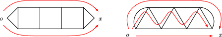
Figure 1: The left figure is an example of the lace-expansion diagrams for percolation, and the right one is for SAW and the Ising model. The number $\ell$ of disjoint paths from $o$ to $x$ using different sets of line segments is 2 in the left figure and 3 in the right figure.

It remains to prove (85)–(LABEL:eq-bnabla-def). By (84), we readily obtain (85) as

$$\qquad\hat{\mathchar 261\relax}_{p}(0)\equiv\sum_{x\in\mathbb{Z}^{d}}\mathchar 261\relax_{p}(x)=1+O\bigl{(}L^{-d}\bigr{)}+O\bigl{(}L^{-d(\ell-1)}\bigr{)}=1+O\bigl{(}L^{-d}\bigr{)}.$$ (92)

Moreover,

$$\bigl{|}\hat{\mathchar 261\relax}_{p}(0)-\hat{\mathchar 261\relax}_{p}(k)\bigr{|}$$

(93)

$$\qquad\equiv\biggl{|}\sum_{x\in\mathbb{Z}^{d}}\bigl{(}1-\cos(k\cdot x)\bigr{)}\mathchar 261\relax_{p}(x)\biggr{|}\leq O\bigl{(}\lambda^{\ell}\bigr{)}\sum_{x\in\mathbb{Z}^{d}}\frac{1-\cos(k\cdot x)}{|\!|\!|x|\!|\!|_{L}^{(d-\alpha\wedge 2)\ell}}.$$

If $\alpha<2$, then there is a $\delta\in(0,(2-\alpha)\wedge((\ell-1)(d-d_{\mathrm{c}})))$ such that $1-\cos(k\cdot x)\leq O(|k\cdot x|^{\alpha+\delta})$, hence

$$\bigl{|}\hat{\mathchar 261\relax}_{p}(0)-\hat{\mathchar 261\relax}_{p}(k)\bigr{|}$$

$$\qquad\leq O\bigl{(}|k|^{\alpha+\delta}\bigr{)}\biggl{(}L^{-d\ell}\sum_{x\dvtx|x|\leq L}|x|^{\alpha+\delta}+L^{-\alpha\ell}\sum_{x\dvtx|x|>L}\frac{|x|^{\alpha+\delta}}{|x|^{(d-\alpha)\ell}}\biggr{)}$$ (94)

$$\qquad=O\bigl{(}L^{-d(\ell-1)+\alpha+\delta}\bigr{)}|k|^{\alpha+\delta}.$$

If $\alpha>2$, then there is a $\delta\in(0,2\wedge((\ell-1)(d-d_{\mathrm{c}})))$ such that $1-\cos(k\cdot x)=\frac{1}{2}|k\cdot x|^{2}+O(|k\cdot x|^{2+\delta})$ and, therefore,

$$\hat{\mathchar 261\relax}_{p}(0)-\hat{\mathchar 261\relax}_{p}(k)$$

$$\qquad=\frac{1}{2}\sum_{x\in\mathbb{Z}^{d}}|k\cdot x|^{2}\mathchar 261\relax_{p}(x)+O\bigl{(}L^{-2\ell}\bigr{)}|k|^{2+\delta}\sum_{x\in\mathbb{Z}^{d}}\frac{|x|^{2+\delta}}{|\!|\!|x|\!|\!|_{L}^{(d-2)\ell}}$$ (95)

$$\qquad=\frac{|k|^{2}}{2d}\sum_{x\in\mathbb{Z}^{d}}|x|^{2}\mathchar 261\relax_{p}(x)+O\bigl{(}L^{-d(\ell-1)+2+\delta}\bigr{)}|k|^{2+\delta}.$$

Then, by the above estimates and (1.1), we obtain

$$\frac{\hat{\mathchar 261\relax}_{p}(0)-\hat{\mathchar 261\relax}_{p}(k)}{1-\hat{D}(k)}$$

(96)

$$\qquad=\cases{O\bigl{(}L^{-d(\ell-1)+\delta}\bigr{)}|k|^{\delta},&\quad$[\alpha<2]$,\vspace*{5pt}\cr\displaystyle\frac{1}{\sigma^{2}}\sum_{x}|x|^{2}\mathchar 261\relax_{p}(x)+O\bigl{(}L^{-d(\ell-1)+\delta}\bigr{)}|k|^{\delta},&\quad$[\alpha>2]$,}$$

hence (LABEL:eq-bnabla-def) by taking $|k|\to 0$. This completes the proof of Proposition 3.1.

Proof of Lemma 3.2 The proof of (87) is almost identical to that of hhs03 , Proposition 1.7(i). However, since we are using $|\!|\!|\cdot|\!|\!|_{L}$ rather than $|\!|\!|\cdot|\!|\!|_{1}$ as in hhs03 , we can gain the extra factor $L^{d-a}$ for $a>d$ in (87). To clarify this, we include the proof here. First of all, since $a\geq b$, we have

$$\sum_{y\in\mathbb{Z}^{d}}|\!|\!|x-y|\!|\!|_{L}^{-a}|\!|\!|y|\!|\!|_{L}^{-b}$$

$$\qquad\leq\sum_{y\dvtx|x-y|\leq|y|}|\!|\!|x-y|\!|\!|_{L}^{-a}|\!|\!|y|\!|\!|_{L}^{-b}+\sum_{y\dvtx|x-y|>|y|}|\!|\!|x-y|\!|\!|_{L}^{-a}|\!|\!|y|\!|\!|_{L}^{-b}$$

$$\qquad\leq 2\sum_{y\dvtx|x-y|\leq|y|}|\!|\!|x-y|\!|\!|_{L}^{-a}|\!|\!|y|\!|\!|_{L}^{-b}.$$

Since $|x-y|\leq|y|$ implies $|y|\geq\frac{1}{2}|x|$, we obtain that, for $a>d$,

$$\sum_{y\dvtx|x-y|\leq|y|}|\!|\!|x-y|\!|\!|_{L}^{-a}|\!|\!|y|\!|\!|_{L}^{-b}$$

$$\qquad\leq 2^{b}|\!|\!|x|\!|\!|_{L}^{-b}\sum_{y\in\mathbb{Z}^{d}}|\!|\!|x-y|\!|\!|_{L}^{-a}$$ (98)

$$\qquad=\frac{C}{2}L^{d-a}|\!|\!|x|\!|\!|_{L}^{-b}.$$

For $a<d$, on the other hand, we use the identity $1={\mathbh 1}_{\{|y|\leq(3/2)|x|\}}+{\mathbh 1}_{\{|y|>(3/2)|x|\}}$ and the fact that $|y|>\frac{3}{2}|x|$ implies $|x-y|\geq\frac{1}{3}|y|$. Then we obtain

$$\sum_{y\dvtx|x-y|\leq|y|}|\!|\!|x-y|\!|\!|_{L}^{-a}|\!|\!|y|\!|\!|_{L}^{-b}$$

$$\qquad\leq 2^{b}|\!|\!|x|\!|\!|_{L}^{-b}\sum_{y\dvtx|x-y|\leq|y|}|\!|\!|x-y|\!|\!|_{L}^{-a}{\mathbh 1}_{\{|y|\leq(3/2)|x|\}}$$

$$\quad\qquad{}+3^{a}\sum_{y\dvtx|x-y|\leq|y|}|\!|\!|y|\!|\!|_{L}^{-a-b}{\mathbh 1}_{\{|y|>(3/2)|x|\}}$$

$$\qquad\leq 2^{b}|\!|\!|x|\!|\!|_{L}^{-b}\sum_{y\dvtx|x-y|\leq(3/2)|x|}|\!|\!|x-y|\!|\!|_{L}^{-a}$$

$$\quad\qquad{}+3^{a}\sum_{y\dvtx|y|>(3/2)|x|}|\!|\!|y|\!|\!|_{L}^{-a-b}$$

$$\qquad\leq\frac{C}{2}|\!|\!|x|\!|\!|_{L}^{d-a-b}.$$

This completes the proof of (87).

The proof of (89) is also quite similar to that of hhs03 , Proposition 1.7(ii), where hhs03 , (5.8), is used. However, hhs03 , (5.8), is valid only for $d>4$, not $d>2$ as claimed in hhs03 , Proposition 1.7(ii). In fact, it is not difficult to avoid this problem, and we include the proof here to clarify this. First, we note that

$$(f*g)(x)=\|g\|_{1}f(x)+\sum_{y\in\mathbb{Z}^{d}}g(y)\bigl{(}f(x-y)-f(x)\bigr{)}.$$ (100)

To prove (89), it suffices to show that the sum in the right-hand side is the error term in (89). For that, we split the sum into the following three sums:

$$\sum_{y\in\mathbb{Z}^{d}} = \sum_{y\dvtx|y|\leq(1/3)|x|}+\sum_{y\dvtx|x-y|\leq(1/3)|x|}+\sum_{y\dvtx|y|\wedge|x-y|>(1/3)|x|}$$

$$\equiv {\sum_{y}}^{\prime}+{\sum_{y}}^{\prime\prime}+{\sum_{y}}^{\prime\prime\prime}.$$

It is not difficult to estimate the last two sums, as

$$\biggl{|}{\sum_{y}}^{\prime\prime}g(y)\bigl{(}f(x-y)-f(x)\bigr{)}\biggr{|}$$

$$\qquad\leq\frac{O(C_{3})}{|\!|\!|x|\!|\!|_{L}^{d+\rho}}\sum_{y\dvtx|x-y|\leq(1/3)|x|}\bigl{(}f(x-y)+f(x)\bigr{)}$$

$$\qquad\leq\frac{O(C_{1}C_{3})}{|\!|\!|x|\!|\!|_{L}^{d-\alpha\wedge 2+\rho}}$$

and

$$\biggl{|}{\sum_{y}}^{\prime\prime\prime}g(y)\bigl{(}f(x-y)-f(x)\bigr{)}\biggr{|}$$

$$\qquad\leq\frac{O(C_{1})}{|\!|\!|x|\!|\!|_{L}^{d-\alpha\wedge 2}}\sum_{y\dvtx|y|>(1/3)|x|}\frac{C_{3}}{|\!|\!|y|\!|\!|_{L}^{d+\rho}}$$ (103)

$$\qquad\leq\frac{O(C_{1}C_{3})}{|\!|\!|x|\!|\!|_{L}^{d-\alpha\wedge 2+\rho}}.$$

To estimate the sum $\sum_{y}^{\prime}$, we use the $\mathbb{Z}^{d}$-symmetry of $g$ to obtain

$${\sum_{y}}^{\prime}g(y)\bigl{(}f(x-y)-f(x)\bigr{)}$$

(104)

$$\qquad=\sum_{y\dvtx 0<|y|\leq(1/3)|x|}g(y)\biggl{(}\frac{f(x+y)+f(x-y)}{2}-f(x)\biggr{)}.$$

Notice that

$$\biggl{|}\frac{f(x+y)+f(x-y)}{2}-f(x)\biggr{|}$$

(105)

$$\qquad\leq\frac{O(C_{1})}{|\!|\!|x|\!|\!|_{L}^{d-\alpha\wedge 2}}\times\cases{1,&\quad$\biggl{[}|x|\leq\dfrac{3}2L\biggr{]}$,\vspace*{5pt}\cr|y|^{2}/|x|^{2},&\quad$\biggl{[}|x|\geq\dfrac{3}2L\biggr{]}$.}$$

To verify this for $|x|\leq\frac{3}{2}L$, we simply bound each $f$ by $O(C_{1})|\!|\!|x|\!|\!|_{L}^{\alpha\wedge 2-d}$. For $|x|\geq\frac{3}{2}L$, since $|x\pm y|\geq|x|-|y|\geq\frac{2}{3}|x|\geq L$, we have $f(x\pm y)=C_{1}|x\pm y|^{\alpha\wedge 2-d}$. Then, by Taylor’s theorem, since $|{\pm}2\frac{x\cdot y}{|x|^{2}}+\frac{|y|^{4}}{|x|^{4}}|\leq\frac{7}{9}<1$, we have

$$|x\pm y|^{\alpha\wedge 2-d} = |x|^{\alpha\wedge 2-d}\biggl{(}1\pm 2\frac{x\cdot y}{|x|^{2}}+\frac{|y|^{4}}{|x|^{4}}\biggr{)}^{(\alpha\wedge 2-d)/2}$$

$$= |x|^{\alpha\wedge 2-d}\biggl{(}1\mp(d-\alpha\wedge 2)\frac{x\cdot y}{|x|^{2}}+O\biggl{(}\frac{|y|^{2}}{|x|^{2}}\biggr{)}\biggr{)}$$

and (3.1) follows. Therefore, if $|x|\leq\frac{3}{2}L$, then $|y|\leq\frac{1}{2}L$ and we obtain

$$\qquad\biggl{|}{\sum_{y}}^{\prime}g(y)\bigl{(}f(x-y)-f(x)\bigr{)}\biggr{|} \leq \frac{O(C_{1})}{|\!|\!|x|\!|\!|_{L}^{d-\alpha\wedge 2}}\sum_{y\dvtx 0<|y|\leq(1/2)L}\frac{C_{3}}{L^{d+\rho}}$$

$$\leq \frac{O(C_{1}C_{3})}{|\!|\!|x|\!|\!|_{L}^{d-\alpha\wedge 2+\rho}}.$$

If $|x|\geq\frac{3}{2}L$, then $|\!|\!|x|\!|\!|_{L}=|x|$ and we obtain

$$\biggl{|}{\sum_{y}}^{\prime}g(y)\bigl{(}f(x-y)-f(x)\bigr{)}\biggr{|}$$

$$\qquad\leq\frac{O(C_{1})}{|\!|\!|x|\!|\!|_{L}^{d-\alpha\wedge 2+2}}\sum_{y\dvtx 0<|y|\leq(1/3)|x|}|y|^{2}\biggl{(}\frac{C_{3}{\mathbh 1}_{\{|y|\leq L\}}}{L^{d+\rho}}+\frac{C_{3}{\mathbh 1}_{\{|y|>L\}}}{|y|^{d+\rho}}\biggr{)}$$

$$\qquad\leq\frac{O(C_{1}C_{3})}{|\!|\!|x|\!|\!|_{L}^{d-\alpha\wedge 2+2}}\times\cases{L^{-\rho+2},&\quad$[\rho>2]$,\vspace*{2pt}\cr\log|x|,&\quad$[\rho=2]$,\vspace*{2pt}\cr|x|^{2-\rho},&\quad$[\rho<2]$.}$$

Summarizing the above yields (89). This completes the proof of Lemma 3.2.

3.2 Proof of the infrared bound on $G_{p}$

In this subsection, we prove that the hypothesis of Proposition 3.1 indeed holds for $p\leq p_{\mathrm{c}}$ in high dimensions. The precise statement is the following.

Theorem 3.3

Let $\alpha>0$, $\alpha\neq 2$ and $d>d_{\mathrm{c}}$, and assume the properties (16), (1.1) and (1.2) in Assumption 1.1. Then, for $L\gg 1$ and $p\leq p_{\mathrm{c}}$,

$$G_{p}(x)\leq O\bigl{(}L^{-\alpha\wedge 2}\bigr{)}|\!|\!|x|\!|\!|_{L}^{\alpha\wedge 2-d}\qquad[x\neq o].$$ (109)

Let

$$g_{p}=p\vee\sup_{x\neq o}\frac{G_{p}(x)}{\lambda|\!|\!|x|\!|\!|_{L}^{\alpha\wedge 2-d}},$$ (110)

where we recall the definition (81) of $\lambda$. Suppose that the following properties hold: [(iii)]

$g_{p}$ is continuous (and nondecreasing) in $p\in[1,p_{\mathrm{c}})$.

$g_{1}\leq 1$.

If $\lambda\ll 1$ (i.e., $L\gg 1$), then $g_{p}\leq 3$ implies $g_{p}\leq 2$ for every $p\in(1,p_{\mathrm{c}})$. If the above properties hold, then in fact $g_{p}\leq 2$ for all $p<p_{\mathrm{c}}$, as long as $d>d_{\mathrm{c}}$ and $\lambda\ll 1$. In particular, $G_{p}(x)\leq 2\lambda|\!|\!|x|\!|\!|_{L}^{\alpha\wedge 2-d}$ for all $x\neq o$ and $p<p_{\mathrm{c}}$ $(\leq 2)$. By Lemma 2.2, we can extend this bound up to $p=p_{\mathrm{c}}$, hence the proof completed.

Now we verify those properties (i)–(iii).

Verification of (i). It suffices to show that, for every $p_{0}\in(1,p_{\mathrm{c}})$,$\sup_{x\neq o}G_{p}(x)/|\!|\!|x|\!|\!|_{L}^{\alpha\wedge 2-d}$ is continuous in $p\in[1,p_{0}]$. By the monotonicity of $G_{p}(x)$ in $p\leq p_{0}$ and using Lemma 2.4, we have

$$\frac{G_{p}(x)}{|\!|\!|x|\!|\!|_{L}^{\alpha\wedge 2-d}}\leq\frac{G_{p_{0}}(x)}{|\!|\!|x|\!|\!|_{L}^{\alpha\wedge 2-d}}\leq\frac{K_{p_{0}}|\!|\!|x|\!|\!|_{L}^{-d-\alpha}}{|\!|\!|x|\!|\!|_{L}^{\alpha\wedge 2-d}}=\frac{K_{p_{0}}}{|\!|\!|x|\!|\!|_{L}^{\alpha+\alpha\wedge 2}}.$$ (111)

On the other hand, for any $x_{0}\neq o$ with $D(x_{0})>0$, there exists an $R=R(p_{0},x_{0})<\infty$ such that, for all $|x|\geq R$,

$$\frac{K_{p_{0}}}{|\!|\!|x|\!|\!|_{L}^{\alpha+\alpha\wedge 2}}\leq\frac{D(x_{0})}{|\!|\!|x_{0}|\!|\!|_{L}^{\alpha\wedge 2-d}}.$$ (112)

Moreover, by using $p\geq 1$ and the lower bound of the second inequality in (59), we have

$$\frac{D(x_{0})}{|\!|\!|x_{0}|\!|\!|_{L}^{\alpha\wedge 2-d}}\leq\frac{pD(x_{0})}{|\!|\!|x_{0}|\!|\!|_{L}^{\alpha\wedge 2-d}}\leq\frac{G_{p}(x_{0})}{|\!|\!|x_{0}|\!|\!|_{L}^{\alpha\wedge 2-d}}.$$ (113)

As a result, for any $p\in[1,p_{0}]$, we obtain

$$\sup_{x\neq o}\frac{G_{p}(x)}{|\!|\!|x|\!|\!|_{L}^{\alpha\wedge 2-d}}=\frac{G_{p}(x_{0})}{|\!|\!|x_{0}|\!|\!|_{L}^{\alpha\wedge 2-d}}\vee\max_{x\dvtx 0<|x|<R}\frac{G_{p}(x)}{|\!|\!|x|\!|\!|_{L}^{\alpha\wedge 2-d}}.$$ (114)

Since $G_{p}(x)$ is continuous in $p$ (cf., Lemma 2.2) and the maximum of finitely many continuous functions is continuous, we can conclude that $g_{p}$ is continuous in $p\in[1,p_{0}]$, as required.

Verification of (ii). By the first inequality in (59) and the definition (81) of $\lambda$, we readily obtain

$$g_{1}=1\vee\sup_{x\neq o}\frac{G_{1}(x)}{\lambda|\!|\!|x|\!|\!|_{L}^{\alpha\wedge 2-d}}\leq 1\vee\sup_{x\neq o}\frac{S_{1}(x)}{\lambda|\!|\!|x|\!|\!|_{L}^{\alpha\wedge 2-d}}=1$$ (115)

as required.

Verification of (iii). If $d>d_{\mathrm{c}}$, $\lambda\ll 1$ and $g_{p}\leq 3$, then, by Proposition 3.1, $\mathchar 261\relax_{p}$ satisfies (84)–(LABEL:eq-bnabla-def) as well as (3.1). We use these estimates and the lace expansion to prove $g_{p}\leq 2$ as follows.

First, we recall (12) and (32):

$$G_{p}=\mathchar 261\relax_{p}+\mathchar 261\relax_{p}*pD*G_{p},\qquad S_{p}=\delta+pD*S_{p},$$ (116)

or equivalently

$$\mathchar 261\relax_{p}=G_{p}*(\delta-\mathchar 261\relax_{p}*pD),\qquad\delta=(\delta-pD)*S_{p}.$$ (117)

Inspired by the similarity of the above identities, we approximate $G_{p}$ to $r\mathchar 261\relax_{p}*S_{q}$ with some constant $r\in(0,\infty)$ and the parameter change $q\in[0,1]$. Rewrite $G_{p}$ as follows:

$$\qquad G_{p} = r\mathchar 261\relax_{p}*S_{q}+G_{p}*\delta-r\mathchar 261\relax_{p}*S_{q}$$

$$= r\mathchar 261\relax_{p}*S_{q}+G_{p}*(\delta-qD)*S_{q}-rG_{p}*(\delta-\mathchar 261\relax_{p}*pD)*S_{q}$$

$$= r\mathchar 261\relax_{p}*S_{q}+G_{p}*E_{p,q,r}*S_{q},\$$

where

$$E_{p,q,r}=\delta-qD-r(\delta-\mathchar 261\relax_{p}*pD).$$ (119)

We choose $q,r$ to satisfy

$$\hat{E}_{p,q,r}(0)=\bar{\nabla}^{\alpha\wedge 2}\hat{E}_{p,q,r}(0)=0,$$ (120)

or equivalently

$$\cases{1-q-r\bigl{(}1-\hat{\mathchar 261\relax}_{p}(0)p\bigr{)}=0,\vspace*{4pt}\cr-q+r\bigl{(}\hat{\mathchar 261\relax}_{p}(0)+\bar{\nabla}^{\alpha\wedge 2}\hat{\mathchar 261\relax}_{p}(0)\bigr{)}p=0.}$$ (121)

Solving these simultaneous equations for $r$ and using (LABEL:eq-bnabla-def), we obtain

$$r=\bigl{(}1+p\bar{\nabla}^{\alpha\wedge 2}\hat{\mathchar 261\relax}_{p}(0)\bigr{)}^{-1}=1+\cases{0,&\quad$[\alpha<2]$,\vspace*{2pt}\cr O\bigl{(}L^{-d(\ell-1)}\bigr{)},&\quad$[\alpha>2]$.}$$ (122)

On the other hand, by taking the Fourier transform of (116) and setting $k=0$, we obtain

$$\chi_{p}=\hat{\mathchar 261\relax}_{p}(0)+\hat{\mathchar 261\relax}_{p}(0)p\chi_{p},$$ (123)

or equivalently $\hat{\mathchar 261\relax}_{p}(0)=\chi_{p}/(1+p\chi_{p})$ and, therefore,

$$q=1-r\bigl{(}1-\hat{\mathchar 261\relax}_{p}(0)p\bigr{)}=1-\frac{r}{1+p\chi_{p}}\in(0,1],$$ (124)

where we have used $p\geq 1$, $\chi_{p}\geq 1$ and (122) to guarantee the positivity (by taking $L\gg 1$ if $\alpha>2$).

In addition, by solving (123) for $\chi_{p}$ and using (85), we have

$$\chi_{p}=\frac{\hat{\mathchar 261\relax}_{p}(0)}{1-\hat{\mathchar 261\relax}_{p}(0)p}=\frac{1+O(L^{-d})}{1-\hat{\mathchar 261\relax}_{p}(0)p},$$ (125)

hence $1-\hat{\mathchar 261\relax}_{p}(0)p\geq 0$. In particular, $p\leq\hat{\mathchar 261\relax}_{p}(0)^{-1}=1+O(L^{-d})\leq 2$, as required.

It remains to prove $G_{p}(x)\leq 2\lambda|\!|\!|x|\!|\!|_{L}^{\alpha\wedge 2-d}$. To do so, we use the following property of $E_{p,q,r}$.

Proposition 3.4.

Let $q,r$ be defined as in (122)–(124). Under the hypothesis of Proposition 3.1, there is a $\rho\in(0,\alpha\wedge 2)$ such that

$$\bigl{|}(E_{p,q,r}*S_{q})(x)\bigr{|}\leq O\bigl{(}L^{-d(\ell-1)}\bigr{)}\biggl{(}{\mathbh 1}_{\{\alpha>2\}}\delta_{o,x}+\frac{L^{\rho}}{|\!|\!|x|\!|\!|_{L}^{d+\rho}}\biggr{)}.$$ (126)

For now, we assume this proposition and complete verifying the property (iii). First, by rearranging (3.2) and using $S_{q}\leq S_{1}$ as well as (85) and (122) for $L\gg 1$, we obtain

$$\qquad G_{p} = r\mathchar 261\relax_{p}*S_{q}+G_{p}*E_{p,q,r}*S_{q}$$

$$= r\hat{\mathchar 261\relax}_{p}(0)S_{q}-r\bigl{(}\hat{\mathchar 261\relax}_{p}(0)\delta-\mathchar 261\relax_{p}\bigr{)}*S_{q}+G_{p}*E_{p,q,r}*S_{q}$$

$$\leq \bigl{(}1+O\bigl{(}L^{-d}\bigr{)}\bigr{)}S_{1}-r\bigl{(}\hat{\mathchar 261\relax}_{p}(0)\delta-\mathchar 261\relax_{p}\bigr{)}*S_{q}+G_{p}*E_{p,q,r}*S_{q}.$$

Then, by Proposition 3.4 and Lemma 3.2(i), the third term is bounded as

$$\bigl{|}(G_{p}*E_{p,q,r}*S_{q})(x)\bigr{|}$$

$$\qquad\leq O\bigl{(}L^{-d(\ell-1)}\bigr{)}\sum_{y\in\mathbb{Z}^{d}}\frac{3\lambda}{|\!|\!|y|\!|\!|_{L}^{d-\alpha\wedge 2}}\biggl{(}\delta_{y,x}+\frac{L^{\rho}}{|\!|\!|x-y|\!|\!|_{L}^{d+\rho}}\biggr{)}$$ (128)

$$\qquad\leq\frac{O(L^{-d(\ell-1)})\lambda}{|\!|\!|x|\!|\!|_{L}^{d-\alpha\wedge 2}}.$$

Also, by (84) and Lemma 3.2(i), the second term in (3.2) is bounded as

$$\bigl{|}\bigl{(}\bigl{(}\hat{\mathchar 261\relax}_{p}(0)\delta-\mathchar 261\relax_{p}\bigr{)}*S_{q}\bigr{)}(x)\bigr{|}$$

$$\qquad=\biggl{|}\sum_{y\neq o}\mathchar 261\relax_{p}(y)\bigl{(}S_{q}(x)-S_{q}(x-y)\bigr{)}\biggr{|}$$

(129)

$$\qquad\leq\sum_{y\neq o}\bigl{|}\mathchar 261\relax_{p}(y)\bigr{|}S_{q}(x)+\sum_{y\neq o}\bigl{|}\mathchar 261\relax_{p}(y)\bigr{|}S_{q}(x-y)$$

$$\qquad\leq\frac{O(L^{-d(\ell-1)})\lambda}{|\!|\!|x|\!|\!|_{L}^{d-\alpha\wedge 2}}.$$

Putting these estimates back into (3.2), we obtain that, for $L\gg 1$,

$$\qquad G_{p}(x)\leq\bigl{(}1+O\bigl{(}L^{-d}\bigr{)}\bigr{)}\frac{\lambda}{|\!|\!|x|\!|\!|_{L}^{d-\alpha\wedge 2}}+\frac{O(L^{-d(\ell-1)})\lambda}{|\!|\!|x|\!|\!|_{L}^{d-\alpha\wedge 2}}\leq\frac{2\lambda}{|\!|\!|x|\!|\!|_{L}^{d-\alpha\wedge 2}}$$ (130)

as required. This completes the proof of Theorem 3.3 assuming Proposition 3.4.

Proof of Proposition 3.4 First, by substituting $q=1-r(1-\hat{\mathchar 261\relax}_{p}(0)p)$ [cf., (124)] into (119) and using $1-r=pr\bar{\nabla}^{\alpha\wedge 2}\hat{\mathchar 261\relax}_{p}(0)$ [cf., (122)], we obtain

$$E_{p,q,r}=pr\bigl{(}\bar{\nabla}^{\alpha\wedge 2}\hat{\mathchar 261\relax}_{p}(0)(\delta-D)-\bigl{(}\hat{\mathchar 261\relax}_{p}(0)\delta-\mathchar 261\relax_{p}\bigr{)}*D\bigr{)}.$$ (131)

Using this representation, we prove (126) for $|x|\leq 2L$ and $|x|>2L$, separately.

For $|x|\leq 2L$, we simply use (35) to bound $|(E_{p,q,r}*S_{q})(x)|$ by

$$\bigl{|}(E_{p,q,r}*S_{q})(x)\bigr{|}\leq\bigl{|}E_{p,q,r}(x)\bigr{|}+O\bigl{(}L^{-d}\bigr{)}\sum_{y\in\mathbb{Z}^{d}}\bigl{|}E_{p,q,r}(y)\bigr{|}.$$ (132)

By (131), we have

$$\frac{|E_{p,q,r}(x)|}{pr}$$

$$\qquad\leq\bigl{|}\bar{\nabla}^{\alpha\wedge 2}\hat{\mathchar 261\relax}_{p}(0)\bigr{|}\bigl{(}\delta_{o,x}+D(x)\bigr{)}+\bigl{|}\bigl{(}\bigl{(}\hat{\mathchar 261\relax}_{p}(0)\delta-\mathchar 261\relax_{p}\bigr{)}*D\bigr{)}(x)\bigr{|}$$

$$\qquad=\bigl{|}\bar{\nabla}^{\alpha\wedge 2}\hat{\mathchar 261\relax}_{p}(0)\bigr{|}\bigl{(}\delta_{o,x}+D(x)\bigr{)}+\biggl{|}\sum_{z\neq o}\mathchar 261\relax_{p}(z)\bigl{(}D(x)-D(x-z)\bigr{)}\biggr{|}$$

$$\qquad\leq\bigl{|}\bar{\nabla}^{\alpha\wedge 2}\hat{\mathchar 261\relax}_{p}(0)\bigr{|}\bigl{(}\delta_{o,x}+D(x)\bigr{)}+\sum_{z\neq o}\bigl{|}\mathchar 261\relax_{p}(z)\bigr{|}\bigl{(}D(x)+D(x-z)\bigr{)}.$$

Using (84)–(LABEL:eq-bnabla-def) and (122), we obtain that

$$\bigl{|}E_{p,q,r}(x)\bigr{|}$$

$$\qquad\leq O\bigl{(}L^{-d(\ell-1)}\bigr{)}{\mathbh 1}_{\{\alpha>2\}}\bigl{(}\delta_{o,x}+O\bigl{(}L^{-d}\bigr{)}\bigr{)}+O\bigl{(}L^{-d}\bigr{)}\sum_{z\neq o}\bigl{|}\mathchar 261\relax_{p}(z)\bigr{|}$$ (134)

$$\qquad\leq O\bigl{(}L^{-d(\ell-1)}\bigr{)}{\mathbh 1}_{\{\alpha>2\}}\delta_{o,x}+O\bigl{(}L^{-d\ell}\bigr{)}$$

and that, by summing (3.2) over $x\in\mathbb{Z}^{d}$,

$$O\bigl{(}L^{-d}\bigr{)}\sum_{x\in\mathbb{Z}^{d}}\bigl{|}E_{p,q,r}(x)\bigr{|}$$

$$\qquad\leq O\bigl{(}L^{-d}\bigr{)}\biggl{(}2\bigl{|}\bar{\nabla}^{\alpha\wedge 2}\hat{\mathchar 261\relax}_{p}(0)\bigr{|}+2\sum_{z\neq o}\bigl{|}\mathchar 261\relax_{p}(z)\bigr{|}\biggr{)}$$ (135)

$$\qquad\leq O\bigl{(}L^{-d\ell}\bigr{)}.$$

Therefore, for $|x|\leq 2L$,

$$\bigl{|}(E_{p,q,r}*S_{q})(x)\bigr{|} \leq O\bigl{(}L^{-d(\ell-1)}\bigr{)}{\mathbh 1}_{\{\alpha>2\}}\delta_{o,x}+O\bigl{(}L^{-d\ell}\bigr{)}$$

$$\leq O\bigl{(}L^{-d(\ell-1)}\bigr{)}{\mathbh 1}_{\{\alpha>2\}}\delta_{o,x}+\frac{O(L^{-d(\ell-1)+\rho})}{|\!|\!|x|\!|\!|_{L}^{d+\rho}}.$$

It remains to prove (126) for $|x|>2L$. To do so, we first rewrite $(E_{p,q,r}*S_{q})(x)$ as

$$\qquad(E_{p,q,r}*S_{q})(x) = \int_{[-\pi,\pi]^{d}}\frac{\mathrm{d}^{d}k}{(2\pi)^{d}}\hat{E}_{p,q,r}(k)\frac{e^{-ik\cdot x}}{1-q\hat{D}(k)}$$

$$= \int_{0}^{\infty}\mathrm{d}t\int_{[-\pi,\pi]^{d}}\frac{\mathrm{d}^{d}k}{(2\pi)^{d}}\hat{E}_{p,q,r}(k)e^{-t(1-q\hat{D}(k))-ik\cdot x}.$$

Then we split the integral with respect to $t$ into $\int_{0}^{T}$ and $\int_{T}^{\infty}$, where $T$ is arbitrary for now, but it will be determined shortly. For the latter integral, we use the Fourier transform of (131), which is

$$\qquad\hat{E}_{p,q,r}(k)=pr\bigl{(}1-\hat{D}(k)\bigr{)}\biggl{(}\bar{\nabla}^{\alpha\wedge 2}\hat{\mathchar 261\relax}_{p}(0)-\frac{\hat{\mathchar 261\relax}_{p}(0)-\hat{\mathchar 261\relax}_{p}(k)}{1-\hat{D}(k)}\hat{D}(k)\biggr{)}.$$ (138)

Because of (1.1), (LABEL:eq-bnabla-def) and (3.1), there is a $\delta>0$ such that

$$\hat{E}_{p,q,r}(k)=O\bigl{(}L^{-d(\ell-1)+\alpha\wedge 2+\delta}\bigr{)}|k|^{\alpha\wedge 2+\delta}\qquad[\alpha\neq 2].$$ (139)

Since $1-q\hat{D}(k)\geq q(1-\hat{D}(k))$, the contribution to (3.2) from the large-$t$ integral is bounded as

$$\biggl{|}\int_{T}^{\infty}\mathrm{d}t\int_{[-\pi,\pi]^{d}}\frac{\mathrm{d}^{d}k}{(2\pi)^{d}}\hat{E}_{p,q,r}(k)e^{-t(1-q\hat{D}(k))-ik\cdot x}\biggr{|}$$

(140)

$$\qquad\leq O\bigl{(}L^{-d(\ell-1)+\alpha\wedge 2+\delta}\bigr{)}\int_{T}^{\infty}\mathrm{d}t\int_{[-\pi,\pi]^{d}}\frac{\mathrm{d}^{d}k}{(2\pi)^{d}}|k|^{\alpha\wedge 2+\delta}e^{-tq(1-\hat{D}(k))}.$$

Since $p\geq 1$, we have $q\geq 1-r/(1+\chi_{1})\geq 1-r/2$ [cf., (124)], which is bounded away from zero when $L\gg 1$. Therefore, by using (1.1), we obtain

$$\qquad\int_{[-\pi,\pi]^{d}}\frac{\mathrm{d}^{d}k}{(2\pi)^{d}}|k|^{\alpha\wedge 2+\delta}e^{-tq(1-\hat{D}(k))}=O\bigl{(}L^{\alpha\wedge 2}t\bigr{)}^{-1-((d+\delta)/(\alpha\wedge 2))},$$ (141)

hence

$$\biggl{|}\int_{T}^{\infty}\mathrm{d}t\int_{[-\pi,\pi]^{d}}\frac{\mathrm{d}^{d}k}{(2\pi)^{d}}\hat{E}_{p,q,r}(k)e^{-t(1-q\hat{D}(k))-ik\cdot x}\biggr{|}$$

(142)

$$\qquad\leq O\bigl{(}L^{-d\ell}\bigr{)}T^{-(d+\delta)/(\alpha\wedge 2)}.$$

Let

$$\rho=\frac{(\alpha\wedge 2)\delta}{d+\alpha\wedge 2+\delta},\qquad T=\biggl{(}\frac{|x|}{L}\biggr{)}^{\alpha\wedge 2-\rho}.$$ (143)

Then, since $|x|>2L$,

$$O\bigl{(}L^{-d\ell}\bigr{)}T^{-(d+\delta)/(\alpha\wedge 2)}=\frac{O(L^{-d(\ell-1)+\rho})}{|\!|\!|x|\!|\!|_{L}^{d+\rho}}.$$ (144)

To estimate the contribution to (3.2) from the small-$t$ integral, we use the identity

$$\int_{0}^{T}\mathrm{d}t\int_{[-\pi,\pi]^{d}}\frac{\mathrm{d}^{d}k}{(2\pi)^{d}}\hat{E}_{p,q,r}(k)e^{-t(1-q\hat{D}(k))-ik\cdot x}$$

(145)

$$\qquad=\int_{0}^{T}\mathrm{d}t\,e^{-t}\sum_{n=0}^{\infty}\frac{(tq)^{n}}{n!}\bigl{(}E_{p,q,r}*D^{*n}\bigr{)}(x),$$

where, by (131) and (LABEL:eq-bnabla-def),

$$\bigl{(}E_{p,q,r}*D^{*n}\bigr{)}(x) = \underbrace{pr\bar{\nabla}^{\alpha\wedge 2}\hat{\mathchar 261\relax}_{p}(0)}_{O(L^{-d(\ell-1)}){\mathbh 1}_{\{\alpha>2\}}}\sum_{y\in\mathbb{Z}^{d}}D(y)\bigl{(}D^{*n}(x)-D^{*n}(x-y)\bigr{)}$$

$${}-pr\sum_{y\in\mathbb{Z}^{d}}\mathchar 261\relax_{p}(y)\bigl{(}D^{*(n+1)}(x)-D^{*(n+1)}(x-y)\bigr{)}.$$

In the following, we use the decomposition (3.1) of $\sum_{y}$ and estimate the contribution to (3.2) from $\sum_{y}^{\prime}$, $\sum_{y}^{\prime\prime}$ and $\sum_{y}^{\prime\prime\prime}$, separately.

First, we estimate the contribution from $\sum_{y}^{\prime\prime}\equiv\sum_{y\dvtx|x-y|\leq(1/3)|x|}$. Since $|y|\geq|x|-|x-y|\geq\frac{2}{3}|x|$ in this domain of summation, we bound $|\mathchar 261\relax_{p}(y)|$ by $O(\lambda^{\ell})|\!|\!|x|\!|\!|_{L}^{(\alpha\wedge 2-d)\ell}$ [cf., (84)] and then use (21), $\sum_{y}^{\prime\prime}1\leq O(|\!|\!|x|\!|\!|_{L}^{d})$ and $\sum_{y}^{\prime\prime}D^{*(n+1)}(x-y)\leq 1$. As a result,

$$\biggl{|}{\sum_{y}}^{\prime\prime}\mathchar 261\relax_{p}(y)\bigl{(}D^{*(n+1)}(x)-D^{*(n+1)}(x-y)\bigr{)}\biggr{|}$$

$$\qquad\leq\frac{O(\lambda^{\ell})}{|\!|\!|x|\!|\!|_{L}^{(d-\alpha\wedge 2)\ell}}\biggl{(}\frac{O(L^{\alpha\wedge 2})n}{|\!|\!|x|\!|\!|_{L}^{\alpha\wedge 2}}+1\biggr{)}$$ (147)

$$\qquad\leq\frac{O(L^{-d(\ell-1)+\alpha\wedge 2})}{|\!|\!|x|\!|\!|_{L}^{d+\alpha\wedge 2}}\biggl{(}\frac{O(L^{\alpha\wedge 2})n}{|\!|\!|x|\!|\!|_{L}^{\alpha\wedge 2}}+1\biggr{)}.$$

Similarly, for $\alpha>2$,

$$O\bigl{(}L^{-d(\ell-1)}\bigr{)}\biggl{|}{\sum_{y}}^{\prime\prime}D(y)\bigl{(}D^{*n}(x)-D^{*n}(x-y)\bigr{)}\biggr{|}$$

$$\qquad\leq\frac{O(L^{-d(\ell-1)+\alpha})}{|\!|\!|x|\!|\!|_{L}^{d+\alpha}}\biggl{(}\frac{O(L^{2})n}{|\!|\!|x|\!|\!|_{L}^{2}}+1\biggr{)}$$ (148)

$$\qquad\leq\frac{O(L^{-d(\ell-1)+2})}{|\!|\!|x|\!|\!|_{L}^{d+2}}\biggl{(}\frac{O(L^{2})n}{|\!|\!|x|\!|\!|_{L}^{2}}+1\biggr{)}.$$

To estimate the contribution to (3.2) from $\sum_{y}^{\prime\prime\prime}\equiv\sum_{y\dvtx|y|\wedge|x-y|>(1/3)|x|}$ in (3.2), we bound $D^{*(n+1)}(x)$ and $D^{*(n+1)}(x-y)$ by $O(L^{\alpha\wedge 2})n/|\!|\!|x|\!|\!|_{L}^{d+\alpha\wedge 2}$ and then use (84) to bound $|\mathchar 261\relax_{p}(y)|$. The result is

$$\biggl{|}{\sum_{y}}^{\prime\prime\prime}\mathchar 261\relax_{p}(y)\bigl{(}D^{*(n+1)}(x)-D^{*(n+1)}(x-y)\bigr{)}\biggr{|}$$

$$\qquad\leq\frac{O(L^{\alpha\wedge 2})n}{|\!|\!|x|\!|\!|_{L}^{d+\alpha\wedge 2}}\sum_{y\dvtx|y|>(1/3)|x|}\bigl{|}\mathchar 261\relax_{p}(y)\bigr{|}$$ (149)

$$\qquad\leq\frac{O(L^{-(\ell-1)(\alpha\wedge 2)})n}{|\!|\!|x|\!|\!|_{L}^{d+2(\alpha\wedge 2)+(\ell-1)(d-d_{\mathrm{c}})}}\leq\frac{O(L^{-d(\ell-1)+2(\alpha\wedge 2)})n}{|\!|\!|x|\!|\!|_{L}^{d+2(\alpha\wedge 2)}}.$$

Similarly, for $\alpha>2$,

$$O\bigl{(}L^{-d(\ell-1)}\bigr{)}\biggl{|}{\sum_{y}}^{\prime\prime\prime}D(y)\bigl{(}D^{*n}(x)-D^{*n}(x-y)\bigr{)}\biggr{|}$$

$$\qquad\leq\frac{O(L^{-d(\ell-1)+2})n}{|\!|\!|x|\!|\!|_{L}^{d+2}}\sum_{y\dvtx|y|>(1/3)|x|}D(y)$$ (150)

$$\qquad\leq\frac{O(L^{-d(\ell-1)+4})n}{|\!|\!|x|\!|\!|_{L}^{d+4}}.$$

Finally, we estimate the contribution to (3.2) from $\sum_{y}^{\prime}\equiv\sum_{y\dvtx|y|\leq(1/3)|x|}$ in (3.2). By the $\mathbb{Z}^{d}$-symmetry of $\mathchar 261\relax_{p}$ and using (84) and the assumption (1.2), we obtain

$$\biggl{|}{\sum_{y}}^{\prime}\mathchar 261\relax_{p}(y)\bigl{(}D^{*(n+1)}(x)-D^{*(n+1)}(x-y)\bigr{)}\biggr{|}$$

$$\qquad=\biggl{|}{\sum_{y}}^{\prime}\mathchar 261\relax_{p}(y)\biggl{(}D^{*(n+1)}(x)-\frac{D^{*(n+1)}(x+y)+D^{*(n+1)}(x-y)}{2}\biggr{)}\biggr{|}$$

$$\qquad\leq\frac{O(L^{\alpha\wedge 2})n}{|\!|\!|x|\!|\!|_{L}^{d+\alpha\wedge 2+2}}\sum_{y\dvtx|y|\leq(1/3)|x|}\frac{O(\lambda^{\ell})|\!|\!|y|\!|\!|_{L}^{2}}{|\!|\!|y|\!|\!|_{L}^{(d-\alpha\wedge 2)\ell}}$$

$$\qquad\leq\frac{O(L^{-(\ell-1)(\alpha\wedge 2)})n}{|\!|\!|x|\!|\!|_{L}^{d+\alpha\wedge 2+2}}$$

$$\quad\qquad{}\times\cases{|\!|\!|x|\!|\!|_{L}^{d+2-(d-\alpha\wedge 2)\ell},&\quad$\bigl{[}d+2>(d-\alpha\wedge 2)\ell\bigr{]}$,\vspace*{4pt}\cr 1+\log\bigl{(}|\!|\!|x|\!|\!|_{L}/L\bigr{)},&\quad$\bigl{[}d+2=(d-\alpha\wedge 2)\ell\bigr{]}$,\vspace*{4pt}\cr L^{d+2-(d-\alpha\wedge 2)\ell},&\quad$\bigl{[}d+2<(d-\alpha\wedge 2)\ell\bigr{]}$,}$$

$$\qquad\leq\frac{O(L^{-d(\ell-1)+2(\alpha\wedge 2)})n}{|\!|\!|x|\!|\!|_{L}^{d+2(\alpha\wedge 2)}},$$

where, to obtain the last inequality for $d+2=(d-\alpha\wedge 2)\ell$, which implies $\alpha<2$, we have used fact that $(|\!|\!|x|\!|\!|_{L}/L)^{\alpha-2}(1+\log(|\!|\!|x|\!|\!|_{L}/L))$ is bounded. Similarly, for $\alpha>2$,

$$O\bigl{(}L^{-d(\ell-1)}\bigr{)}\biggl{|}{\sum_{y}}^{\prime}D(y)\bigl{(}D^{*n}(x)-D^{*n}(x-y)\bigr{)}\biggr{|}$$

$$\qquad=O\bigl{(}L^{-d(\ell-1)}\bigr{)}\biggl{|}{\sum_{y}}^{\prime}D(y)\biggl{(}D^{*n}(x)-\frac{D^{*n}(x+y)+D^{*n}(x-y)}{2}\biggr{)}\biggr{|}$$

$$\qquad\leq\frac{O(L^{-d(\ell-1)+2})n}{|\!|\!|x|\!|\!|_{L}^{d+4}}\underbrace{\sum_{y\dvtx|y|\leq(1/3)|x|}\frac{O(L^{\alpha})|\!|\!|y|\!|\!|_{L}^{2}}{|\!|\!|y|\!|\!|_{L}^{d+\alpha}}}_{O(L^{2})}$$

$$\qquad=\frac{O(L^{-d(\ell-1)+4})n}{|\!|\!|x|\!|\!|_{L}^{d+4}}.$$

Now, by putting these estimates back into (3.2), we obtain

$$\bigl{|}\bigl{(}E_{p,q,r}*D^{*n}\bigr{)}(x)\bigr{|}\leq\frac{O(L^{-d(\ell-1)+\alpha\wedge 2})}{|\!|\!|x|\!|\!|_{L}^{d+\alpha\wedge 2}}\biggl{(}\frac{O(L^{\alpha\wedge 2})}{|\!|\!|x|\!|\!|_{L}^{\alpha\wedge 2}}n+1\biggr{)},$$ (153)

hence, by (143),

$$\Biggl{|}\int_{0}^{T}\mathrm{d}t\,e^{-t}\sum_{n=0}^{\infty}\frac{(tq)^{n}}{n!}\bigl{(}E_{p,q,r}*D^{*n}\bigr{)}(x)\Biggr{|}$$

$$\qquad\leq\frac{O(L^{-d(\ell-1)+\alpha\wedge 2})}{|\!|\!|x|\!|\!|_{L}^{d+\alpha\wedge 2}}\biggl{(}\frac{O(L^{\alpha\wedge 2})}{|\!|\!|x|\!|\!|_{L}^{\alpha\wedge 2}}T^{2}+T\biggr{)}$$ (154)

$$\qquad\leq\frac{O(L^{-d(\ell-1)+\alpha\wedge 2})}{|\!|\!|x|\!|\!|_{L}^{d+\alpha\wedge 2}}T=\frac{O(L^{-d(\ell-1)+\rho})}{|\!|\!|x|\!|\!|_{L}^{d+\rho}}.$$

This completes the proof of Proposition 3.4.

3.3 Derivation of the asymptotics of $G_{p_{\mathrm{c}}}$

Finally, we derive the asymptotic expression (28) for $G_{p_{\mathrm{c}}}$. First, by repeatedly applying (3.2), we obtain

$$G_{p} = r\mathchar 261\relax_{p}*S_{q}+G_{p}*E_{p,q,r}*S_{q}$$

$$= r\mathchar 261\relax_{p}*S_{q}+(r\mathchar 261\relax_{p}*S_{q}+G_{p}*E_{p,q,r}*S_{q})*E_{p,q,r}*S_{q}$$

$$= r\mathchar 261\relax_{p}*S_{q}*(\delta+E_{p,q,r}*S_{q})+G_{p}*(E_{p,q,r}*S_{q})^{*2}$$

$$\vdots$$

$$= r\mathchar 261\relax_{p}*S_{q}*\sum_{n=0}^{N-1}(E_{p,q,r}*S_{q})^{*n}+G_{p}*(E_{p,q,r}*S_{q})^{*N}.$$

By Proposition 3.4 and Lemma 3.2(i), we have that, for $p\leq p_{\mathrm{c}}$,

$$\bigl{|}(E_{p,q,r}*S_{q})^{*n}(x)\bigr{|}\leq O\bigl{(}L^{-d(\ell-1)n}\bigr{)}\biggl{(}{\mathbh 1}_{\{\alpha>2\}}\delta_{o,x}+\frac{L^{\rho}}{|\!|\!|x|\!|\!|_{L}^{d+\rho}}\biggr{)},$$ (156)

hence, for any $N\in\mathbb{N}$,

$$\quad\qquad\sum_{n=0}^{N-1}\bigl{|}(E_{p,q,r}*S_{q})^{*n}(x)\bigr{|}\leq\bigl{(}1+O\bigl{(}L^{-d(\ell-1)}\bigr{)}\bigr{)}\delta_{o,x}+\frac{O(L^{-d(\ell-1)+\rho})}{|\!|\!|x|\!|\!|_{L}^{d+\rho}}.$$ (157)

Therefore, we can take $N\to\infty$ to obtain that, for $p\leq p_{\mathrm{c}}$,

$$G_{p}=r\mathchar 261\relax_{p}*S_{q}*\sum_{n=0}^{\infty}(E_{p,q,r}*S_{q})^{*n}\equiv H_{p}*S_{q},$$ (158)

where, by (84) and (157),

$$H_{p}(x) = r\Biggl{(}\mathchar 261\relax_{p}*\sum_{n=0}^{\infty}(E_{p,q,r}*S_{q})^{*n}\Biggr{)}(x)$$

$$= r\sum_{y\in\mathbb{Z}^{d}}\biggl{(}\bigl{(}1+O\bigl{(}L^{-d}\bigr{)}\bigr{)}\delta_{o,y}+\frac{O(L^{-(\alpha\wedge 2)\ell})}{|\!|\!|y|\!|\!|_{L}^{(d-\alpha\wedge 2)\ell}}\biggr{)}$$

$$\hskip 25.0pt{}\times\biggl{(}\bigl{(}1+O\bigl{(}L^{-d(\ell-1)}\bigr{)}\bigr{)}\delta_{y,x}+\frac{O(L^{-d(\ell-1)+\rho})}{|\!|\!|x-y|\!|\!|_{L}^{d+\rho}}\biggr{)}.$$

Notice that, by Lemma 3.2(i) and using (122) and $d+\rho<(d-\alpha\wedge 2)\ell$,

$$H_{p}(x)=\bigl{(}r+O\bigl{(}L^{-d}\bigr{)}\bigr{)}\delta_{o,x}+\frac{O(L^{-d(\ell-1)+\rho})}{|\!|\!|x|\!|\!|_{L}^{d+\rho}}.$$ (160)

Now we set $p=p_{\mathrm{c}}$, so, by (124), $q=1$. By Proposition 2.1 and Lemma 3.2(ii), we obtain the asymptotic expression

$$\qquad G_{p_{\mathrm{c}}}(x)=\hat{H}_{p_{\mathrm{c}}}(0)\frac{\gamma_{\alpha}/v_{\alpha}}{|\!|\!|x|\!|\!|_{L}^{d-\alpha\wedge 2}}+\frac{O(L^{-\alpha\wedge 2+\mu})}{|x|^{d-\alpha\wedge 2+\mu}}+\frac{O(L^{-d(\ell-1)-\alpha\wedge 2+\rho})}{|\!|\!|x|\!|\!|_{L}^{d-\alpha\wedge 2+\rho^{\prime}}}.$$ (161)

Since $H_{p_{\mathrm{c}}}$ is absolutely summable, we can change the order of the limit and the sum as

$$\hat{H}_{p_{\mathrm{c}}}(0) = \lim_{|k|\to 0}\hat{H}_{p_{\mathrm{c}}}(k)$$

$$= \lim_{|k|\to 0}r\hat{\mathchar 261\relax}_{p_{\mathrm{c}}}(k)\sum_{n=0}^{\infty}\bigl{(}\hat{E}_{p_{\mathrm{c}},1,r}(k)\hat{S}_{1}(k)\bigr{)}^{n}$$

$$= r\hat{\mathchar 261\relax}_{p_{\mathrm{c}}}(0)+r\hat{\mathchar 261\relax}_{p_{\mathrm{c}}}(0)\sum_{n=1}^{\infty}\Bigl{(}\lim_{|k|\to 0}\hat{E}_{p_{\mathrm{c}},1,r}(k)\hat{S}_{1}(k)\Bigr{)}^{n}.$$

By (125) and the fact that $\chi_{p}$ diverges as $p\uparrow p_{\mathrm{c}}$, we have $\hat{\mathchar 261\relax}_{p_{\mathrm{c}}}(0)=p_{\mathrm{c}}^{-1}$. Moreover, by (138) and (3.1),

$$\hat{E}_{p_{\mathrm{c}},1,r}(k)\hat{S}_{1}(k)=\hat{E}_{p_{\mathrm{c}},1,r}(k)\bigl{(}1-\hat{D}(k)\bigr{)}^{-1}\mathop{\to}_{|k|\to 0}0.$$ (163)

Therefore,

$$A=\hat{H}_{p_{\mathrm{c}}}(0)^{-1}=\frac{p_{\mathrm{c}}}{r}\equiv p_{\mathrm{c}}\bigl{(}1+p_{\mathrm{c}}\bar{\nabla}^{\alpha\wedge 2}\hat{\mathchar 261\relax}_{p_{\mathrm{c}}}(0)\bigr{)}.$$ (164)

This completes the proof of Theorem 1.2.

Appendix: Verification of Assumption 1.1

In this appendix, we show that the $\mathbb{Z}^{d}$-symmetric 1-step distribution $D$ in (26), defined more precisely below, satisfies the properties (16), (1.1), (1.1), (21) and (1.2) in Assumption 1.1.

First, for $\alpha>0$ and $\alpha\neq 2$, we define

$$T_{\alpha}(t)=\frac{t^{-1-\alpha/2}}{\sum_{s\in\mathbb{N}}s^{-1-\alpha/2}}\qquad[t\in\mathbb{N}].$$ (1)

Next, let $h$ be a nonnegative bounded function on $\mathbb{R}^{d}$ that is piecewisecontinuous, $\mathbb{Z}^{d}$-symmetric, supported in $[-1,1]^{d}$ and normalized [i.e.,$\int_{[-1,1]^{d}}h(x)\,\mathrm{d}^{d}x=1$]; for example, $h(x)=2^{-d}{\mathbh 1}_{\{\|x\|_{\infty}\leq 1\}}$. Then, for large $L$ (to ensure positivity of the denominator), we define

$$U_{L}(x)=\frac{h(x/L)}{\sum_{y\in\mathbb{Z}^{d}}h(y/L)}\qquad\bigl{[}x\in\mathbb{Z}^{d}\bigr{]},$$ (2)

where (cf., csIII , hs02 )

$$\sigma_{L}^{2}\equiv\sum_{x\in\mathbb{Z}^{d}}|x|^{2}U_{L}(x)=O\bigl{(}L^{2}\bigr{)},$$ (3)

$$\hat{U}_{L}(k)\cases{\displaystyle=1-\frac{\sigma_{L}^{2}}{2d}|k|^{2}+O\bigl{(}\bigl{(}L|k|\bigr{)}^{2+\zeta}\bigr{)},&\quad$\bigl{[}|k|\to 0\bigr{]}$,\vspace*{2pt}\cr\in(-1+\Delta,1-\Delta),&\quad$\bigl{[}|k|\geq\sigma_{L}^{-1}\bigr{]}$}$$ (4)

for some $\zeta\in(0,2)$ and $\Delta\in(0,1)$. (The assumption $|\hat{U}_{L}(k)|<1-\Delta$ is used only to get exponential decay of $\mathcal{I}_{2}$ in (28) below.) Combining these distributions, we define $D$ as

$$D(x)=\sum_{t\in\mathbb{N}}U_{L}^{*t}(x)T_{\alpha}(t).$$ (5)

We note that the above definition is a discrete version of the transition kernel for the so-called subordinate process (e.g., bg68 ). Just like (5), the transition kernel for the subordinate process is given by an integral of the Gaussian density with respect to the 1-dimensional $\alpha/2$-stable distribution. Bogdan and Jakubowski bj07 make the most of this integral representation to estimate derivatives of the transition kernel. This is close to what we want: to prove (1.2). However, in the current discrete space–time setting, we cannot simply adopt their proof to show (1.2). To overcome this difficulty, we will approximate the lattice distribution $U_{L}^{*t}$ in (5) by a Gaussian density (multiplied by a polynomial) by using a discrete version of the Cramér–Edgeworth expansion br10 , Corollary 22.3.

Before doing so, we first show that the above $D$ satisfies (1.1) and (1.1).

Verification of (1.1) and (1.1) Due to the above definition of $U_{L}$, we can follow the same argument as in hs02 , Appendix A, to verify the bound on $1-\hat{D}$ in (1.1). Moreover, if (1.1) is also verified, then we can follow the same argument as in csI , Appendix A, to confirm the bound on $\|D^{*n}\|_{\infty}$ in (1.1) as well.

It remains to verify (1.1) for small $k$. First, we note that

$$1-\hat{D}(k)=\sum_{t\in\mathbb{N}}\bigl{(}1-\hat{U}^{t}\bigr{)}T_{\alpha}(t)=(1-\hat{U})\sum_{t\in\mathbb{N}}T_{\alpha}(t)\sum_{s=1}^{t}\hat{U}^{s-1},$$ (6)

where $\hat{U}$ is an abbreviation for $\hat{U}_{L}(k)$. If $\alpha>2$, we can take any $\xi\in(0,\alpha/2-1)$ to obtain

$$1-\hat{D}(k)$$

$$\qquad=(1-\hat{U})\sum_{t\in\mathbb{N}}T_{\alpha}(t)\sum_{s=1}^{t}1-(1-\hat{U})\sum_{t\in\mathbb{N}}T_{\alpha}(t)\sum_{s=1}^{t}\bigl{(}1-\hat{U}^{s-1}\bigr{)}$$ (7)

$$\qquad=(1-\hat{U})\sum_{t\in\mathbb{N}}tT_{\alpha}(t)+O\bigl{(}(1-\hat{U})^{1+\xi}\bigr{)},$$

where we have used the inequality

$$\sum_{t\in\mathbb{N}}T_{\alpha}(t)\sum_{s=1}^{t}\bigl{(}1-\hat{U}^{s-1}\bigr{)}$$

$$\qquad=(1-\hat{U})^{\xi}\sum_{t\in\mathbb{N}}T_{\alpha}(t)\sum_{s=1}^{t}\biggl{(}\frac{1-\hat{U}^{s-1}}{1-\hat{U}}\biggr{)}^{\xi}\bigl{(}1-\hat{U}^{s-1}\bigr{)}^{1-\xi}$$ (8)

$$\qquad\leq 2^{1-\xi}(1-\hat{U})^{\xi}\sum_{t\in\mathbb{N}}t^{1+\xi}T_{\alpha}(t)=O\bigl{(}(1-\hat{U})^{\xi}\bigr{)}.$$

This together with (3)–(4) implies (1.1) for $\alpha>2$, with $\varepsilon=\zeta\wedge(2\xi)$ and

$$v_{\alpha}=\frac{\sigma_{L}^{2}}{2d}\sum_{t\in\mathbb{N}}tT_{\alpha}(t)=O\bigl{(}L^{2}\bigr{)}.$$ (9)

If $\alpha\in(0,2)$, on the other hand, we first rewrite (6) for small $k$ by setting $\hat{u}\equiv\log 1/\hat{U}$ and changing the order of summations as

$$1-\hat{D}(k) = \frac{1-\hat{U}}{\hat{U}}\sum_{t\in\mathbb{N}}T_{\alpha}(t)\sum_{s=1}^{t}e^{-\hat{u}s}$$

$$= \frac{1-\hat{U}}{\hat{U}}\frac{\sum_{s\in\mathbb{N}}e^{-\hat{u}s}\sum_{t=s}^{\infty}t^{-1-\alpha/2}}{\sum_{s\in\mathbb{N}}s^{-1-\alpha/2}}.$$

We note that, for small $k$,

$$\qquad\frac{1-\hat{U}}{\hat{U}}=1-\hat{U}+O\bigl{(}(1-\hat{U})^{2}\bigr{)},\qquad\hat{u}=1-\hat{U}+O\bigl{(}(1-\hat{U})^{2}\bigr{)}.$$ (11)

Therefore, by a Riemann-sum approximation, we can estimate the numerator in (Appendix: Verification of Assumption 1.1) as

$$\sum_{s\in\mathbb{N}}e^{-\hat{u}s}\sum_{t=s}^{\infty}t^{-1-\alpha/2}$$

$$\qquad=\sum_{s\in\hat{u}\mathbb{N}}e^{-s}\mathop{\sum_{t\in\hat{u}\mathbb{N}}}_{(t\geq s)}\biggl{(}\frac{t}{\hat{u}}\biggr{)}^{-1-\alpha/2}$$

(12)

$$\qquad=\hat{u}^{\alpha/2-1}\bigl{(}1+O(\hat{u})\bigr{)}\int_{0}^{\infty}\mathrm{d}s\,e^{-s}\int_{s}^{\infty}\mathrm{d}t\,t^{-1-\alpha/2}$$

$$\qquad=\frac{2}{\alpha}\Gamma(1-\alpha/2)\hat{u}^{\alpha/2-1}\bigl{(}1+O(\hat{u})\bigr{)}.$$

This together with (3)–(4) and (9)–(Appendix: Verification of Assumption 1.1) implies (1.1) for $\alpha\in(0,2)$, with $\varepsilon=\zeta$ and

$$v_{\alpha}=\frac{2}{\alpha}\frac{\Gamma(1-\alpha/2)}{\sum_{s\in\mathbb{N}}s^{-1-\alpha/2}}\biggl{(}\frac{\sigma_{L}^{2}}{2d}\biggr{)}^{\alpha/2}=O\bigl{(}L^{\alpha}\bigr{)}.$$ (13)

This verifies that $D$ in (5) satisfies both (1.1) and (1.1).

Verification of (16), (21) and (1.2) To verify these $x$-space bounds on the transition probability $D^{*n}$ and its discrete derivative, we use the Cramér–Edgeworth expansion to approximate the lattice distribution $U_{L}^{*t}(x)$ in (5) to the Gaussian density $\nu_{\sigma_{L}^{2}t}(x)$ (multiplied by a polynomial of $x/\sqrt{\sigma_{L}^{2}t}$), where

$$\nu_{c}(x)=\biggl{(}\frac{d}{2\pi c}\biggr{)}^{d/2}\exp\biggl{(}-\frac{d|x|^{2}}{2c}\biggr{)}.$$ (14)

Before showing a precise statement (cf., Theorem .1 below), we explain the formal expansion (Appendix: Verification of Assumption 1.1) of $U_{L}^{*t}(x)$. First, we note that $\hat{U}_{L}(k)$ is a generating function of cumulants $Q_{\vec{n}}$ for $\vec{n}\in\mathbb{Z}_{+}^{d}$:

$$\log\hat{U}_{L}(k)=\mathop{\sum_{\vec{n}\in\mathbb{Z}_{+}^{d}}}_{(\|\vec{n}\|_{1}\geq 1)}Q_{\vec{n}}\prod_{s=1}^{d}\frac{(ik_{s})^{n_{s}}}{n_{s}!}.$$ (15)

Since $U_{L}$ is $\mathbb{Z}^{d}$-symmetric, we have $Q_{\vec{n}}=0$ if $\|\vec{n}\|_{1}$ is odd, and $Q_{(2,0,\ldots,0)}=\cdots=Q_{(0,\ldots,0,2)}=\sigma_{L}^{2}/d$. Therefore,

$$\log\hat{U}_{L}(k)=-\frac{\sigma_{L}^{2}}{2d}|k|^{2}+\sum_{l=4}^{\infty}\mathop{\sum_{\vec{n}\in\mathbb{Z}_{+}^{d}}}_{(\|\vec{n}\|_{1}=l)}Q_{\vec{n}}\prod_{s=1}^{d}\frac{(ik_{s})^{n_{s}}}{n_{s}!}.$$ (16)

By the Fourier inversion theorem, we may rewrite $U_{L}^{*t}(x)$ as

$$U_{L}^{*t}(x) = \int_{[-\pi,\pi]^{d}}\frac{\mathrm{d}^{d}k}{(2\pi)^{d}}\hat{U}_{L}(k)^{t}e^{-ik\cdot x}$$

$$= \int_{[-\pi,\pi]^{d}}\frac{\mathrm{d}^{d}k}{(2\pi)^{d}}e^{-(\sigma_{L}^{2}/(2d))t|k|^{2}-ik\cdot x}$$

$$\hskip 35.0pt{}\times\exp\Biggl{(}t\sum_{l=4}^{\infty}\mathop{\sum_{\vec{n}\in\mathbb{Z}_{+}^{d}}}_{(\|\vec{n}\|_{1}=l)}Q_{\vec{n}}\prod_{s=1}^{d}\frac{(ik_{s})^{n_{s}}}{n_{s}!}\Biggr{)}$$

$$= \bigl{(}\sigma_{L}^{2}t\bigr{)}^{-d/2}\int_{\sqrt{\sigma_{L}^{2}t}[-\pi,\pi]^{d}}\frac{\mathrm{d}^{d}k}{(2\pi)^{d}}e^{-(1/(2d))|k|^{2}-ik\cdot\tilde{x}}$$

$$\hskip 100.0pt{}\times\exp\Biggl{(}\sum_{l=4}^{\infty}t^{1-l/2}\tilde{Q}_{l}(ik)\Biggr{)},$$

where, in the third equality, we have replaced $k$ by $k/\sqrt{\sigma_{L}^{2}t}$ and used the abbreviations

$$\tilde{x}=\frac{x}{\sqrt{\sigma_{L}^{2}t}},\qquad\tilde{Q}_{l}(ik)=\mathop{\sum_{\vec{n}\in\mathbb{Z}_{+}^{d}}}_{(\|\vec{n}\|_{1}=l)}\frac{Q_{\vec{n}}}{\sigma_{L}^{l}}\prod_{s=1}^{d}\frac{(ik_{s})^{n_{s}}}{n_{s}!}.$$ (18)

Notice that, since $U_{L}$ is supported in $[-L,L]^{d}$, the coefficients $Q_{\vec{n}}/\sigma_{L}^{l}$ for $\|\vec{n}\|_{1}=l$ are uniformly bounded in $L$. Then the exponential factor involving higher-order cumulants in (Appendix: Verification of Assumption 1.1) may be expanded as

$$\exp\Biggl{(}\sum_{l=2}^{\infty}t^{-l/2}\tilde{Q}_{l+2}(ik)\Biggr{)}$$

$$\qquad=1+\sum_{m=1}^{\infty}\frac{1}{m!}\sum_{l_{1},\ldots,l_{m}\geq 2}\,\prod_{r=1}^{m}\bigl{(}t^{-l_{r}/2}\tilde{Q}_{l_{r}+2}(ik)\bigr{)}$$ (19)

$$\qquad=1+\sum_{j=2}^{\infty}t^{-j/2}\sum_{m=1}^{\lfloor j/2\rfloor}\frac{1}{m!}\mathop{\sum_{l_{1},\ldots,l_{m}\geq 2}}_{(l_{1}+\cdots+l_{m}=j)}\prod_{r=1}^{m}\tilde{Q}_{l_{r}+2}(ik).$$

Let

$$P_{0}(ik) = 1,\qquad P_{1}(ik)=0,$$

$$P_{j}(ik) = \sum_{m=1}^{\lfloor j/2\rfloor}\frac{1}{m!}\mathop{\sum_{l_{1},\ldots,l_{m}\geq 2}}_{(l_{1}+\cdots+l_{m}=j)}\prod_{r=1}^{m}\tilde{Q}_{l_{r}+2}(ik)\qquad[j\geq 2].$$

Then, by (Appendix: Verification of Assumption 1.1) and (Appendix: Verification of Assumption 1.1), we arrive at the formal Cramér–Edgeworth expansion

$$\qquad U_{L}^{*t}(x) = \bigl{(}\sigma_{L}^{2}t\bigr{)}^{-d/2}$$

$${}\times\int_{\sqrt{\sigma_{L}^{2}t}[-\pi,\pi]^{d}}\frac{\mathrm{d}^{d}k}{(2\pi)^{d}}e^{-(1/(2d))|k|^{2}-ik\cdot\tilde{x}}\sum_{j=0}^{\infty}t^{-j/2}P_{j}(ik).$$

Now we note that, if $\sqrt{\sigma_{L}^{2}t}[-\pi,\pi]^{d}$ is replaced by $\mathbb{R}^{d}$, if $\sum_{j=0}^{\infty}$ is replaced by $\sum_{j=0}^{\ell}$ for some $\ell<\infty$, and if $x$ is considered to be an element of $\mathbb{R}^{d}$ instead of $\mathbb{Z}^{d}$, then we obtain

$$\bigl{(}\sigma_{L}^{2}t\bigr{)}^{-d/2}\int_{\mathbb{R}^{d}}\frac{\mathrm{d}^{d}k}{(2\pi)^{d}}e^{-(1/((2d))|k|^{2}-ik\cdot\tilde{x}}\sum_{j=0}^{\ell}t^{-j/2}P_{j}(ik)$$

$$\qquad=\bigl{(}\sigma_{L}^{2}t\bigr{)}^{-d/2}\sum_{j=0}^{\ell}t^{-j/2}\tilde{P}_{j}\int_{\mathbb{R}^{d}}\frac{\mathrm{d}^{d}k}{(2\pi)^{d}}e^{-(1/(2d))|k|^{2}-ik\cdot\tilde{x}}$$ (22)

$$\qquad=\bigl{(}\sigma_{L}^{2}t\bigr{)}^{-d/2}\sum_{j=0}^{\ell}t^{-j/2}\tilde{P}_{j}\nu_{1}(\tilde{x}),$$

where $\tilde{P}_{j}$ is the differential operator defined by replacing each $ik_{s}$ of $P_{j}(ik)$ in (Appendix: Verification of Assumption 1.1) by $-\partial/\partial\tilde{x}_{s}$:

$$\qquad\tilde{P}_{0}=1,\qquad\tilde{P}_{1}=0,\qquad\tilde{P}_{j}=P_{j}\biggl{(}\frac{-\partial}{\partial\tilde{x}_{1}},\ldots,\frac{-\partial}{\partial\tilde{x}_{d}}\biggr{)}\qquad[j\geq 2].$$ (23)

Notice that, by (18) and (Appendix: Verification of Assumption 1.1),

$$\bigl{(}\sigma_{L}^{2}t\bigr{)}^{-d/2}\tilde{P}_{j}\nu_{1}(\tilde{x})=H_{j+2}^{2j}\biggl{(}\frac{x}{\sqrt{\sigma_{L}^{2}t}}\biggr{)}\nu_{\sigma_{L}^{2}t}(x),$$ (24)

where $H_{j+2}^{2j}$ is a polynomial of degree at least $j+2$ and at most $2j$ (due to the symmetry of $U_{L}$). The coefficients of the polynomial are uniformly bounded in $L$, as explained below (18).

The following theorem is a version of br10 , Corollary 22.3, for symmetric distributions, which gives a bound on the difference between $U_{L}^{*t}(x)$ and (Appendix: Verification of Assumption 1.1).

Theorem .1

For any $x\in\mathbb{Z}^{d}$, $t\in\mathbb{N}$ and $\ell\in\mathbb{Z}_{+}$,

$$\qquad\bigl{(}1+|\tilde{x}|^{\ell+2}\bigr{)}\Biggl{|}U_{L}^{*t}(x)-\bigl{(}\sigma_{L}^{2}t\bigr{)}^{-d/2}\sum_{j=0}^{\ell}t^{-j/2}\tilde{P}_{j}\nu_{1}(\tilde{x})\Biggr{|}\leq\frac{O(L^{-d})}{t^{(d+\ell)/2}},$$ (25)

where $\tilde{x}$ and $\tilde{P}_{j}$ are defined in (18) and (23), respectively.

Before using this theorem to verify (16), (21) and (1.2), we briefly explain how to prove that the contribution which comes from 1 on the left-hand side of (25) is bounded by $O(L^{-d})t^{-(d+\ell)/2}$, as in (25). (To investigate the contribution that comes from $|\tilde{x}|^{\ell+2}$ on the left-hand side of (25), we also use identities such as

$$\tilde{x}_{1}^{\ell+2}U_{L}^{*t}(x)$$

$$\qquad=\bigl{(}\sigma_{L}^{2}t\bigr{)}^{-d/2}\int_{\sqrt{\sigma_{L}^{2}t}[-\pi,\pi]^{d}}\frac{\mathrm{d}^{d}k}{(2\pi)^{d}}e^{-ik\cdot\tilde{x}}\frac{\partial^{\ell+2}}{\partial(ik_{1})^{\ell+2}}\hat{U}_{L}\biggl{(}\frac{k}{\sqrt{\sigma_{L}^{2}t}}\biggr{)}^{t},$$

which is a result of integration by parts.) First, we split the domain of integration in Fourier space into $E_{1}=\{k\in\mathbb{R}^{d}\dvtx|k|\leq\sqrt{t}\}$, $E_{2}=\sqrt{\sigma_{L}^{2}t}[-\pi,\pi]^{d}\setminus E_{1}$ and $E_{3}=\mathbb{R}^{d}\setminus E_{1}$. Then the difference between $U_{L}^{*t}(x)$ and (Appendix: Verification of Assumption 1.1) is equal to $\mathcal{I}_{1}+\mathcal{I}_{2}-\mathcal{I}_{3}$, where

$$\mathcal{I}_{1} = \bigl{(}\sigma_{L}^{2}t\bigr{)}^{-d/2}\int_{E_{1}}\frac{\mathrm{d}^{d}k}{(2\pi)^{d}}e^{-ik\cdot\tilde{x}}$$

$$\hskip 60.0pt{}\times\Biggl{(}\hat{U}_{L}\biggl{(}\frac{k}{\sqrt{\sigma_{L}^{2}t}}\biggr{)}^{t}-e^{-(1/(2d))|k|^{2}}\sum_{j=0}^{\ell}t^{-j/2}P_{j}(ik)\Biggr{)},$$

$$\mathcal{I}_{2} = \bigl{(}\sigma_{L}^{2}t\bigr{)}^{-d/2}\int_{E_{2}}\frac{\mathrm{d}^{d}k}{(2\pi)^{d}}e^{-ik\cdot\tilde{x}}\hat{U}_{L}\biggl{(}\frac{k}{\sqrt{\sigma_{L}^{2}t}}\biggr{)}^{t},$$ (28)

$$\mathcal{I}_{3} = \bigl{(}\sigma_{L}^{2}t\bigr{)}^{-d/2}\int_{E_{3}}\frac{\mathrm{d}^{d}k}{(2\pi)^{d}}e^{-(1/(2d))|k|^{2}-ik\cdot\tilde{x}}\sum_{j=0}^{\ell}t^{-j/2}P_{j}(ik).$$ (29)

Since (25) for $t=1$ is trivial, we can assume $t\geq 2$ with no loss of generality. Then it is not difficult to prove that $\mathcal{I}_{2}$ and $\mathcal{I}_{3}$ are both bounded by $O(L^{-d})t^{-(d+\ell)/2}$, due to direct computation for $\mathcal{I}_{3}$, and due to (4) and similar computation to csI , (A.2), for $\mathcal{I}_{2}$. For $\mathcal{I}_{1}$, we can bound the integrand by $Ct^{-\ell/2}(|k|^{\ell+2}+|k|^{2\ell})e^{-c|k|^{2}}$ for some $L$-independent constants $C,c\in(0,\infty)$, due to a version of br10 , Theorem 9.12, for symmetric distributions. Then, by direct computation, we can prove that $\mathcal{I}_{1}$ is also bounded by $O(L^{-d})t^{-(d+\ell)/2}$.

Now we apply (25) to verify the $x$-space bounds (16), (21) and (1.2). In particular, by (5) and (23)–(25),

$$D(x) = \sum_{t=1}^{\infty}\nu_{\sigma_{L}^{2}t}(x)T_{\alpha}(t)$$

$${}+\sum_{t=1}^{\infty}\sum_{j=2}^{\ell}t^{-j/2}H_{j+2}^{2j}\biggl{(}\frac{x}{\sqrt{\sigma_{L}^{2}t}}\biggr{)}\nu_{\sigma_{L}^{2}t}(x)T_{\alpha}(t)$$

$${}+\sum_{t=1}^{\infty}\frac{O(L^{-d})}{t^{(d+\ell)/2}}\biggl{(}1\wedge\biggl{(}\frac{\sqrt{\sigma_{L}^{2}t}}{|x|}\biggr{)}^{\ell+2}\biggr{)}T_{\alpha}(t).$$

The leading term is bounded as

$$\qquad\sum_{t=1}^{\infty}\nu_{\sigma_{L}^{2}t}(x)T_{\alpha}(t) \leq O\bigl{(}L^{-d}\bigr{)}\sum_{1\leq t<|\!|\!|x/\sigma_{L}|\!|\!|_{1}^{2}}\frac{\exp(-(d|x|^{2})/(2\sigma_{L}^{2}t))}{t^{1+(d+\alpha)/2}}$$

$${}+O\bigl{(}L^{-d}\bigr{)}\sum_{t\geq|\!|\!|x/\sigma_{L}|\!|\!|_{1}^{2}}t^{-1-(d+\alpha)/2}$$

$$\leq O\bigl{(}L^{-d}\bigr{)}\sum_{1\leq t<|\!|\!|x/\sigma_{L}|\!|\!|_{1}^{2}}\frac{O((|x|^{2}/(\sigma_{L}^{2}t))^{-1-(d+\alpha)/2})}{t^{1+(d+\alpha)/2}}$$

$${}+O\bigl{(}L^{-d}\bigr{)}|\!|\!|x/\sigma_{L}|\!|\!|_{1}^{-(d+\alpha)}$$

$$= O\bigl{(}L^{\alpha}\bigr{)}|\!|\!|x|\!|\!|_{L}^{-d-\alpha}.$$

The second term on the right-hand side of (Appendix: Verification of Assumption 1.1) is bounded, due to (24), as follows: for any $j\in\{2,\ldots,\ell\}$ and $h\in\{j+2,\ldots,2j\}$,

$$\sum_{t=1}^{\infty}t^{-j/2}\biggl{(}\frac{|x|}{\sqrt{\sigma_{L}^{2}t}}\biggr{)}^{h}\nu_{\sigma_{L}^{2}t}(x)T_{\alpha}(t)$$

$$\qquad\leq O\bigl{(}L^{-d-h}\bigr{)}|x|^{h}\sum_{1\leq t<|\!|\!|x/\sigma_{L}|\!|\!|_{1}^{2}}\frac{\exp(-(d|x|^{2})/(2\sigma_{L}^{2}t))}{t^{1+(d+h+j+\alpha)/2}}$$

(32)

$$\quad\qquad{}+O\bigl{(}L^{-d-h}\bigr{)}|x|^{h}\sum_{t\geq|\!|\!|x/\sigma_{L}|\!|\!|_{1}^{2}}t^{-1-(d+h+j+\alpha)/2}$$

$$\qquad\leq O\bigl{(}L^{-d-h}\bigr{)}|x|^{h}\frac{O(L^{d+h+j+\alpha})}{|\!|\!|x|\!|\!|_{L}^{d+h+j+\alpha}}=\frac{O(L^{j+\alpha})}{|\!|\!|x|\!|\!|_{L}^{d+j+\alpha}}\leq\frac{O(L^{2+\alpha})}{|\!|\!|x|\!|\!|_{L}^{d+2+\alpha}}.$$

Therefore,

$$\sum_{t=1}^{\infty}\sum_{j=2}^{\ell}t^{-j/2}H_{j+2}^{2j}\biggl{(}\frac{x}{\sqrt{\sigma_{L}^{2}t}}\biggr{)}\nu_{\sigma_{L}^{2}t}(x)T_{\alpha}(t)\leq\frac{O(L^{\alpha+2})}{|\!|\!|x|\!|\!|_{L}^{d+\alpha+2}}.$$ (33)

Similarly, the third term on the right-hand side of (Appendix: Verification of Assumption 1.1) is bounded as

$$\sum_{t=1}^{\infty}\frac{O(L^{-d})}{t^{(d+\ell)/2}}\biggl{(}1\wedge\biggl{(}\frac{\sqrt{\sigma_{L}^{2}t}}{|x|}\biggr{)}^{\ell+2}\biggr{)}T_{\alpha}(t)$$

$$\qquad\leq O\bigl{(}L^{-d+\ell+2}\bigr{)}|x|^{-\ell-2}\sum_{1\leq t<|\!|\!|x/\sigma_{L}|\!|\!|_{1}^{2}}t^{-(d+\alpha)/2}$$

$$\quad\qquad{}+O\bigl{(}L^{-d}\bigr{)}\sum_{t\geq|\!|\!|x/\sigma_{L}|\!|\!|_{1}^{2}}t^{-1-(d+\ell+\alpha)/2}$$

(34)

$$\qquad=\cases{O\bigl{(}L^{-d+\ell+2}\bigr{)}|\!|\!|x|\!|\!|_{L}^{-\ell-2},&\quad$[d+\alpha>2]$,\vspace*{4pt}\cr\displaystyle O\bigl{(}L^{-d+\ell+2}\bigr{)}|\!|\!|x|\!|\!|_{L}^{-\ell-2}\log|\!|\!|x/\sigma_{L}|\!|\!|_{1},&\quad$[d+\alpha=2]$,\vspace*{4pt}\cr\displaystyle O\bigl{(}L^{\alpha+\ell}\bigr{)}|\!|\!|x|\!|\!|_{L}^{-d-\alpha-\ell},&\quad$[d+\alpha<2]$,}$$

which is further bounded by $O(L^{\alpha+2})|\!|\!|x|\!|\!|_{L}^{-d-\alpha-2}$ for sufficiently large $\ell$. Summarizing the above estimates, we can conclude (16):

$$D(x)=\sum_{t=1}^{\infty}\nu_{\sigma_{L}^{2}t}(x)T_{\alpha}(t)+\frac{O(L^{\alpha+2})}{|\!|\!|x|\!|\!|_{L}^{d+\alpha+2}}\leq\frac{O(L^{\alpha})}{|\!|\!|x|\!|\!|_{L}^{d+\alpha}}.$$ (35)

The bound (21) on the $n$-step transition probability is then automatically verified, due to the argument below (21). Heuristically, since

$$D^{*n}(x) = \sum_{t=n}^{\infty}U_{L}^{*t}(x)T_{\alpha}^{*n}(t),$$ (36)

this suggests that

$$T_{\alpha}^{*n}(t)\leq O(n)T_{\alpha\wedge 2}(t).$$ (37)

In fact, we can verify this (or a stronger version) by following the same argument as given below (21), but we omit the details here.

Finally, we verify (1.2) by using (25) with sufficiently large $\ell$ and (35)–(37). For $|y|\leq\frac{1}{3}|x|$ (so that $|x\pm y|\geq\frac{2}{3}|x|$), we obtain

$$D^{*n}(x)-\frac{D^{*n}(x+y)+D^{*n}(x-y)}{2}$$

$$\qquad=\sum_{t=1}^{\infty}\biggl{(}\frac{\eta}{\pi t}\biggr{)}^{d/2}\biggl{(}e^{-\eta|x|^{2}/t}-\frac{e^{-\eta|x+y|^{2}/t}+e^{-\eta|x-y|^{2}/t}}{2}\biggr{)}T_{\alpha}^{*n}(t)$$

$$\quad\qquad{}+\frac{O(L^{\alpha\wedge 2+2})}{|\!|\!|x|\!|\!|_{L}^{d+\alpha\wedge 2+2}}n,$$

where we have set $\eta=d/(2\sigma_{L}^{2})=O(L^{-2})$ for convenience. By a Taylor expansion,

$$e^{-\eta|x|^{2}/t}-\frac{e^{-\eta|x+y|^{2}/t}+e^{-\eta|x-y|^{2}/t}}{2}=\frac{O(\eta|y|^{2})}{t}e^{-\eta|x|^{2}/t}.$$ (39)

Using this and (37) and following the same analysis as in (Appendix: Verification of Assumption 1.1)–(Appendix: Verification of Assumption 1.1), we can bound the sum in (Appendix: Verification of Assumption 1.1) by

$$O\bigl{(}\eta^{1+d/2}\bigr{)}|y|^{2}n\sum_{t=1}^{\infty}\frac{e^{-\eta|x|^{2}/t}}{t^{2+(d+\alpha\wedge 2)/2}}=\frac{O(\eta^{-(\alpha\wedge 2)/2})|y|^{2}}{|\!|\!|x|\!|\!|_{1/\sqrt{\eta}}^{d+\alpha\wedge 2+2}}n.$$ (40)

This together with (Appendix: Verification of Assumption 1.1) and $|\!|\!|y|\!|\!|_{L}=|y|\vee L$ yields (1.2).

References

- (1) {barticle}[mr] \bauthor\bsnmAizenman, \bfnmMichael\binitsM. (\byear1982). \btitleGeometric analysis of fields and Ising models. I, II. \bjournalComm. Math. Phys. \bvolume86 \bpages1–48. \bidissn=0010-3616, mr=0678000 \bptokimsref\endbibitem
- (2) {barticle}[mr] \bauthor\bsnmAizenman, \bfnmM.\binitsM. and \bauthor\bsnmFernández, \bfnmR.\binitsR. (\byear1986). \btitleOn the critical behavior of the magnetization in high-dimensional Ising models. \bjournalJ. Stat. Phys. \bvolume44 \bpages393–454. \biddoi=10.1007/BF01011304, issn=0022-4715, mr=0857063 \bptokimsref\endbibitem
- (3) {barticle}[mr] \bauthor\bsnmAizenman, \bfnmMichael\binitsM. and \bauthor\bsnmNewman, \bfnmCharles M.\binitsC. M. (\byear1984). \btitleTree graph inequalities and critical behavior in percolation models. \bjournalJ. Stat. Phys. \bvolume36 \bpages107–143. \biddoi=10.1007/BF01015729, issn=0022-4715, mr=0762034 \bptokimsref\endbibitem
- (4) {barticle}[mr] \bauthor\bsnmAizenman, \bfnmM.\binitsM. and \bauthor\bsnmNewman, \bfnmC. M.\binitsC. M. (\byear1986). \btitleDiscontinuity of the percolation density in one-dimensional percolation models. \bjournalComm. Math. Phys. \bvolume107 \bpages611–647. \bidissn=0010-3616, mr=0868738 \bptokimsref\endbibitem
- (5) {barticle}[mr] \bauthor\bsnmBarsky, \bfnmD. J.\binitsD. J. and \bauthor\bsnmAizenman, \bfnmM.\binitsM. (\byear1991). \btitlePercolation critical exponents under the triangle condition. \bjournalAnn. Probab. \bvolume19 \bpages1520–1536. \bidissn=0091-1798, mr=1127713 \bptokimsref\endbibitem
- (6) {bbook}[auto:STB—2014/01/06—10:16:28] \bauthor\bsnmBhattacharya, \bfnmR. N.\binitsR. N. and \bauthor\bsnmRao, \bfnmR. R.\binitsR. R. (\byear2010). \btitleNormal Approximation and Asymptotic Expansions. \bseriesClassics in Applied Mathematics \bvolume64. \bpublisherSIAM, \blocationPhiladelphia, PA. \bptokimsref\endbibitem
- (7) {bbook}[mr] \bauthor\bsnmBlumenthal, \bfnmR. M.\binitsR. M. and \bauthor\bsnmGetoor, \bfnmR. K.\binitsR. K. (\byear1968). \btitleMarkov Processes and Potential Theory. \bpublisherAcademic Press, \blocationNew York. \bidmr=0264757 \bptokimsref\endbibitem
- (8) {barticle}[mr] \bauthor\bsnmBogdan, \bfnmKrzysztof\binitsK. and \bauthor\bsnmJakubowski, \bfnmTomasz\binitsT. (\byear2007). \btitleEstimates of heat kernel of fractional Laplacian perturbed by gradient operators. \bjournalComm. Math. Phys. \bvolume271 \bpages179–198. \biddoi=10.1007/s00220-006-0178-y, issn=0010-3616, mr=2283957 \bptokimsref\endbibitem
- (9) {barticle}[mr] \bauthor\bsnmChen, \bfnmLung-Chi\binitsL.-C. and \bauthor\bsnmSakai, \bfnmAkira\binitsA. (\byear2008). \btitleCritical behavior and the limit distribution for long-range oriented percolation. I. \bjournalProbab. Theory Related Fields \bvolume142 \bpages151–188. \biddoi=10.1007/s00440-007-0101-2, issn=0178-8051, mr=2413269 \bptokimsref\endbibitem
- (10) {barticle}[mr] \bauthor\bsnmChen, \bfnmLung-Chi\binitsL.-C. and \bauthor\bsnmSakai, \bfnmAkira\binitsA. (\byear2009). \btitleCritical behavior and the limit distribution for long-range oriented percolation. II. Spatial correlation. \bjournalProbab. Theory Related Fields \bvolume145 \bpages435–458. \biddoi=10.1007/s00440-008-0174-6, issn=0178-8051, mr=2529436 \bptokimsref\endbibitem
- (11) {barticle}[mr] \bauthor\bsnmChen, \bfnmLung-Chi\binitsL.-C. and \bauthor\bsnmSakai, \bfnmAkira\binitsA. (\byear2011). \btitleAsymptotic behavior of the gyration radius for long-range self-avoiding walk and long-range oriented percolation. \bjournalAnn. Probab. \bvolume39 \bpages507–548. \biddoi=10.1214/10-AOP557, issn=0091-1798, mr=2789505 \bptokimsref\endbibitem
- (12) {barticle}[mr] \bauthor\bsnmGinibre, \bfnmJ.\binitsJ. (\byear1970). \btitleGeneral formulation of Griffiths’ inequalities. \bjournalComm. Math. Phys. \bvolume16 \bpages310–328. \bidissn=0010-3616, mr=0269252 \bptokimsref\endbibitem
- (13) {barticle}[mr] \bauthor\bsnmGriffiths, \bfnmRobert B.\binitsR. B., \bauthor\bsnmHurst, \bfnmC. A.\binitsC. A. and \bauthor\bsnmSherman, \bfnmS.\binitsS. (\byear1970). \btitleConcavity of magnetization of an Ising ferromagnet in a positive external field. \bjournalJ. Math. Phys. \bvolume11 \bpages790–795. \bidissn=0022-2488, mr=0266507 \bptokimsref\endbibitem
- (14) {bbook}[mr] \bauthor\bsnmGrimmett, \bfnmGeoffrey\binitsG. (\byear1999). \btitlePercolation, \bedition2nd ed. \bpublisherSpringer, \blocationBerlin. \bidmr=1707339 \bptokimsref\endbibitem
- (15) {barticle}[mr] \bauthor\bsnmHara, \bfnmTakashi\binitsT. (\byear2008). \btitleDecay of correlations in nearest-neighbor self-avoiding walk, percolation, lattice trees and animals. \bjournalAnn. Probab. \bvolume36 \bpages530–593. \biddoi=10.1214/009117907000000231, issn=0091-1798, mr=2393990 \bptokimsref\endbibitem
- (16) {bmisc}[auto:STB—2014/01/06—10:16:28] \bauthor\bsnmHara, \bfnmT.\binitsT., \bauthor\bsnmHeydenreich, \bfnmM.\binitsM. and \bauthor\bsnmSakai, \bfnmA.\binitsA. \bhowpublishedOne-arm exponent for the Ising ferromagnets in high dimensions. In preparation. \bptokimsref\endbibitem
- (17) {barticle}[mr] \bauthor\bsnmHara, \bfnmTakashi\binitsT. and \bauthor\bsnmSlade, \bfnmGordon\binitsG. (\byear1990). \btitleMean-field critical behaviour for percolation in high dimensions. \bjournalComm. Math. Phys. \bvolume128 \bpages333–391. \bidissn=0010-3616, mr=1043524 \bptokimsref\endbibitem
- (18) {barticle}[mr] \bauthor\bsnmHara, \bfnmTakashi\binitsT., \bauthor\bparticlevan der \bsnmHofstad, \bfnmRemco\binitsR. and \bauthor\bsnmSlade, \bfnmGordon\binitsG. (\byear2003). \btitleCritical two-point functions and the lace expansion for spread-out high-dimensional percolation and related models. \bjournalAnn. Probab. \bvolume31 \bpages349–408. \biddoi=10.1214/aop/1046294314, issn=0091-1798, mr=1959796 \bptokimsref\endbibitem
- (19) {bmisc}[auto] \bauthor\bsnmHeydenreich, \bfnmMarkus\binitsM., \bauthor\bparticlevan der \bsnmHofstad, \bfnmRemco\binitsR. and \bauthor\bsnmHulshof, \bfnmT.\binitsT. (\byear2011). \bhowpublishedHigh-dimensional incipient infinite clusters revisited. Preprint. Available at \arxivurlarXiv:1108.4325. \bptokimsref\endbibitem
- (20) {barticle}[mr] \bauthor\bsnmHeydenreich, \bfnmMarkus\binitsM., \bauthor\bparticlevan der \bsnmHofstad, \bfnmRemco\binitsR. and \bauthor\bsnmSakai, \bfnmAkira\binitsA. (\byear2008). \btitleMean-field behavior for long- and finite range Ising model, percolation and self-avoiding walk. \bjournalJ. Stat. Phys. \bvolume132 \bpages1001–1049. \biddoi=10.1007/s10955-008-9580-5, issn=0022-4715, mr=2430773 \bptokimsref\endbibitem
- (21) {barticle}[mr] \bauthor\bsnmKozma, \bfnmGady\binitsG. and \bauthor\bsnmNachmias, \bfnmAsaf\binitsA. (\byear2011). \btitleArm exponents in high dimensional percolation. \bjournalJ. Amer. Math. Soc. \bvolume24 \bpages375–409. \biddoi=10.1090/S0894-0347-2010-00684-4, issn=0894-0347, mr=2748397 \bptokimsref\endbibitem
- (22) {bbook}[mr] \bauthor\bsnmMadras, \bfnmNeal\binitsN. and \bauthor\bsnmSlade, \bfnmGordon\binitsG. (\byear1993). \btitleThe Self-Avoiding Walk. \bpublisherBirkhäuser, \blocationBoston, MA. \bidmr=1197356 \bptokimsref\endbibitem
- (23) {barticle}[mr] \bauthor\bsnmSakai, \bfnmAkira\binitsA. (\byear2004). \btitleMean-field behavior for the survival probability and the percolation point-to-surface connectivity. \bjournalJ. Stat. Phys. \bvolume117 \bpages111–130. \biddoi=10.1023/B:JOSS.0000044061.83860.62, issn=0022-4715, mr=2098561 \bptokimsref\endbibitem
- (24) {barticle}[mr] \bauthor\bsnmSakai, \bfnmAkira\binitsA. (\byear2007). \btitleLace expansion for the Ising model. \bjournalComm. Math. Phys. \bvolume272 \bpages283–344. \biddoi=10.1007/s00220-007-0227-1, issn=0010-3616, mr=2300246 \bptokimsref\endbibitem
- (25) {bbook}[mr] \bauthor\bsnmSlade, \bfnmG.\binitsG. (\byear2006). \btitleThe Lace Expansion and Its Applications. \bseriesLecture Notes in Math. \bvolume1879. \bpublisherSpringer, \blocationBerlin. \bidmr=2239599 \bptokimsref\endbibitem
- (26) {barticle}[mr] \bauthor\bparticlevan den \bsnmBerg, \bfnmJ.\binitsJ. and \bauthor\bsnmKesten, \bfnmH.\binitsH. (\byear1985). \btitleInequalities with applications to percolation and reliability. \bjournalJ. Appl. Probab. \bvolume22 \bpages556–569. \bidissn=0021-9002, mr=0799280 \bptokimsref\endbibitem
- (27) {barticle}[mr] \bauthor\bparticlevan der \bsnmHofstad, \bfnmRemco\binitsR. and \bauthor\bsnmSlade, \bfnmGordon\binitsG. (\byear2002). \btitleA generalised inductive approach to the lace expansion. \bjournalProbab. Theory Related Fields \bvolume122 \bpages389–430. \biddoi=10.1007/s004400100175, issn=0178-8051, mr=1892852 \bptokimsref\endbibitem