Message Passing for Dynamic Network Energy Management

Abstract

We consider a network of devices, such as generators, fixed loads, deferrable loads, and storage devices, each with its own dynamic constraints and objective, connected by lossy capacitated lines. The problem is to minimize the total network objective subject to the device and line constraints, over a given time horizon. This is a large optimization problem, with variables for consumption or generation in each time period for each device. In this paper we develop a decentralized method for solving this problem. The method is iterative: At each step, each device exchanges simple messages with its neighbors in the network and then solves its own optimization problem, minimizing its own objective function, augmented by a term determined by the messages it has received. We show that this message passing method converges to a solution when the device objective and constraints are convex. The method is completely decentralized, and needs no global coordination other than synchronizing iterations; the problems to be solved by each device can typically be solved extremely efficiently and in parallel. The method is fast enough that even a serial implementation can solve substantial problems in reasonable time frames. We report results for several numerical experiments, demonstrating the method’s speed and scaling, including the solution of a problem instance with over $30$ million variables in $52$ minutes for a serial implementation; with decentralized computing, the solve time would be less than one second.

1 Introduction

A traditional power grid is operated by solving a number of optimization problems. At the transmission level, these problems include unit commitment, economic dispatch, optimal power flow (OPF), and security-constrained OPF (SCOPF). At the distribution level, these problems include loss minimization and reactive power compensation. With the exception of the SCOPF, these optimization problems are static with a modest number of variables (often less than $10000$), and are solved on time scales of $5$ minutes or more. However, the operation of next generation electric grids (i.e., smart grid) will rely critically on solving large-scale, dynamic optimization problems involving hundreds of thousands of devices jointly optimizing tens to hundreds of millions of variables, on the order of seconds rather than minutes [ET11, LVH12]. More precisely, the distribution level of a smart grid will include various types of active dynamic devices, such as distributed generators based on solar and wind, batteries, deferrable loads, curtailable loads, and electric vehicles, whose control and scheduling amount to a very complex power management problem [TSBC11, CI12].

In this paper, we consider a general problem, which we call the optimal power scheduling problem (OPSP), in which a network of dynamic devices are connected by lossy capacitated lines, and the goal is to jointly minimize a network objective subject to local constraints on the devices and lines. The network objective is the sum of the objective functions of each device. These objective functions extend over a given time horizon and encode operating costs such as fuel consumption and constraints such as limits on power generation or consumption. In addition, the objective functions encode dynamic objectives and constraints such as limits on ramp rates or charging limits. The variables for each device consist of its consumption or generation in each time period and can also include local variables which represent internal states of the device over time, such as the state of charge of a storage device.

When all device objective functions and line constraints are convex, the OPSP is a convex optimization problem, which can in principle be solved efficiently [BV04]. If not all device objective functions are convex, we can solve a relaxed form of the OPSP which can be used to find good, local solutions to the OPSP. The optimal value of the relaxed OPSP also gives a lower bound for the optimal value of the OPSP which can be used to evaluate the suboptimality of a local solution.

For any network, the corresponding OPSP contains at least as many variables as the number of devices multiplied by the length of the time horizon. For large networks with hundreds of thousands of devices and a time horizon with tens or hundreds of time periods, the extremely large number of variables present in the corresponding OPSP makes solving it in a centralized fashion computationally impractical, even when all device objective functions are convex.

We propose a decentralized optimization method which efficiently solves the OPSP by distributing computation across every device in the network. This method, which we call prox-average message passing, is iterative: At each iteration, every device passes simple messages to its network neighbors and then solves an optimization problem that minimizes the sum of its own objective function and a simple regularization term that only depends on the messages it received from its network neighbors in the previous iteration. As a result, the only non-local coordination needed between devices for prox-average message passing is synchronizing iterations. When all device objective functions are convex, we show that prox-average message passing converges to a solution of the OPSP.

Our algorithm can be used several ways. It can be implemented in a traditional way on a single computer or cluster of computers, by collecting all the device constraints and objectives. We will demonstrate this use with an implementation that runs on a single 8-core computer. A more interesting use is in a peer-to-peer architecture. In this architecture, each device contains its own processor, which carries out the required local dynamic optimization and exchanges messages with its neighbors on the network. In this setting, the devices do not need to divulge their objectives or constraints; they must only support a simple protocol for interacting with the neighbors. Our algorithm ensures that the network power flows will converge to their optimal values, even though each device has very little information about the rest of the network, and only exchanges limited messages with its immediate neighbors.

Due to recent advances in convex optimization [WB10, MB12, MWB11], in many cases the optimization problems that each device solves in each iteration of prox-average message passing can be executed at millisecond or even microsecond time-scales on inexpensive, embedded processors. Since this execution can happen in parallel across all devices, the entire network can execute prox-average message passing at kilohertz rates. We present a series of numerical examples to illustrate this fact by using prox-average message passing to solve instances of the OPSP with up to $10$ million variables serially in $17$ minutes. (This is on an 8-core computer; with 64 cores, the time would be around $2$ minutes.) Using decentralized computing, the solve time would be essentially independent of the size of the network and measured in fractions of a second.

We note that although the primary application for our method is power management, it can easily be adapted to more general resource allocation and graph-structured optimization problems [RAW10].

Related work.

The use of optimization in power systems dates back to the 1920s and has traditionally concerned the optimal dispatch problem [Hap77], which aims to find the lowest cost method for generating and delivering power to consumers, subject to physical generator constraints. With the advent of computer and communication networks, many different ways to numerically solve this problem have been proposed [Zhu09] and more sophisticated variants of optimal dispatch have been introduced, such as OPF, economic dispatch, and dynamic dispatch [CR90], which extend optimal dispatch to include various reliability and dynamic constraints. For reviews of optimal and economic dispatch as well as general power systems, we direct the reader to [BV99] and the book and review papers cited above.

When modeling AC power flow, the OPSP is a dynamic version of the OPF [Car62], extending the latter to include many more types of devices such as storage units. The OPSP also introduces a time horizon with coupling constraints between variables across time periods. The OPF has been a fundamental problem in power systems for over $50$ years and is known to be non-convex. Recently, it was shown that the OPF can be solved exactly in certain circumstances by recasting it as a semidefinite program and solving its dual problem [LL12].

Distributed optimization methods are naturally applied to power networks given the graph-structured nature of the transmission and distribution networks. There is an extensive literature on distributed optimization methods, dating back to the early 1960’s. The prototypical example is dual decomposition [DW60, Eve63], which is based on solving the dual problem by a gradient method. In each iteration, all devices optimize their local (primal) variables based on current prices (dual variables). Then the dual variables are updated to account for imbalances in supply and demand, with the goal being to determine prices for which supply equals demand.

Unfortunately, dual decomposition methods are not robust, requiring many technical conditions, such as strict convexity and finiteness of all local cost functions, for both theoretical and practical convergence. One way to loosen these technical conditions is to use an augmented Lagrangian [Hes69, Pow69, Ber82], resulting in the method of multipliers. This subtle change allows the method of multipliers to converge under mild technical conditions, even when the local cost functions are not strictly convex or necessarily finite. However, this method has the disadvantage of no longer being separable across subsystems. To achieve both separability and robustness for distributed optimization, we can instead use the alternating direction method of multipliers (ADMM) [GM75, GM76, Eck94, BPC⁺11]. ADMM is very closely related to many other algorithms, and is identical to Douglas-Rachford operator splitting; see, e.g., the discussion in [BPC⁺11, §3.5].

Building on the work of [LL12], a distributed algorithm was recently proposed [LZT11] to solve the dual OPF using a standard dual decomposition on subsystems that are maximal cliques of the power network. Augmented Lagrangian methods (including ADMM) have previously been applied to the study of power systems with static, single period objective functions on a small number of distributed subsystems, each representing regional power generation and consumption [KB97]. For an overview of related decomposition methods applied to power flow problems, we direct the reader to [KB00, Bal06] and the references therein.

Outline.

The rest of this paper is organized as follows. In §2 we give the formal definition of our network model. In §3 we give examples of how to model specific devices such as generators, deferrable loads and energy storage systems in our formal framework. In §4, we describe the role that convexity plays in the OPSP and introduce the idea of convex relaxations as a tool to find solutions to the OPSP in the presence of non-convex device objective functions. In §5 we derive the prox-average message passing equations. In §6 we present a series of numerical examples, and in §7 we discuss how our framework can be easily extended to include use cases we do not explicitly cover in this paper.

2 Network model

2.1 Formal definition

A network consists of a finite set of terminals $\mathcal{T}$, a finite set of devices $\mathcal{D}$, and a finite set of nets $\mathcal{N}$. The sets $\mathcal{D}$ and $\mathcal{N}$ are both partitions of $\mathcal{T}$. Thus, each terminal is associated with exactly one device and exactly one net. Equivalently, a network can be defined as a bipartite graph with one set of vertices given by devices, the other set of vertices given by nets, and edges given by terminals.

Each terminal $t\in\mathcal{T}$ has an associated power schedule $p_{t}=(p_{t}(1),\ldots,p_{t}(T))\in{\mbox{\bf R}}^{T}$, where $T$ is a given time horizon. Here $p_{t}(\tau)$ is the amount of energy consumed by device $d$ through terminal $t$ in time period $\tau$, where $t\in d$ (i.e., terminal $t$ is associated with device $d$). When $p_{t}(\tau)<0$, $-p_{t}(\tau)$ is the energy generated by device $d$ through terminal $t$ in time period $\tau$. The set of all terminal power schedules is denoted $p$. This is a function from $\mathcal{T}$ (the set of terminals) into ${\mbox{\bf R}}^{T}$ (time periods); we can identify $p$ with a $|\mathcal{T}|\times T$ matrix, whose rows are the terminal power schedules.

For each device $d\in\mathcal{D}$, $p_{d}$ consists of the set of power schedules of terminals associated with $d$, which we identify with a $|d|\times T$ matrix whose rows are taken from the rows of $p$ corresponding to the terminals in $d$. Each device $d$ has an associated objective function $f_{d}:{\mbox{\bf R}}^{|d|\times T}\to{\mbox{\bf R}}\cup\{+\infty\}$, where we set $f_{d}(p_{d})=\infty$ to encode constraints on the power schedules for the device. When $f_{d}(p_{d})<\infty$, we say that $p_{d}$ is a set of realizable power schedules for device $d$, and we interpret $f_{d}(p_{d})$ as the cost (or revenue, if negative) to device $d$ for the power schedules $p_{d}$.

Similarly, for each net $n\in\mathcal{N}$, $p_{n}$ consists of the set of power schedules of terminals associated with $n$, which we identify with a $|n|\times T$ matrix whose rows are taken from the rows of $p$ corresponding to the terminals in $n$. Each net $n$ is a lossless energy carrier (commonly referred to as a bus in power systems literature), which is represented by the constraint

$$\sum_{t\in n}p_{t}(\tau)=0,\quad\tau=1,\ldots,T.$$ (1)

In other words, in each time period the power flows on each net balance.

For any terminal, we define the average net power imbalance $\bar{p}:\mathcal{T}\to{\mbox{\bf R}}^{T}$, as

$$\bar{p}_{t}=\frac{1}{|n|}\sum_{t^{\prime}\in n}p_{t^{\prime}},$$ (2)

where $t\in n$, i.e., terminal $t$ is associated with net $n$. In other words, $\bar{p}_{t}(\tau)$ is the average power schedule of all terminals associated with the same net as terminal $t$ at time $\tau$. We overload this notation for devices by defining $\bar{p}_{d}=(\bar{p}_{i_{1}},\ldots,\bar{p}_{i_{|d|}})$, where device $d$ is associated with terminals $i_{1},\ldots,i_{|d|}$. Using an identical notation for nets, we can see that $\bar{p}_{n}$ simply contains $|n|$ copies of the average net power imbalance for net $n$. The net power balance constraint for all terminals can be equivalently expressed as $\bar{p}=0$.

Optimal power scheduling problem.

We say that a set of power schedules $p:\mathcal{T}\to{\mbox{\bf R}}^{T}$ is feasible if $f_{d}(p_{d})<\infty$ for all $d\in\mathcal{D}$ (i.e., all devices’ power schedules are realizable), and $\bar{p}=0$ (i.e., power balance holds across all nets). We define the network objective as $f(p)=\sum_{d\in\mathcal{D}}f_{d}(p_{d})$. The optimal power scheduling problem (OPSP) is

$$\begin{array}[]{ll}\mbox{minimize}&f(p)\\ \mbox{subject to}&\bar{p}=0,\end{array}$$ (3)

with variable $p:\mathcal{T}\to{\mbox{\bf R}}^{T}$. We refer to $p$ as optimal if it solves (3), i.e., globally minimizes the objective among all feasible $p$. We refer to $p$ as locally optimal if it is a locally optimal point for (3).

Dual variables and locational marginal prices.

Suppose $p^{0}$ is a set of optimal power schedules, that also minimizes the Lagrangian

$$f(p)+\sum_{t\in\mathcal{T}}\sum_{\tau=1}^{T}y_{t}^{0}(\tau)\bar{p}_{t}(\tau),$$

with no power balance constraint, where $y^{0}:\mathcal{T}\to{\mbox{\bf R}}^{T}$. In this case we call $y^{0}$ a set of optimal Lagrange multipliers or dual variables. When $p^{0}$ is a locally optimal point, which also locally minimizes the Lagrangian, then we refer to $y^{0}$ as a set of locally optimal Lagrange multipliers.

The dual variables $y^{0}$ are related to the traditional concept of locational marginal prices $\mathcal{L}^{0}:\mathcal{T}\to{\mbox{\bf R}}^{T}$ by rescaling the dual variables associated with each terminal according to the size of its associated net, i.e., $\mathcal{L}_{t}^{0}=y_{t}^{0}/|n|$, where $t\in n$. This rescaling is due to the fact that locational marginal prices are the dual variables associated with the constraints in (1) rather than their scaled form used in (3) [EW02].

2.2 Discussion

We now describe our model in a more intuitive, less formal manner. Devices include generators, loads, energy storage systems, and other power sources, sinks, and converters. Terminals are ports on a device through which power flows, either into or out of the device (or both, at different times, as in a storage device). Nets are used to model ideal lossless uncapacitated connections between terminals over which power is transmitted; losses, capacities, and more general connection constraints between a set of terminals can be modeled with the addition of a device and individual nets which connect each terminal to the new device. Our network model does not specify nor require a specific type of energy transport mechanism (e.g., DC, single or 3-phase AC), but rather can abstractly model arbitrary heterogeneous energy transport and exchange mechanisms.

The objective function of a device is used to measure the cost (which can be negative, representing revenue) associated with a particular mode of operation, such as a given level of consumption or generation of power. This cost can include the actual direct cost of operating according to the given power schedules, such as a fuel cost, as well as other costs such as $\mathrm{CO}_{2}$ generation, or costs associated with increased maintenance and decreased system lifetime due to structural fatigue. The objective function can also include local variables other than power schedules, such as the state of charge of a storage device.

Constraints on the power schedules and internal variables for a device are encoded by setting the objective function to $+\infty$ for power schedules that violate the constraints. In many cases, a device’s objective function will only take on the values $0$ and $+\infty$, indicating no local preference among feasible power schedules.

2.3 Example transformation to abstract network model

We illustrate how a traditional power network can be recast into our network model in figure 1. The original power network, shown on the left, contains $2$ loads, $3$ buses, $2$ generators, and a single battery storage system. We can transform this small power grid into our model by representing it as a network with $11$ terminals, $8$ devices ($3$ of them transmission lines), and $3$ nets, shown on the right of figure 1. Terminals are shown as small filled circles. Single terminal devices, which are used to model loads, generators, and the battery, are shown as boxes. The transmission lines are two terminal devices represented by solid lines. The nets are shown as dashed rounded boxes. Terminals are associated with the device they touch and the net in which they are contained.

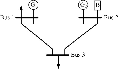
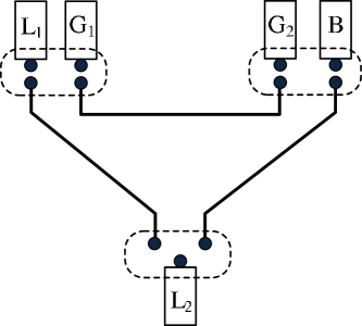
Figure 1: A simple network (left), and its transformation into standard form (right).

The set of terminals can be partitioned by either the devices they are associated with, or the nets in which they are contained. Figure 2 shows the network in figure 1 as a bipartite graph, with devices on the left and nets on the right.

\psfrag{1}{$\mathrm{T}_{3}$}\psfrag{2}{$\mathrm{L}_{2}$}\psfrag{3}{$\mathrm{T}_{2}$}\psfrag{4}{$\mathrm{G}_{2}$}\psfrag{5}{$\mathrm{B}$}\psfrag{6}{$\mathrm{T}_{1}$}\psfrag{7}{$\mathrm{G}_{1}$}\psfrag{8}{$\mathrm{L}_{1}$}\includegraphics[width=130.08731pt]{bipartite_graph.eps}

Figure 2: The network in figure 1 represented as a bipartite graph. Devices (boxes) are shown on the left with their associated terminals (dots). The terminals are connected to their corresponding nets (solid boxes) on the right.

3 Device examples

We present a few examples of how common devices can be modeled in our framework. We note that these examples are intentionally kept simple, but could easily be extended to more refined objectives and constraints. In these examples, it is easier to discuss operational costs and constraints for each device separately. A device’s objective function is equal to the device’s cost function unless any constraint is violated, in which case we set the objective value to $+\infty$.

Generator.

A generator is a single-terminal device with power schedule $p_{\mathrm{gen}}$, which generates power over a range, $P^{\mathrm{min}}\leq-p_{\mathrm{gen}}\leq P^{\mathrm{max}}$, and has ramp-rate constraints

$$R^{\mathrm{min}}\leq-Dp_{\mathrm{gen}}\leq R^{\mathrm{max}},$$

which limit the change of power levels from one period to the next. Here, the operator $D\in{\mbox{\bf R}}^{(T-1)\times T}$ is the forward difference operator, defined as

$$(Dx)(\tau)=x(\tau+1)-x(\tau),\quad\tau=1,\ldots,T-1.$$

The cost function for a generator has the separable form

$$\psi_{\mathrm{gen}}(p_{\mathrm{gen}})=\sum_{\tau=1}^{T}\phi_{\mathrm{gen}}(-p_{\mathrm{gen}}(\tau)),$$

where $\phi:{\mbox{\bf R}}\to{\mbox{\bf R}}$ gives the cost of operating the generator at a given power level over a single time period. This function is typically, but not always, convex and increasing. It could be piecewise linear, or, for example, quadratic:

$$\phi_{\mathrm{gen}}(u)=\alpha u^{2}+\beta u,$$

where $\alpha,\beta>0$.

More sophisticated models of generators allow for them to be switched on or off, with an associated cost each time they are turned on or off. When switched on, the generator operates as described above. When the generator is turned off, it generates no power but can still incur costs for other activities such as idling.

Transmission line.

A transmission line is a two terminal device that transmits power across some distance with power schedules $p_{1}$ and $p_{2}$ and zero cost function. The sum $p_{1}+p_{2}$ represents the loss in the line and is always nonnegative. The difference $p_{1}-p_{2}$ can be interpreted as twice the power flow from terminal one to terminal two. A line has a maximum flow capacity, which is given by

$$|p_{1}-p_{2}|\leq C^{\mathrm{max}},$$

as well as a loss function, $\ell(p_{1},p_{2}):{\mbox{\bf R}}^{2\times T}\to{\mbox{\bf R}}^{T}_{+}$, which defines the constraint

$$p_{1}+p_{2}+\ell(p_{1},p_{2})=0.$$

In many cases, $\ell$ is a convex function with $\ell(0,0)=0$. Under a simple resistive model, $\ell$ is a convex quadratic function of $p_{1}$ and $p_{2}$. Under a model for AC power transmission, the feasible region defined by power loss is given by an ellipse [LTZ12].

Battery.

A battery is a single terminal energy storage device with power schedule $p_{\mathrm{bat}}$, which can take in or deliver energy, depending on whether it is charging or discharging. The charging and discharging rates are limited by the constraints $-D^{\mathrm{max}}\leq p_{\mathrm{bat}}\leq C^{\mathrm{max}}$, where $C^{\mathrm{max}}\in{\mbox{\bf R}}^{T}$ and $D^{\mathrm{max}}\in{\mbox{\bf R}}^{T}$ are the maximum charging and discharging rates. At time $t$, the charge level of the battery is given by local variables

$$q(\tau)=q^{\mathrm{init}}+\sum_{t=1}^{\tau}p_{\mathrm{bat}}(t),\quad\tau=1,\ldots,T,$$

where $q^{\mathrm{init}}$ is the initial charge. It has zero cost function and the charge level must not exceed the battery capacity, i.e., $0\leq q(\tau)\leq Q^{\mathrm{max}}$, $\tau=1,\ldots,T$. It is common to constrain the terminal battery charge $q(T)$ to be some specified value or to match the initial charge $q^{\mathrm{init}}$.

More sophisticated battery models include (possibly state-dependent) charging and discharging inefficiencies as well as charge leakage. In addition, they can include costs which penalize excessive charge-discharge cycling.

Fixed load.

A fixed energy load is a single terminal device with zero cost function which consists of a desired consumption profile, $l\in{\mbox{\bf R}}^{T}$. This consumption profile must be satisfied in each period, i.e., we have the constraint $p_{\mathrm{load}}=l$.

Thermal load.

A thermal load is a single terminal device with power schedule $p_{\mathrm{therm}}$ which consists of a heat store (room, cooled water reservoir, refrigerator), with temperature profile $\theta\in{\mbox{\bf R}}^{T}$, which must be kept within minimum and maximum temperature limits, $\theta^{\mathrm{min}}\in{\mbox{\bf R}}^{T}$ and $\theta^{\mathrm{max}}\in{\mbox{\bf R}}^{T}$. The temperature of the heat store evolves according to

$$\theta(\tau+1)=\theta(\tau)+(\mu/c)(\theta^{\mathrm{amb}}(\tau)-\theta(\tau))-(\eta/c)p_{\mathrm{therm}}(\tau),\quad\tau=1,\ldots,T-1,\qquad\theta(1)=\theta^{\mathrm{init}},$$

where $0\leq p_{\mathrm{therm}}\leq H^{\mathrm{max}}$ is the cooling power consumption profile, $H^{\mathrm{max}}\in{\mbox{\bf R}}^{T}$ is the maximum cooling power, $\mu$ is the ambient conduction coefficient, $\eta$ is the heating/cooling efficiency, $c$ is the heat capacity of the heat store, $\theta^{\mathrm{amb}}\in{\mbox{\bf R}}^{T}$ is the ambient temperature profile, and $\theta^{\mathrm{init}}$ is the initial temperature of the heat store. A thermal load has zero cost function.

More sophisticated models include temperature-dependent cooling and heating efficiencies for heat pumps, more complex dynamics of the system whose temperature is being controlled, and additional additive terms in the thermal dynamics, to represent occupancy or other heat sources.

Deferrable load.

A deferrable load is a single terminal device with zero cost function that must consume a minimum amount of power over a given interval of time, which is characterized by the constraint $\sum_{\tau=A}^{D}p_{\mathrm{load}}(\tau)\geq E$, where $E$ is the minimum total consumption for the time interval $\tau=A,\ldots,D$. The energy consumption in each time period is constrained by $0\leq p_{\mathrm{load}}\leq L^{\mathrm{max}}$. In some cases, the load can only be turned on or off in each time period, i.e., $p_{\mathrm{load}}(\tau)\in\{0,L^{\mathrm{max}}\}$ for $\tau=A,\ldots,D$.

Curtailable load.

A curtailable load is a single terminal device which does not impose hard constraints on its power requirements, but instead penalizes the shortfall between a desired load profile $l\in{\mbox{\bf R}}^{T}$ and delivered power. In the case of a linear penalty, its cost function is given by

$$\alpha(l-p_{\mathrm{load}})_{+},$$

where $(z)_{+}=\max(0,z)$, $p_{\mathrm{load}}\in{\mbox{\bf R}}^{T}$ is the amount of electricity delivered to the device, and $\alpha>0$ is a penalty parameter.

Electric vehicle.

An electric vehicle is a single terminal device with power schedule $p_{\mathrm{ev}}$ which has a desired charging profile $c^{\mathrm{des}}\in{\mbox{\bf R}}^{T}$ and can be charged within a time interval $\tau=A,\ldots,D$. To avoid excessive charge cycling, we assume that the electric vehicle battery cannot be discharged back into the grid (in more sophisticated vehicle-to-grid models, this assumption is relaxed), so we have the constraints $0\leq p_{\mathrm{ev}}\leq C^{\mathrm{max}}$, where $C^{\mathrm{max}}\in{\mbox{\bf R}}^{T}$ is the maximum charging rate. We assume that $c^{\mathrm{des}}(\tau)=0$ for $\tau\notin\{A,\ldots,D\}$, and for $\tau=A,\ldots,D$, the charge level is given by

$$q(\tau)=q^{\mathrm{init}}+\sum_{t=A}^{\tau}p_{\mathrm{ev}}(t),$$

where $q^{\mathrm{init}}$ is the initial charge of the vehicle when it is plugged in at time $\tau=A$.

We can model electric vehicle charging as a deferrable load, where we require a given charge level to be achieved at some time. A more realistic model is as a combination of a deferrable and curtailable load, with cost function

$$\alpha\sum_{\tau=A}^{D}(c^{\mathrm{des}}(\tau)-q(\tau))_{+},$$

where $\alpha>0$ is a penalty parameter. Here $c^{\mathrm{des}}(\tau)$ is the desired charge level at time $\tau$, and $c^{\mathrm{des}}(\tau)-q(\tau))_{+}$ is the shortfall.

External tie with transaction cost.

An external tie is a connection to an external source of power. We represent this as a single terminal device with power schedule $p_{\mathrm{ex}}$. In this case, $p_{\mathrm{ex}}(\tau)_{-}=\max\{-p_{\mathrm{ex}}(\tau),0\}$ is the amount of energy pulled from the source, and $p_{\mathrm{ex}}(\tau)_{+}=\max\{p_{\mathrm{ex}}(\tau),0\}$ is the amount of energy delivered to the source, at time $\tau$. We have the constraint $|p_{\mathrm{ex}}(\tau)|\leq E^{\mathrm{max}}(\tau)$, where $E^{\mathrm{max}}\in{\mbox{\bf R}}^{T}$ is the transaction limit.

We suppose that the prices for buying and selling energy are given by $c\pm\gamma$ respectively, where $c(\tau)$ is the midpoint price, and $\gamma(\tau)>0$ is the difference between the price for buying and selling (i.e., the transaction cost). The cost function is then

$$-(c-\gamma)^{T}(p_{\mathrm{ex}})_{+}+(c+\gamma)^{T}(p_{\mathrm{ex}})_{-}=-c^{T}p_{\mathrm{ex}}+\gamma^{T}|p_{\mathrm{ex}}|,$$

where $|p_{\mathrm{ex}}|$, $(p_{\mathrm{ex}})_{+}$, and $(p_{\mathrm{ex}})_{-}$ are all interpreted elementwise.

4 Convexity

4.1 Devices

We call a device convex if its objective function is a convex function. A network is convex if all of its devices are convex. For convex networks, the OPSP is a convex optimization problem, which means that in principle we can efficiently find a global solution [BV04]. When the network is not convex, even finding a feasible solution for the OPSP can become difficult, and finding and certifying a globally optimal solution to the OPSP is generally intractable. However, special structure in many practical power distribution problems allows us to guarantee optimality in certain cases.

In the examples from §3, the battery, fixed load, thermal load, curtailable load, electric vehicle, and external tie are all convex devices using the constraints and objective functions given. A deferrable load is convex if we drop the constraint that it can only be turned on or off. We discuss the convexity properties of the generator and transmission line in the following section.

4.2 Relaxations

One technique to deal with non-convex networks is to use convex relaxations. We use the notation $g^{\mathrm{env}}$ to denote the convex envelope [Roc70] of the function $g$. There are many equivalent definitions for the convex envelope, for example, $g^{\mathrm{env}}$ = $(g^{*})^{*}$, where $g^{*}$ denotes the convex conjugate of the function $g$. We can equivalently define $g^{\mathrm{env}}$ to be the largest convex lower bound of $g$. If $g$ is a convex, closed, proper (CCP) function, then $g=g^{\mathrm{env}}$.

We define the relaxed optimal power scheduling problem (rOPSP) as

$$\begin{array}[]{ll}\mbox{minimize}&f^{\mathrm{env}}(p)\\ \mbox{subject to}&\bar{p}=0,\end{array}$$ (4)

with variable $p:\mathcal{T}\to{\mbox{\bf R}}^{T}$. This is a convex optimization problem, whose optimal value can in principle be computed efficiently, and whose optimal objective value is a lower bound for the optimal objective value of the OPSP. In some cases, we can guarantee a priori that a solution to the rOPSP will also be a solution to the OPSP based on a property of the network objective such as monotonicity. Even when the relaxed solution does not satisfy all of the constraints in the unrelaxed problem, it can be used as a starting point to help construct good, local solutions to the unrelaxed problem. The suboptimality of these local solutions can then be bounded by the gap between their network objective and the lower bound provided by the solution to the rOPSP. If this gap is small for a given local solution, we can guarantee that it is nearly optimal.

Generator.

\psfrag{000}[ct][ct]{$0$}\psfrag{001}[ct][ct]{$1$}\psfrag{002}[ct][ct]{$2$}\psfrag{003}[ct][ct]{$3$}\psfrag{004}[ct][ct]{$4$}\psfrag{005}[rc][rc]{$0.4$}\psfrag{006}[rc][rc]{$0.6$}\psfrag{007}[rc][rc]{$0.8$}\psfrag{008}[rc][rc]{$1.0$}\psfrag{009}[rc][rc]{$1.2$}\psfrag{010}[rc][rc]{$1.4$}\psfrag{011}[rc][rc]{$1.6$}\psfrag{pmin}[b][l]{$P^{\mathrm{min}}$}\psfrag{pmax}{$P^{\mathrm{max}}$}\psfrag{pc}{$P^{\mathrm{c}}$}\psfrag{pgen}[t][B]{$-p_{\mathrm{gen}}$}\psfrag{fgen}[b][t]{$\phi_{\mathrm{gen}}(p_{\mathrm{gen}})$}\includegraphics[width=173.44534pt]{generator_normal.eps}

\psfrag{000}[ct][ct]{$0$}\psfrag{001}[ct][ct]{$1$}\psfrag{002}[ct][ct]{$2$}\psfrag{003}[ct][ct]{$3$}\psfrag{004}[ct][ct]{$4$}\psfrag{005}[rc][rc]{$0.4$}\psfrag{006}[rc][rc]{$0.6$}\psfrag{007}[rc][rc]{$0.8$}\psfrag{008}[rc][rc]{$1.0$}\psfrag{009}[rc][rc]{$1.2$}\psfrag{010}[rc][rc]{$1.4$}\psfrag{011}[rc][rc]{$1.6$}\psfrag{pmin}[b][l]{$P^{\mathrm{min}}$}\psfrag{pmax}{$P^{\mathrm{max}}$}\psfrag{pc}{$P^{\mathrm{c}}$}\psfrag{pgen}[t][B]{$-p_{\mathrm{gen}}$}\psfrag{fgen}[b][t]{$\phi_{\mathrm{gen}}^{\mathrm{env}}(p_{\mathrm{gen}})$}\includegraphics[width=173.44534pt]{generator_relax.eps}

Figure 3: Left: Cost function for a generator that can be turned off. Right: Its convex relaxation.

When a generator is modeled as in §3 and is always powered on, it is a convex device. However, when given the ability to be powered on and off, the generator is no longer convex. In this case, we can relax the generator objective function so that its cost for power production in each time period, given in figure 3, is a convex function. This allows the generator to produce power in the interval $[0,P^{\mathrm{min}}]$.

Transmission line.

\psfrag{x}{}\psfrag{y}{}\includegraphics[width=173.44534pt]{line_loss_normal.eps}

\psfrag{x}{}\psfrag{y}{}\includegraphics[width=173.44534pt]{line_loss_relax.eps}

Figure 4: Left: Feasible sets of a transmission lines with no loss (black) and AC loss (grey). Right: Their convex relaxations.

In a lossless transmission line, we have $\ell(p_{1},p_{2})=0$, and thus the set of feasible power schedules is the line segment

$$L=\{(p_{1},p_{2})\mid p_{1}=-p_{2},\quad p_{2}\in[-C^{\mathrm{max}}/2,C^{\mathrm{max}}/2]\},$$

as shown in figure 4 in black. When the transmission line has losses, in most cases the loss function $\ell$ is a convex function of the input and output powers, which leads to a feasible region like the grey arc in figure 4. For example, using a lumped $\Pi$ model and under the common assumption that the voltage magnitude is fixed [BV99], a transmission line with series admittance $g-ib$ gives the quadratic loss

$$\ell(p_{1},p_{2})=-(g/4)((p_{1}+p_{2})^{2}/g^{2}+(p_{1}-p_{2})^{2}/b^{2}).$$ (5)

The feasible set of a relaxed transmission line is given by the convex hull of the original transmission line’s constraints. The right side of figure 4 shows examples of this for both lossless and lossy transmission lines. Physically, this relaxation gives lossy transmission lines the ability to discard some additional power beyond what is simply lost to heat. Since electricity is generally a valuable commodity in power networks, the transmission lines will generally not throw away any additional power in the optimal solution to the rOPSP, leading to the power line constraints in the rOPSP being tight and thus also satisfying the unrelaxed power line constraints in the original OPSP. As was shown in [LTZ12], when the network is a tree, this relaxation is always tight. In addition, when all locational marginal prices are positive and no other non-convexities exist in the network, the tightness of the line constraints in the rOPSP can be guaranteed in the case of networks that have separate phase shifters on each loop in the networks whose shift parameter can be freely chosen [SL12].

5 Decentralized method

We begin this section by deriving the prox-average message passing equations assuming that all the device objective functions are convex closed proper (CCP) functions. We then compare the computational and communication requirements of prox-average message passing with a centralized solver for the OPSP. The additional requirements that the functions are closed and proper are technical conditions that are in practice satisfied by any convex function used to model devices. We note that we do not require either finiteness or strict convexity of any device objective function, and that all results apply to networks with arbitrary topology.

Whenever we have a set of variables that maps terminals to time periods, $x:\mathcal{T}\to{\mbox{\bf R}}^{T}$ (which we can also associate with a $|\mathcal{T}|\times T$ matrix), we will use the same index and over-line notation for the variables $x$ as we do for power schedules $p$. For example, $x_{t}\in{\mbox{\bf R}}^{T}$ consists of the time period vector of values of $x$ associated with terminal $t$ and $\bar{x}_{t}=(1/|n|)\sum_{t^{\prime}\in n}x_{t^{\prime}}$, where $t\in n$, with similar notation for indexing $x$ by devices and nets.

5.1 Prox-average message passing

We derive the prox-average message passing equations by reformulating the OPSP using the alternating direction method of multipliers (ADMM) and then simplifying the resulting equations. We refer the reader to [BPC⁺11] for a thorough overview of ADMM.

We first rewrite the OPSP as

$$\begin{array}[]{ll}\mbox{minimize}&\sum_{d\in\mathcal{D}}f_{d}(p_{d})+\sum_{n\in\mathcal{N}}g_{n}(z_{n})\\ \mbox{subject to}&p=z,\end{array}$$ (6)

with variables $p,z:\mathcal{T}\to{\mbox{\bf R}}^{T}$, where $g_{n}(z_{n})$ is the indicator function on the set $\{z_{n}:\bar{z}_{n}=0\}$. We use the notation from [BPC⁺11] and, ignoring a constant, form the augmented Lagrangian

$$L_{\rho}(p,z,u)=\sum_{d\in\mathcal{D}}f_{d}(p_{d})+\sum_{n\in\mathcal{N}}g_{n}(z_{n})+(\rho/2)\|p-z+u\|_{2}^{2},$$ (7)

with the scaled dual variables $u=y/\rho:\mathcal{T}\to{\mbox{\bf R}}^{T}$, which we associate with a $|\mathcal{T}|\times T$ matrix. Because devices and nets are each partitions of the terminals, the last term of (7) can be split across either devices or nets, i.e.,

$$(\rho/2)\|p-z+u\|_{2}^{2}=\sum_{d\in\mathcal{D}}(\rho/2)\|p_{d}-z_{d}+u_{d}\|_{2}^{2}=\sum_{n\in\mathcal{N}}(\rho/2)\|p_{n}-z_{n}+u_{n}\|_{2}^{2}.$$

The resulting ADMM algorithm is then given by the iterations

$$p_{d}^{k+1} := \mathop{\rm argmin}_{p_{d}}\left(f_{d}(p_{d})+(\rho/2)\|p_{d}-z_{d}^{k}+u_{d}^{k}\|^{2}_{2}\right),\quad d\in\mathcal{D},$$

$$z_{n}^{k+1} := \mathop{\rm argmin}_{z_{n}}\left(g(z_{n})+(\rho/2)\|z_{n}-u_{n}^{k}-p_{n}^{k+1}\|^{2}_{2}\right),\quad n\in\mathcal{N},$$

$$u_{n}^{k+1} := u_{n}^{k}+(p_{n}^{k+1}-z_{n}^{k+1}),\quad n\in\mathcal{N},$$

where the first step is carried out in parallel by all devices, and then the second and third steps are carried out in parallel by all nets.

Since $g_{n}(z_{n})$ is simply an indicator function for each net $n$, the second step of the algorithm can be computed analytically and is given by

$$z^{k+1}_{n} := u^{k}_{n}+p^{k+1}_{n}-\bar{u}^{k}_{n}-\bar{p}^{k+1}_{n}.$$

By plugging this quantity into the $u$ update step, the algorithm can be simplified further to yield the prox-average message passing algorithm:

1. Proximal power schedule update.

   $$p_{d}^{k+1}:=\mathbf{prox}_{f_{d},\rho}(p_{d}^{k}-\bar{p}_{d}^{k}-u_{d}^{k}),\quad d\in\mathcal{D}.$$ (8)

2. Scaled price update.

   $$u_{n}^{k+1}:=u_{n}^{k}+\bar{p}_{n}^{k+1},\quad n\in\mathcal{N}.$$ (9)

The proximal function for a function $f$ is given by

$$\mathbf{prox}_{f,\rho}(x)=\mathop{\rm argmin}_{y}\left(f(y)+(\rho/2)\|x-y\|_{2}^{2}\right),$$ (10)

which is guaranteed to exist when $f$ is CCP [Roc70].

We can now see where the name prox-average message passing comes from. In each iteration, every device computes the proximal function of its objective function, with an argument that depends on messages passed to it through its terminals by its neighboring nets in the previous iteration ($\bar{p}_{d}^{k}$ and $u_{d}^{k}$). Then, every devices passes to its terminals the newly computed power schedules, $p_{d}^{k+1}$, which are then passed to the terminals’ associated nets. Every net computes its new average power imbalance, $\bar{p}_{n}^{k+1}$, updates its dual variables, $u_{n}^{k+1}$, and broadcasts these values to its associated terminals’ devices. Since $\bar{p}_{n}^{k}$ is simply $|n|$ copies of the same vector for all $k$, we can see that all terminals connected to the same net have the same value for their dual variables throughout the algorithm, i.e., for all values of $k$, $u_{t}^{k}=u_{t^{\prime}}^{k}$ whenever $t,t^{\prime}\in n$ for any $n\in\mathcal{N}$.

As an example, consider the network represented by figures 1 and 2. The prox-average algorithm performs the power schedule update on the devices (the boxes on the left in figure 2). The devices share the respective power profiles via the terminals, and the nets (the solid boxes on the right) compute the scaled price update. For any network, the prox-average algorithm can be thought of as alternating between devices (on the left) and nets (on the right).

Convergence.

We make a few comments about the convergence of prox-average message passing. Since prox-average message passing is a version of ADMM, all convergence results that apply to ADMM also apply to prox-average message passing. In particular, when all devices have closed, convex, proper (CCP) objective functions and a feasible solution to the OPSP exists, the following hold.

1. Residual convergence. $\bar{p}^{k}\to 0$ as $k\to\infty$,

2. Objective convergence. $\sum_{d\in\mathcal{D}}f_{d}(p_{d}^{k})+\sum_{n\in\mathcal{N}}g_{n}(p_{n}^{k})\to f^{\star}$ as $k\to\infty$,

3. Dual variable convergence. $\rho u^{k}=y^{k}\to y^{\star}$ as $k\to\infty$,

where $f^{\star}$ is the optimal value for the OPSP, and $y^{\star}$ are the optimal dual variables. The proof of these conditions can be found in [BPC⁺11]. As a result of the third condition, the optimal locational marginal prices $\mathcal{L}^{\star}$ can be found for each net $n\in\mathcal{N}$ by setting $\mathcal{L}_{n}^{\star}=y_{n}^{\star}/|n|$.

Stopping criterion.

Following [BPC⁺11], we can define primal and dual residuals, which for prox-average message passing simplify to

$$r^{k}=\bar{p}^{k},\quad s^{k}=\rho((p^{k}-\bar{p}^{k})-(p^{k-1}-\bar{p}^{k-1})).$$

We give a simple interpretation of each residual. The primal residual is simply the net power imbalance across all nets in the network, which is the original measure of primal feasibility in the OPSP. The dual residual is equal to the difference between the current and previous iterations of the difference between power schedules and their average net power. The locational marginal price at each net is determined by the deviation of all associated terminals’ power schedule from the average power on that net. As the change in these deviations approaches zero, the corresponding locational marginal prices converge to their optimal values.

We can define a simple criterion for terminating prox-average message passing when

$$\|r^{k}\|_{2}\leq\epsilon^{\mathrm{pri}},\quad\|s^{k}\|_{2}\leq\epsilon^{\mathrm{dual}},$$

where $\epsilon^{\mathrm{pri}}$ and $\epsilon^{\mathrm{dual}}$ are, respectively, primal and dual tolerances. We can normalize both of these quantities to network size by the relation

$$\epsilon^{\mathrm{pri}}=\epsilon^{\mathrm{dual}}=\epsilon^{\mathrm{abs}}\sqrt{|\mathcal{T}|T},$$

for some absolute tolerance $\epsilon^{\mathrm{abs}}>0$.

Choosing a value of $\rho$.

Numerous examples show that the value of $\rho$ can have a dramatic effect on the rate of convergence of ADMM and prox-average message passing. Many good methods for picking $\rho$ in both offline and online fashions are discussed in [BPC⁺11]. We note that unlike other versions of ADMM, the scaling parameter $\rho$ enters very simply into the prox-average equations and can thus be modified online without incurring any additional computational penalties, such as having to re-factorize a matrix.

We can modify the prox-average message passing algorithm with the addition of a third step

1. Parameter update and price rescaling.

   $$\rho^{k+1} := h(\rho^{k},r^{k},s^{k}),$$

   $$u^{k+1} := \frac{\rho^{k}}{\rho^{k+1}}u^{k+1},$$

for some function $h$. We desire to pick an $h$ such that the primal and dual residuals are of similar size throughout the algorithm, i.e., $\rho^{k}\|r^{k}\|_{2}\approx\|s^{k}\|_{2}$ for all $k$. To accomplish this task, we use a simple proportional-derivative controller to update $\rho$, choosing $h$ to be

$$h(\rho^{k})=\rho^{k}\exp(\lambda v^{k}+\mu(v^{k}-v^{k-1})),$$

where $v^{k}=\rho^{k}\|r^{k}\|_{2}/\|s^{k}\|_{2}-1$ and $\lambda$ and $\mu$ are nonnegative parameters chosen to control the rate of convergence. Typical values of $\lambda$ and $\mu$ are between $10^{-3}$ and $10^{-1}$.

When $\rho$ is updated in such a manner, convergence is sped up in many examples, sometimes dramatically. Although it can be difficult to prove convergence of the resulting algorithm, a standard trick is to assume that $\rho$ is changed only for a large but bounded number of iterations, at which point it is held constant for the remainder of the algorithm, thus guaranteeing convergence.

Non-convex case.

When one or more of the device objective functions is non-convex, we can no longer guarantee that prox-average message passing converges to the optimal value of the OPSP or even that it converges at all (i.e., reaches a fixed point). Prox functions for non-convex devices must be carefully defined as the set of minimizers in (10) is no longer necessarily a singleton. Even when they can be defined, prox functions of non-convex functions are intractable to compute in many cases.

One solution to these issues is to use prox-average message passing to solve the rOPSP. It is easy to show that $f^{\mathrm{env}}(p)=\sum_{d\in\mathcal{D}}f^{\mathrm{env}}_{d}(p_{d})$. As a result, we can run prox-average message passing using the proximal functions of the relaxed device objective functions. Since $f_{d}^{\mathrm{env}}$ is a CCP function for all $d\in\mathcal{D}$, prox-average message passing in this case is guaranteed to converge to the optimal value of the rOPSP and yield the optimal relaxed locational marginal prices.

5.2 Discussion

In order to compute the prox-average messages, devices and nets only require knowledge of who their network neighbors are, the ability to send small vectors of numbers to those neighbors in each iteration, and the ability to store small amounts of state information and efficiently compute prox functions (devices) or averages (nets). As all communication is local and peer-to-peer, prox-average message passing supports the ad hoc formation of power networks, such as micro grids, and is robust to device failure and unexpected network topology changes.

Due to recent advances in convex optimization [WB10, MB12, MWB11], many of the prox function calculations that devices must perform can be very efficiently executed at millisecond or microsecond time-scales on inexpensive, embedded processors. Since all devices and all nets can each perform their computations in parallel, the time to execute a single, network wide prox-average message passing iteration (ignoring communication overhead) is equal to the sum of the maximum computation time over all devices and the maximum computation time of all nets in the network. As a result, the computation time per iteration is small and essentially independent of the size of the network.

In contrast, solving the OPSP in a centralized fashion requires complete knowledge of the network topology, sufficient communication bandwidth to centrally aggregate all devices objective function data, and sufficient centralized computational resources to solve the resulting OPSP. In large, real-world networks, such as the smart grid, all three of these requirements are generally unattainable. Having accurate and timely information on the global connectivity of all devices is infeasible for all but the smallest of dynamic networks. Centrally aggregating all device objective functions would require not only infeasible bandwidth and data storage requirements at the aggregation site, but also the willingness of all devices to expose what could be proprietary function parameters in their objective functions. Finally, a centralized solution to the OPSP requires solving an optimization problem with $\Omega(|\mathcal{T}|T)$ variables, which leads to an identical lower bound on the time scaling for a centralized solver, even if problem structure is exploited. As a result, the centralized solver cannot scale to solve the OPSP on very large networks.

6 Numerical examples

We illustrate the speed and scaling of prox-average message passing with a range of numerical examples. In the first two sections, we describe how we generate network instances for our examples. We then describe our implementation, showing how multithreading can exploit problem parallelism and how our method would scale in a fully peer-to-peer implementation. Lastly, we present our results, and demonstrate how the number of prox-average iterations needed for convergence is essentially independent of network size and also significantly decreases when the algorithm is seeded with a reasonable warm-start.

6.1 Network topology

We generate a network instance by first picking the number of nets $N$. We generate the locations $x_{i}\in{\mbox{\bf R}}^{2}$, $i=1,\ldots,N$ by drawing them uniformly at random from $[0,\sqrt{N}]^{2}$. (These locations will be used to determine network topology.) Next, we introduce transmission lines into the network as follows. We first connect a transmission line between all pairs of nets $i$ and $j$ independently and with probability

$$\gamma(i,j)=\alpha\min(1,d^{2}/\|x_{i}-x_{j}\|_{2}^{2}).$$

In this way, when the distance between $i$ and $j$ is smaller than $d$, they are connected with a fixed probability $\alpha>0$, and when they are located farther than distance $d$ apart, the probability decays as $1/\|x_{i}-x_{j}\|_{2}^{2}$. After this process, we add a transmission line between any isolated net and its nearest neighbor. We then introduce transmission lines between distinct connected components by selecting two connected components uniformly at random and then selecting two nets, one inside each component, uniformly at random and connecting them by a transmission line. We continue this process until the network is connected.

For the network instances we present, we chose parameter values $d=0.15$ and $\alpha=0.8$ as the parameters for generating our network. This results in networks with an average degree of $2.3$. Using these parameters, we generated networks with $100$ to $100000$ nets, which resulted in optimization problems with approximately $30$ thousand to $30$ million variables.

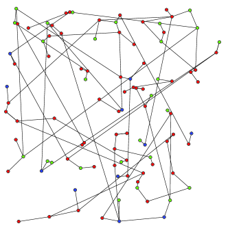
Figure 5: A sample random network. Devices are color-coded: generators are in green, batteries are in blue, and loads are in red. Edges represent transmission lines.

6.2 Devices

After we generate the network topology described above, we randomly attach a single (one-terminal) device to each net according to the distribution in table 1. The models for each device in the network are identical to the ones given in section 3, with model parameters chosen in a manner we describe below. Figure 5 shows an example network for $N=100$ ($30$ thousand variables) generated in this fashion.

For simplicity, our examples only include networks with the devices listed below. For all devices, the time horizon was chosen to be $T=96$, indicating $15$ minute intervals for a $24$ hour power schedule, with the time period $\tau=1$ corresponding to midnight.

Device	Fraction
Generator	$0.2$
Battery	$0.1$
Fixed load	$0.5$
Deferrable load	$0.1$
Curtailable load	$0.1$

Table 1: Fraction of one-terminal devices present in the generated networks.

Generator.

Generators have the quadratic cost functions given in §3 and are divided into three types: small, medium, and large. In each case, we allow the generator to be turned on and off by setting $P_{\mathrm{min}}=0$. Small generators have the smallest maximum power output, but the largest ramp rates, while large generators have the largest maximum power output, but the slowest ramp rates. Medium generators lie in between. Large generators are generally more efficient than small and medium generators which is reflected in their cost function by having smaller values of $\alpha$ and $\beta$. Whenever a generator is placed into a network, its type is selected uniformly at random, and its parameters are taken from the appropriate row in table 2.

	$P^{\mathrm{min}}$	$P^{\mathrm{max}}$	$R^{\mathrm{max}}$	$\alpha$	$\beta$
Large	$0$	$50$	$3$	$0.001$	$0.1$
Medium	$0$	$20$	$5$	$0.005$	$0.2$
Small	$0$	$10$	$10$	$0.02$	$1$

Table 2: Generator parameters.

Battery.

For a given instance of a battery, its parameters are generated by setting $q^{\mathrm{init}}=0$ and selecting $Q^{\mathrm{max}}$ uniformly at random from the interval $[20,50]$. The charging and discharging rates are selected to be equal (i.e., $C^{\mathrm{max}}=D^{\mathrm{max}}$) and drawn uniformly at random from the interval $[5,10]$.

Fixed load.

The load profile for a fixed load instance is a sinusoid,

$$l(\tau)=c+a\sin(2\pi(\tau-\phi_{0})/T),\quad\tau=1,\ldots,T,$$

with the amplitude $a$ chosen uniformly at random from the interval $[1,5]$, and the DC term $c$ chosen so that $c=a+u$, where $u$ is chosen uniformly at random from the interval $[0,0.5]$, which ensures that the load profile remains elementwise positive. The phase shift $\phi_{0}$ is chosen uniformly at random from the interval $[60,72]$, ensuring that the load profile peaks between the hours of $3$pm and $6$pm.

Deferrable load.

For an instance of a deferrable load, we choose $E$ uniformly at random from the interval $[500,1000]$. The start time index $A$ is chosen uniformly at random from the discrete set $\{1,\ldots,T-7\}$. The end time index $D$ is then chosen uniformly at random over the set $\{A+7,\ldots,T\}$, so that the minimum time window to satisfy the load is $8$ time periods ($2$ hours). We set the maximum power so that it is possible to satisfy the total energy constraint by only operating in half of the available time periods, i.e., $L^{\mathrm{max}}=2E/(D-A)$.

Curtailable loads.

For an instance of a curtailable load, the desired load $l$ is constant over all time periods with a magnitude chosen uniformly at random from the interval $[5,15]$. The penalty parameter $\alpha$ is chosen uniformly at random from the interval $[1,2]$.

Transmission line.

For an instance of a transmission line, we choose its parameters by first solving the OPSP with lossless, uncapacitated lines, where we add a small quadratic cost function $\epsilon(p_{1}^{2}+p_{2}^{2})$, with $\epsilon=10^{-3}$, to each transmission line in order to help spread power flow throughout the network. Using the flow values given by the solution to that problem, we set $C^{\mathrm{max}}=\max(10,4F^{\mathrm{max}})$ for each line, where $F^{\mathrm{max}}$ is equal to the maximum flow (from the solution to the lossless problem) along that line over all time periods. We use the loss function for transmission lines with a series admittance $g-ib$ given by (5). We choose $g$ and $b$ such that $b=\gamma g$, where $\gamma$ is chosen uniformly at random from the interval $[4.5,5.5]$; on average, the susceptance is $5$ times larger than the conductance. After we pick $C^{\mathrm{max}}$ and $\gamma$, the values of $g$ and $b$ are chosen such that the loss when transmitting power at maximum capacity is uniformly at random between $5$ to $15$ percent of $C^{\mathrm{max}}$.

6.3 Serial multithreaded implementation

Our OPSP solver is implemented in C++, with the core prox-average message passing equations occupying fewer than $25$ lines of C++ (excluding problem setup and classes). The code is compiled with gcc $4.4.5$ on an $8$-core, $3.4$GHz Intel Xeon processor with $16$GB of RAM running the Debian OS. We used the compiler option -O3 to leverage full code optimization.

To approximate a fully distributed implementation, we use gcc’s implementation of OpenMP (version $3.0$) and multithreading to parallelize the computation of the prox functions for the devices. We use $8$ threads (one per core) to solve each example. Assuming perfect load balancing, this means that $8$ prox functions are being evaluated in parallel. Effectively, we evaluate the prox functions by stepping serially through the devices in blocks of size $8$. We do not, however, parallelize the computation of the dual update over the nets since the overhead of spawning threads dominates the vector operation itself.

The prox functions for fixed loads and curtailable loads are separable over $\tau$ and can be computed analytically. For more complex devices, such as a generator, battery, or deferrable load, we compute the prox function using CVXGEN [MB12]. The prox function for a transmission line is computed by projecting onto the convex hull of the line constraints.

For a given network, we solve the associated OPSP with an absolute tolerance $\epsilon^{\mathrm{abs}}=10^{-3}$. This translates to three digits of accuracy in the solution. The CVXGEN solvers used to evaluate the prox operators for some devices have an absolute tolerance of $10^{-8}$. For our $\rho$-update function, $h$, we use the parameter values $\lambda=0.005$ and $\mu=0.01$ and clip our values of $\rho$ to be between $\epsilon^{\mathrm{abs}}$ and $1/\epsilon^{\mathrm{abs}}$ to prevent roundoff error.

6.4 Peer-to-peer implementation

We have not yet created a fully peer-to-peer, bulk synchronous parallel [Val90, MAB⁺10] implementation of prox-average message passing, but have carefully tracked prox-average solve times in our serial implementation in order to facilitate a first order analysis of such a system. In a peer-to-peer implementation, the proximal power schedule updates occur in parallel across all devices followed by (scaled) price updates occurring in parallel across all nets. As previously mentioned, the computation time per prox-average iteration is thus the maximum time, over all devices, to evaluate the proximal function of their objective, added to the maximum time across all nets to average their terminal power schedules and add that quantity to their existing price vector. Since evaluating the prox function for some devices requires solving a convex optimization problem, whereas the price update only requires a small number of vector operations that can be performed as a handful of SIMD instructions, the compute time for the price update is negligible in comparison to the proximal power schedule update. The determining factor in solve time, then, is in evaluating the prox functions for the power schedule update. In our examples, the maximum time taken to evaluate any prox function is $1$ ms. To solve a problem with $N=100000$ nets ($30$ million variables) with approximately $500$ iterations of our prox-average algorithm then takes only $500$ ms.

In practice, the actual solve time would clearly be dominated by network communication latencies and actual runtime performance will be determined by how quickly and reliably packets can be delivered. As a result, in a true peer-to-peer implementation, a negligible amount of time is actually spent on computation. However, it goes without saying that many other issues must be addressed with a peer-to-peer protocol, including handling network delays and security.

6.5 Results

We first consider a single example: a network instance with $N=3000$ ($1$ million variables). Figure 6 shows that after fewer than $500$ iterations of prox-average message passing, both the relative suboptimality and the average net power imbalance are both less than $10^{-3}$. The convergence rates for other network instances over the range of sizes we simulated are similar.

\psfrag{iter}[t][b]{\makebox(0.0,20.0)[1]{\small iter $k$}}\psfrag{obj}[b][t]{\makebox(0.0,50.0)[1]{\small$|f^{k}-f^{\star}|/f^{\star}$}}\psfrag{1}[r][r]{\small$10^{-7}$}\psfrag{2}[r][r]{\small$10^{-5}$}\psfrag{3}[r][r]{\small$10^{-3}$}\psfrag{4}[r][r]{\small$10^{-2}$}\psfrag{5}[r][r]{\small$10^{1}$}\psfrag{0}[t][b]{\small$0$}\psfrag{250}[t][b]{\small$250$}\psfrag{500}[t][b]{\small$500$}\psfrag{750}[t][b]{\small$750$}\psfrag{1000}[t][b]{\small$1000$}\includegraphics[width=173.44534pt]{objective}

\psfrag{iter}[t][b]{\makebox(0.0,20.0)[1]{\small iter $k$}}\psfrag{pbar}[b][t]{\makebox(0.0,50.0)[1]{\small$\|\overline{p}^{k}\|_{2}/\sqrt{|\mathcal{T}|T}$}}\psfrag{1}[r][r]{\small$10^{-7}$}\psfrag{2}[r][r]{\small$10^{-5}$}\psfrag{3}[r][r]{\small$10^{-3}$}\psfrag{4}[r][r]{\small$10^{-2}$}\psfrag{5}[r][r]{\small$10^{1}$}\psfrag{0}[t][b]{\small$0$}\psfrag{250}[t][b]{\small$250$}\psfrag{500}[t][b]{\small$500$}\psfrag{750}[t][b]{\small$750$}\psfrag{1000}[t][b]{\small$1000$}\includegraphics[width=173.44534pt]{primal}

Figure 6: The relative suboptimality (left) and primal infeasibility (right) of prox-average message passing on a network instance with $N=3000$ nets ($1$ million variables). The dashed line shows when the stopping criterion is satisfied.

In figure 7, we present average timing results for solving the OPSP for a family of examples, with networks of size $N=100$, $300$, $1000$, $3000$, $10000$, $30000$, and $100000$. For each network size, we generated and solved $20$ network instances to generate average solve times and confidence intervals around those averages. For network instances with $N=100000$ nets, the problem has approximately $30$ million variables, which we solve serially using prox-average message passing in $52$ minutes on average.

For a peer-to-peer implementation, the runtime of prox-average message passing should be essentially constant, and in particular independent of the size of the network. For our multithreaded implementation, with bounded computation, this would be reflected by a runtime that only increases linearly with the number of nets in a network instance. By fitting a line to figure 7, we find that our parallel implementation scales as $O(N^{0.923})$. The slight discrepancy between this and the ideal exponent of $1$ is accounted for by implementation details such as operating system background processes consuming some compute cycles and slightly imperfect load balancing across all $8$ cores in our system, especially for smaller values of $N$.

\psfrag{N}[t][b]{$N$}\psfrag{time}[b][t]{time (seconds)}\psfrag{1}[r][r]{\small$1$}\psfrag{10}[r][r]{\small$10$}\psfrag{100}[r][r]{\small$100$}\psfrag{1000}[r][r]{\small$1000$}\psfrag{10000}[r][r]{\small$10000$}\psfrag{20}[t]{\small$100$}\psfrag{200}[t]{\small$1000$}\psfrag{2000}[t]{\small$10000$}\psfrag{20000}[t]{\small$100000$}\includegraphics[width=260.17464pt]{runtime}

Figure 7: Average prox-average execution times for a family of networks on $8$ cores. Error bars show $95\%$ confidence bounds. The dotted line shows the least-squares fit to the data on a log-log scale, resulting in an exponent of $0.923$.

We note that figure 7 shows cold start runtimes for solving the OPSP. If we have access to a good estimate of the power schedules and locational marginal prices for each terminal, we can use these estimates to warm start our OPSP solver. To show the effect of warm-starting, we solve a specific problem instance with $N=3000$ nets ($1$ million variables). We define $K^{\mathrm{cold}}$ to be the number of iterations needed to solve an instance of this problem. We then uniformly scale the load profiles of each device by separate and independent lognormal random variables. The new load profiles, $\hat{l}$, are obtained from the original load profiles $l$ according to

$$\hat{l}=l\exp(\sigma X),$$

where $X\sim\mathcal{N}(0,1)$, and $\sigma>0$ is given. Using the solution of the original problem to warm start our solver, we solve the perturbed problem and report the number of iterations $K^{\mathrm{warm}}$ needed to solve it. Figure 8 shows the ratio $K^{\mathrm{warm}}/K^{\mathrm{cold}}$ as we vary $\sigma$, and indicates the significant computational savings that warm-starting can achieve, even under relatively large perturbations.

\psfrag{iters}[b][t]{\makebox(0.0,40.0)[1]{\small$K^{\mathrm{warm}}/K^{\mathrm{cold}}$}}\psfrag{sigma}[t][b]{\makebox(0.0,20.0)[1]{\small$\sigma$}}\psfrag{0}[r]{\small$0$}\psfrag{0.2}[r]{\small$0.2$}\psfrag{0.4}[r]{\small$0.4$}\psfrag{0.6}[r]{\small$0.6$}\psfrag{0.8}[r]{\small$0.8$}\psfrag{1}[r]{\small$1.0$}\psfrag{10}[t]{\small$0.00$}\psfrag{20}[t]{\small$0.05$}\psfrag{30}[t]{\small$0.10$}\psfrag{40}[t]{\small$0.15$}\psfrag{50}[t]{\small$0.20$}\includegraphics[width=173.44534pt]{warmstart}

Figure 8: Number of warm start iterations needed to converge for various perturbations of load profiles.

7 Extensions

Receding horizon control.

The speed with which prox-average message passing converges on very large networks shows its applicability in coordinating real time decisions across massive networks of devices. A direct extension of our work to real-time network operation can be achieved using receding horizon control (RHC) [Mac02, Bem06]. In RHC, we solve the OPSP at each time step to determine conditional consumption and generation profiles for every device over the next $T$ time periods. We then execute the first step of these profiles and resolve the OPSP using new information and measurements that have become available. RHC has been successfully applied to a wide range of areas, including power systems, and allows us to take advantage of warm starting our algorithm, which we have shown to significantly decrease the number of iterations needed for convergence.

Hierarchical models.

The power gird has a natural hierarchy, with generation and transmission occurring at the highest level and residential consumption and distribution occurring at the most granular. Prox-average message passing can be easily extended into hierarchical interactions by scheduling messages on different time scales and between systems at the similar levels of the hierarchy [CLCD07].

We can recursively apply prox-average message passing at each level of the hierarchy. At the highest level, all regional systems exchange their proximal updates once they have computed their own prox-function. It can be shown that computing this function for a given region is equivalent to computing a partial minimization over the sum of the objective functions of devices located inside that region, subject to intra-region power balance. This too can be computed using prox-average message passing. This process can be continued down to the individual device level, at which point the device must solve its own prox function directly as the base case.

Local stopping criteria and $\rho$ updates.

The stopping criterion and the algorithm we propose to update $\rho$ in §5 both currently require global device coordination — specifically the global values of the primal and dual residuals at each iteration. In principle, these could be computed in a decentralized fashion across the network by gossip algorithms [Sha08], but that would require many rounds of gossip in between each iteration of prox-average message passing, significantly increasing runtime. We are currently investigating methods by which both the stopping criterion and different values of $\rho$ can be independently chosen by individual devices or even individual terminals, all based only on local information, such as the primal and dual residuals of a given device and its neighboring nets.

8 Conclusion

We have presented a fully decentralized method for dynamic network energy management based on message passing between devices. Prox-average message passing is simple and highly extensible, relying solely on peer to peer communication between devices that exchange energy. When the resulting network optimization problem is convex, prox-average message passing converges to the optimal value and gives optimal locational marginal prices. We have presented a parallel implementation that shows the time per iteration and the number of iterations needed for convergence of prox-average message passing are essentially independent of the size of the network. As a result, prox-average message passing can scale to extremely large networks with almost no increase in solve time.

References

- [Bal06] R. Baldick. Applied Optimization: Formulation and Algorithms for Engineering Systems. Cambridge University Press, 2006.
- [Bem06] A. Bemporad. Model predictive control design: New trends and tools. In Proceedings of 45th IEEE Conference on Decision and Control, pages 6678–6683, 2006.
- [Ber82] D. P. Bertsekas. Constrained Optimization and Lagrange Multiplier Methods. Academic Press, 1982.
- [BPC+11] S. Boyd, N. Parikh, E. Chu, B. Peleato, and J. Eckstein. Distributed optimization and statistical learning via the alternating direction method of multipliers. Foundations and Trends in Machine Learning, 3:1–122, 2011.
- [BV99] A. Bergen and V. Vittal. Power Systems Analysis. Prentice Hall, 1999.
- [BV04] S. Boyd and L. Vandenberghe. Convex Optimization. Cambridge University Press, 2004. Available at http://www.stanford.edu/~boyd/cvxbook/bv_cvxbook.pdf.
- [Car62] J. Carpentier. Contribution to the economic dispatch problem. Bull. Soc. Francaise Elect., 3(8):431–447, 1962.
- [CI12] E. A. Chakrabortty and M. D. Ilic. Control & Optimization Methods for Electric Smart Grids. Springer, 2012.
- [CLCD07] M. Chiang, S. Low, A. Calderbank, and J. Doyle. Layering as optimization decomposition: A mathematical theory of network architectures. Proc. of the IEEE, 95(1):255–312, 2007.
- [CR90] B. H. Chowdhury and S. Rahman. A review of recent advances in economic dispatch. IEEE Transactions on Power Systems, 5(4):1248–1259, 1990.
- [DW60] G. B. Dantzig and P. Wolfe. Decomposition principle for linear programs. Operations Research, 8:101–111, 1960.
- [Eck94] J. Eckstein. Parallel alternating direction multiplier decomposition of convex programs. Journal of Optimization Theory and Applications, 80(1):39–62, 1994.
- [ET11] J. H. Eto and R. J. Thomas. Computational needs for the next generation electric grid. In Department of Energy, 2011. http://certs.lbl.gov/pdf/lbnl-5105e.pdf.
- [Eve63] H. Everett. Generalized Lagrange multiplier method for solving problems of optimum allocation of resources. Operations Research, 11(3):399–417, 1963.
- [EW02] A. Eydeland and K. Wolyniec. Energy and Power Risk Management: New Developments in Modeling, Pricing and Hedging. Wiley, 2002.
- [GM75] R. Glowinski and A. Marrocco. Sur l’approximation, par elements finis d’ordre un, et la resolution, par penalisation-dualité, d’une classe de problems de Dirichlet non lineares. Revue Française d’Automatique, Informatique, et Recherche Opérationelle, 9:41–76, 1975.
- [GM76] D. Gabay and B. Mercier. A dual algorithm for the solution of nonlinear variational problems via finite element approximations. Computers and Mathematics with Applications, 2:17–40, 1976.
- [Hap77] H. H. Happ. Optimal power dispatch - a comprehensive survey. IEEE Transactions on Power Apparatus and Systems, 96(3):841–854, 1977.
- [Hes69] M. R. Hestenes. Multiplier and gradient methods. Journal of Optimization Theory and Applications, 4:302–320, 1969.
- [KB97] B. H. Kim and R. Baldick. Coarse-grained distributed optimal power flow. IEEE Transactions on Power Systems, 12(2):932–939, 1997.
- [KB00] B. H. Kim and R. Baldick. A comparison of distributed optimal power flow algorithms. IEEE Transactions on Power Systems, 15(2):599–604, 2000.
- [LL12] J. Lavaei and S. Low. Zero duality gap in optimal power flow problem. IEEE Transactions on Power Systems, 27(1):92–107, 2012.
- [LTZ12] J. Lavaei, D. Tse, and B. Zhang. Geometry of power flows in tree networks. To appear, IEEE Power & Energy Society General Meeting, 2012.
- [LVH12] J. Liang, G. K. Venayagamoorthy, and R. G. Harley. Wide-area measurement based dynamic stochastic optimal power flow control for smart grids with high variability and uncertainty. IEEE Transactions on Smart Grid, 3:59–69, 2012.
- [LZT11] A. Lam, B. Zhang, and D. Tse. Distributed algorithms for optimal power flow problem. http://arxiv.org/abs/1109.5229, 2011.
- [MAB+10] G. Malewicz, M. H. Austern, A. J. C. Bik, J. C. Dehnert, I. Horn, N. Leiser, and G. Czajkowski. Pregel: A system for large-scale graph processing. In Proceedings of the 2010 International Conference on Management of Data, pages 135–146, 2010.
- [Mac02] J. Maciejowski. Predictive Control with Constraints. Prentice Hall, 2002.
- [MB12] J. Mattingley and S. Boyd. CVXGEN: Automatic convex optimization code generation. http://cvxgen.com/, 2012.
- [MWB11] J. Mattingley, Y. Wang, and S. Boyd. Receding horizon control: Automatic generation of high-speed solvers. IEEE Control Systems Magazine, 31:52–65, 2011.
- [Pow69] M. J. D. Powell. A method for nonlinear constraints in minimization problems. In R. Fletcher, editor, Optimization. Academic Press, 1969.
- [RAW10] P. Ravikumar, A. Agarwal, and M. J. Wainwright. Message-passing for graph-structured linear programs: Proximal methods and rounding schemes. Journal of Machine Learning Research, 11:1043–1080, 2010.
- [Roc70] R. T. Rockafellar. Convex Analysis. Princeton University Press, 1970.
- [Sha08] D. Shah. Gossip algorithms. Foundations and Trends in Networking, 3(2):1–125, 2008.
- [SL12] S. Sojoudi and J. Lavaei. Physics of power networks makes hard problems easy to solve. To appear, IEEE Power & Energy Society General Meeting, 2012.
- [TSBC11] K. Turitsyn, P. Sulc, S. Backhaus, and M. Chertkov. Options for control of reactive power by distributed photovoltaic generators. Proceedings of the IEEE, 99:1063–1073, 2011.
- [Val90] L. G. Valiant. A bridging model for parallel computation. Communications of the ACM, 33(8):111, 1990.
- [WB10] Y. Wang and S. Boyd. Fast model predictive control using online optimization. IEEE Transactions on Control Systems Technology, 18:267–278, 2010.
- [Zhu09] J. Zhu. Optimization of Power System Operation. Wiley-IEEE Press, 2009.