Knot Universes in Bianchi Type I Cosmology

Abstract

We investigate the trefoil and figure-eight knot universes from Bianchi-type I cosmology. In particular, we construct several concrete models describing the knot universes related to the cyclic universe and examine those cosmological features and properties in detail. Finally some examples of unknotted closed curves solutions (spiky and Mobius strip universes) are presented.

1 Introduction

Inflation is one of the most important phenomena in modern cosmology and has been confirmed by recent observations on cosmic microwave background (CMB) radiation [1]. Furthermore, it is suggested by the cosmological and astronomical observations of Type Ia Supernovae [2], CMB radiation [1], large scale structure (LSS) [3], baryon acoustic oscillations (BAO) [4], and weak lensing [5] that the expansion of the current universe is accelerating. In order to explain the late time cosmic acceleration, we need to introduce so-called dark energy in the framework of general relativity or modify the gravitational theory, which can be regarded as a kind of geometrical dark energy (for reviews on dark energy, see, e.g., [6]-[11], and for reviews on modified gravity, see, e.g., [12]-[17]).

It is considered that there happened a Big Bang singularity in the early universe. In addition, at the dark energy dominated stage, the finite-time future singularities will occur [18]-[23]. There also exists the possibility that a Big Crunch singularity will happen. To avoid such cosmological singularities, there are various proposals such as the cyclic universe [24]-[26] (in other approach of the cyclic universe, see [27]), the ekpyrotic scenario [28], and the bouncing universe [29].

On the other hand, as a related theory to the cyclic universe, the trefoil and figure-eight knot universes have been explored in Ref. [30]. In the homogeneous and isotropic Friedmann-Lemaître-Robertson-Walker (FLRW) and the homogeneous and anisotropic Bianchi-type I cosmologies, the geometrical description of these knot theories corresponds to oscillating solutions of the gravitational field equations. Note that the terms ”the trefoil knot universe” and ”the figure-eight knot universe” were introduced for the first time in Ref. [30]. Moreover, the Weierstrass $\wp(t)$, $\zeta(t)$ and $\sigma(t)$ functions and the Jacobian elliptic functions have been applied to solve several issues on astrophysics and cosmology [31]. In particular, very recently, by combining the reconstruction method in Refs. [12, 22, 33, 34] with the Weierstrass and Jacobian elliptic functions, the equation of state (EoS) for the cyclic universes [35] and periodic generalizations of Chaplygin gas type models [36]-[38] for dark energy [39] have been examined. This procedure can be considered to a novel approach to cosmological models in order to investigate the properties of dark energy.

In this paper, we explore the cosmological features and properties of the trefoil and figure-eight knot universes from Bianchi-type I cosmology in detail. In particular, we construct several concrete models describing the trefoil and figure-eight knot universes based on Bianchi-type I spacetime. In our previous work [30], the models of the knot universes from the homogeneous and isotropic FLRW spacetime were studied. By using the equivalent procedure, as continuous investigations, in this work we explicitly demonstrate that the knot universes can be constructed by Bianchi-type I spacetime. In other words, our purpose is to establish the formalism which can describe the knot universes.

It is significant to emphasize that according to the recent cosmological data analysis [1], it is implied that the universe is homogeneous and isotropic. In fact, however, recently the feature of anisotropy of cosmological phenomena such as anisotropic inflation [46] has also been studied in the literature. In such a cosmological sense, it can be regarded as reasonable to consider the anisotropic universe including Bianchi-type I spacetime. The units of the gravitational constant $8\pi G=c=1$ with $G$ and $c$ being the gravitational constant and the seed of light are used.

The organization of the paper is as follows. In Sec. II, we explain the model and derive the basic equations. In Sec. III, we investigate the trefoil knot universe. Next, we study the figure-eight knot universe in Sec. IV. In Sec. V we present some unknotted closed curve solutions of the model. Finally, we give conclusions in Sec. VI.

2 The model

In this section we briefly review some basic facts about the Einstein’s field equation. We start from the standard gravitational action (chosen units are $c=8\pi G=1$)

$$S=\frac{1}{4}\int d^{4}x\sqrt{-g}(R-2\Lambda+L_{m}),$$ (2.1)

where $R$ is the Ricci scalar, $\Lambda$ is the cosmological constant and $L_{m}$ is the matter Lagrangian. For a general metric $g_{\mu\nu}$, the line element is

$$ds^{2}=g_{\mu\nu}dx^{\mu}dx^{\nu},\ \ (\mu,\nu=0,1,2,3).$$ (2.2)

The corresponding Einstein field equations are given by

$$R_{\mu\nu}+\Big{(}\Lambda-\frac{1}{2}R\Big{)}g_{\mu\nu}=-\kappa^{2}T_{\mu\nu},$$ (2.3)

where $R_{\mu\nu}$ is the Ricci tensor. This equation forms the mathematical basis of the theory of general relativity. In (2.3), $T_{\mu\nu}$ is the energy-momentum tensor of the matter field defined as

$$T_{\mu\nu}=\frac{2}{\sqrt{-g}}\frac{\delta L_{m}}{\delta g^{\mu\nu}},$$ (2.4)

and satisfies the conservation equation

$$\nabla_{\mu}T^{\mu\nu}=0,$$ (2.5)

where $\nabla_{\mu}$ is the covariant derivative which is the relevant operator to smooth a tensor on a differentiable manifold. Eq.(2.5) yields the conservations of energy and momentums, corresponding to the independent variables involved. The general Einstein equation (2.3) is a set of non-linear partial differential equations. We consider the Bianchi - I metric

$$ds^{2}=-d\tau^{2}+A^{2}dx_{1}^{2}+B^{2}dx_{2}^{2}+C^{2}dx_{3}^{2},$$ (2.6)

where we assume that $\tau=t/t_{0},x_{i}=x_{i}^{\prime}/x_{i0},A,B,C$ are dimensionless (usually we put $t_{0}=x_{i0}=1$). Here the metric potentials $A,B$ and $C$ are functions of $\tau=t$ alone. This insures that the model is spatially homogeneous. The statistical volume for the anisotropic Bianchi type-I model can be written as

$$V=ABC.$$ (2.7)

The Ricci scalar is

$$R=g^{ij}R_{ij}=2\left(\frac{\ddot{A}}{A}+\frac{\ddot{B}}{B}+\frac{\ddot{C}}{C}+\frac{\dot{A}\dot{B}}{AB}+\frac{\dot{A}\dot{C}}{AC}+\frac{\dot{B}\dot{C}}{BC}\right),$$ (2.8)

where $\dot{A}=dA/d\tau$ and so on. The non-vanishing components of Einstein tensor

$$G_{ij}=R_{ij}-0.5g_{ij}R$$ (2.9)

are

$$G_{00} = \frac{\dot{A}\dot{B}}{AB}+\frac{\dot{A}\dot{C}}{AC}+\frac{\dot{B}\dot{C}}{BC},$$ (2.10)

$$G_{AA} = -A^{2}\left(\frac{\ddot{B}}{B}+\frac{\ddot{C}}{C}+\frac{\dot{B}\dot{C}}{BC}\right),$$ (2.11)

$$G_{BB} = -B^{2}\left(\frac{\ddot{A}}{A}+\frac{\ddot{C}}{C}+\frac{\dot{A}\dot{C}}{AC}\right),$$ (2.12)

$$G_{CC} = -C^{2}\left(\frac{\ddot{B}}{B}+\frac{\ddot{A}}{A}+\frac{\dot{B}\dot{A}}{BA}\right).$$ (2.13)

We define $a=(ABC)^{\frac{1}{3}}$ as the average scale factor so that the average Hubble parameter may be defined as

$$H=\frac{\dot{a}}{a}=\frac{1}{3}\left(\frac{\dot{A}}{A}+\frac{\dot{B}}{B}+\frac{\dot{C}}{C}\right).$$ (2.14)

We write this average Hubble parameter $H$ sometimes as

$$H=\frac{1}{3}\left(H_{1}+H_{2}+H_{3}\right),$$ (2.15)

where

$$H_{1}=\frac{\dot{A}}{A},\quad H_{2}=\frac{\dot{B}}{B},\quad H_{3}=\frac{\dot{C}}{C}$$ (2.16)

are the directional Hubble parameters in the directions of $x_{1},x_{2}$ and $x_{3}$ respectively. Hence we get the important relations

$$A=A_{0}e^{\int H_{1}dt},\quad B=B_{0}e^{\int H_{2}dt},\quad C=C_{0}e^{\int H_{3}dt},$$ (2.17)

where $A_{0},B_{0},C_{0}$ are integration constants. The other important cosmological quantity is the deceleration parameter $q$, which for our model reads as

$$q=-\frac{a\ddot{a}}{\dot{a}^{2}}.$$ (2.18)

Next, we assume that the energy-momentum tensor of fluid has the form

$$T_{ij}=diag[T_{00},T_{11},T_{22},T_{33}]=diag[\rho,-p_{1},-p_{2},-p_{3}].$$ (2.19)

Here $p_{i}$ are the pressures along the $x_{i}$ axes recpectively, $\rho$ is the proper density of energy. Then the Einstein equations (with gravitational units, $8\pi G=1$ and $c=1$) read as

$$R_{ij}-\frac{1}{2}Rg_{ij}=-T_{ij},$$ (2.20)

where we assumed $\Lambda=0$. For the metric (2.6) these equations take the form

$$\frac{\dot{A}\dot{B}}{AB}+\frac{\dot{B}\dot{C}}{BC}+\frac{\dot{C}\dot{A}}{CA}-\rho = 0,$$ (2.21)

$$\frac{\ddot{B}}{B}+\frac{\ddot{C}}{C}+\frac{\dot{B}\dot{C}}{BC}+p_{1} = 0,$$ (2.22)

$$\frac{\ddot{C}}{C}+\frac{\ddot{A}}{A}+\frac{\dot{C}\dot{A}}{CA}+p_{2} = 0,$$ (2.23)

$$\frac{\ddot{A}}{A}+\frac{\ddot{B}}{B}+\frac{\dot{A}\dot{B}}{AB}+p_{3} = 0.$$ (2.24)

In terms of the Hubble parameters this system takes the form

$$H_{1}H_{2}+H_{2}H_{3}+H_{1}H_{3}-\rho = 0,$$ (2.25)

$$\dot{H}_{2}+\dot{H}_{3}+H^{2}_{2}+H^{2}_{3}+H_{2}H_{3}+p_{1} = 0,$$ (2.26)

$$\dot{H}_{3}+\dot{H}_{1}+H^{2}_{3}+H^{2}_{1}+H_{3}H_{1}+p_{2} = 0,$$ (2.27)

$$\dot{H}_{1}+\dot{H}_{2}+H^{2}_{1}+H^{2}_{2}+H_{1}H_{2}+p_{3} = 0.$$ (2.28)

Also we can introduce the three EoS parameters as

$$\omega_{1}=\frac{p_{1}}{\rho},\quad\omega_{2}=\frac{p_{2}}{\rho},\quad\omega_{3}=\frac{p_{3}}{\rho}$$ (2.29)

and the deceleration parameters

$$q_{1}=-\frac{\ddot{A}A}{\dot{A}^{2}},\quad q_{2}=-\frac{\ddot{B}B}{\dot{B}^{2}},\quad q_{3}=-\frac{\ddot{C}C}{\dot{C}^{2}}.$$ (2.30)

Finally we want present the equation

$$2\dot{H}+6H^{2}=\rho-p,$$ (2.31)

where

$$p=\frac{p_{1}+p_{2}+p_{3}}{3}$$ (2.32)

is the average pressure. Hence we can calculate the average papameter of the EoS as

$$\omega=\frac{p}{\rho}=\frac{\omega_{1}+\omega_{2}+\omega_{3}}{3}.$$ (2.33)

Let us also we present the expression of $R$ in terms of $H_{i}$. From (2.8) and (2.16) follows

$$R=2\left(\dot{H}_{1}+\dot{H}_{2}+\dot{H}_{3}+H_{1}^{2}+H_{2}^{2}+H_{3}^{2}+H_{1}H_{2}+H_{1}H_{3}+H_{2}H_{3})\right).$$ (2.34)

Now we want present the knot and unknotted universe solutions of the system (2.21)–(2.24) or its equivalent (2.25)–(2.28). Consider some examples.

3 The trefoil knot universe

Our aim in this section is to construct simplest examples of the knot universes, namely, the trefoil knot universes. Consider examples.

3.1 Example 1.

Let us we assume that our universe is filled by the fluid with the following parametric EoS

$$p_{1} = -\frac{D_{1}}{E_{1}},$$ (3.1)

$$p_{2} = -\frac{D_{2}}{E_{2}},$$ (3.2)

$$p_{3} = -\frac{D_{3}}{E_{3}},$$ (3.3)

$$\rho = \frac{D_{0}}{E_{0}},$$ (3.4)

where

$$D_{1} = (-12\sin^{2}(3\tau)+36\cos(3\tau)+18\cos^{2}(3\tau))\cos(2\tau)-49\sin(2\tau)$$ (3.5)

$$(26/49+\cos(3\tau))\sin(3\tau),$$

$$E_{1} = \sin(3\tau)(2+\cos(3\tau))\sin(2\tau),$$ (3.6)

$$D_{2} = -18\sin(2\tau)\cos^{2}(3\tau)+(-49\sin(3\tau)\cos(2\tau)-36\sin(2\tau))\cos(3\tau)-$$ (3.7)

$$26\sin(3\tau)\cos(2\tau)+12\sin^{2}(3\tau)\sin(2\tau),$$

$$E_{2} = \sin(3\tau)(2+\cos(3\tau))\cos(2\tau),$$ (3.8)

$$D_{3} = -30\sin(3\tau)(2+\cos(3\tau))\cos^{2}(2\tau)-38\sin(2\tau)(\cos^{2}(3\tau)-(27/38)\sin^{2}(3\tau)+$$ (3.9)

$$(58/19)\cos(3\tau)+40/19)\cos(2\tau)+30\sin(3\tau)\sin^{2}(2\tau)(2+\cos(3\tau)),$$

$$E_{3} = (2+\cos(3\tau))^{2}\cos(2\tau)\sin(2\tau),$$ (3.10)

$$D_{0} = (6\cos^{2}(2\tau)-6\sin^{2}(2\tau))\cos^{3}(3\tau)+(24\cos^{2}(2\tau)-22\sin(3\tau)\sin(2\tau)\cos(2\tau)-$$ (3.11)

$$24\sin^{2}(2\tau))\cos^{2}(3\tau)+((-6\sin^{2}(3\tau)+24)\cos^{2}(2\tau)-52\sin(3\tau)\sin(2\tau)$$

$$\cos(2\tau)+(6\sin^{2}(3\tau)-24)\sin^{2}(2\tau))\cos(3\tau)-(12(\cos(2\tau)-(3/4)\sin(3\tau)$$

$$\sin(2\tau)))(\sin(3\tau)\cos(2\tau)+(4/3)\sin(2\tau))\sin(3\tau),$$

$$E_{0} = (2+\cos(3\tau))^{2}\cos(2\tau)\sin(2\tau)\sin(3\tau).$$ (3.12)

Substituting these expressions for the pressures and density of energy into the system (2.21)–(2.24), we obtain the following its solution

$$A = A_{0}+[2+\cos(3\tau)]\cos(2\tau),$$ (3.13)

$$B = B_{0}+[2+\cos(3\tau)]\sin(2\tau),$$ (3.14)

$$C = C_{0}+\sin(3\tau),$$ (3.15)

where $A_{0},B_{0},C_{0}$ are some real constants. We see that this solution describes the trefoil knot. In fact the solution (3.13)–(3.15) is the parametric equation of the trefoil knot. In Fig. 1 we plot the trefoil knot for Eqs. (3.13)–(3.15), where we assume

$$A_{0}=B_{0}=C_{0}=0$$ (3.16)

and the initial conditions are $A(0)=3,B(0)=C(0)=0$. The Hubble parameters for the solution (3.13)–(3.15) with (3.16) read as

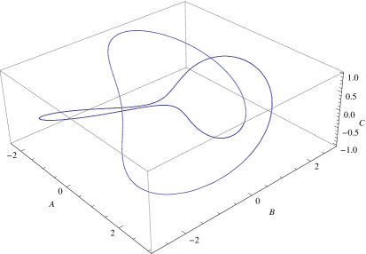
Figure 1: The trefoil knot for Eqs. (3.13)–(3.15), where $A_{0}=B_{0}=C_{0}=0$.

$$H_{1} = -2\tan(2\tau)-\frac{2\sin(3\tau)}{2+\cos(3\tau)},$$ (3.17)

$$H_{2} = -2\cot(2\tau)-\frac{2\sin(3\tau)}{2+\cos(3\tau)},$$ (3.18)

$$H_{3} = 3\cot(3\tau).$$ (3.19)

Figure 2: The evolution of the Hubble parameters for Eqs. (3.17)–(3.19).

In Fig.2 we plot the evolution of $H_{i}$ for the solution (3.17)–(3.19) with (3.16). It is interesting to study the evolution of the volume of the trefoil knot universe. For our case it is given by

$$V=[2+\cos(3\tau)]^{2}\cos(2\tau)\sin(2\tau)\sin(3\tau).$$ (3.20)

Figure 3: The evolution of the volume of the trefoil knot universe with respect to the cosmic time $\tau$ for Eq.(3.20).

In Fig. 3 we plot the evolution of the volume of the trefoil knot universe with respect to the cosmic time $\tau$ for Eq. (3.20) with (3.16). To get $V\geq 0$, we must consider $A_{0},B_{0},C_{0}>0$, if exactly e.g. as $A_{0}>3,B_{0}>3,C_{0}>1$. But below for simplicity we take the case (3.16). The other interesting quantity is the scalar curvature. For the trefoil knot solution (3.13)-(3.15), it has the form

$$R = (6(12\sin^{2}(3\tau)\sin^{2}(2\tau)-28\sin(3\tau)\cos(2\tau)\sin(2\tau)+3\sin^{3}(3\tau)\cos(2\tau)\sin(2\tau)-$$ (3.21)

$$-12\sin^{2}(3\tau)\cos^{2}(2\tau)-8\cos(3\tau)\sin^{2}(2\tau)-8\cos^{2}(3\tau)\sin^{2}(2\tau)-2\cos^{3}(3\tau)\sin^{2}(2\tau)+$$

$$+8\cos(3\tau)\cos^{2}(2\tau)+8\cos^{2}(3\tau)\cos^{2}(2\tau)+2\cos^{3}(3\tau)\cos^{2}(2\tau)-$$

$$-52\sin(3\tau)\cos(2\tau)\cos(3\tau)\sin(2\tau)-19\cos(2\tau)\sin(2\tau)\sin(3\tau)\cos^{2}(3\tau)+$$

$$+6\sin^{2}(2\tau)\sin^{2}(3\tau)\cos(3\tau)-$$

$$-6\cos^{2}(2\tau)\sin^{2}(3\tau)\cos(3\tau)))/(\sin(2\tau)\cos(2\tau)(2+\cos(3\tau))^{2}\sin(3\tau)).$$

Figure 4: The evolution of the $R$ with respect of the cosmic time $\tau$ for Eq.(3.21)

In Fig.4 we plot the evolution of the $R$ with respect of the cosmic time $\tau$.

So we have shown that the universe can live in the trefoil knot orbit according to the solution (3.13)-(3.15). It is interesting to note that this trefoil knot solution admits infinite number accelerated and decelerated expansion phases of the universe. To show this, as an example let us consider the solution for $C$ from (3.13)-(3.15) that is $C=C_{0}+\sin(3\tau)$. In this case we have $\ddot{C}=-9\sin(3\tau)$ so that $\ddot{C}>0$ (accelerating phase) as $\tau\in(\frac{\pi}{3}+\frac{2n\pi}{3},\frac{2\pi}{3}+\frac{2n\pi}{3})$ and $\ddot{C}<0$ (decelerating phase) as $\tau\in(\frac{2n\pi}{3},\frac{\pi}{3}+\frac{2n\pi}{3})$ with the transion points $\dot{C}=3\cos(3\tau_{i})=0$ as $\tau_{i}=(0.5\pi+n\pi)/3$, where $n$ is integer that is $n=0,\pm 1,\pm 2,\pm 3,...$.

3.2 Example 2.

Now we consider the following parametric EoS

$$p_{1} = -\frac{D_{1}}{E_{1}},$$ (3.22)

$$p_{2} = -\frac{D_{2}}{E_{2}},$$ (3.23)

$$p_{3} = -\frac{D_{3}}{E_{3}},$$ (3.24)

$$\rho = \frac{D_{0}}{E_{0}},$$ (3.25)

where

$$D_{1} = -\sin^{2}(2\tau)\cos^{2}(3\tau)+(-2\cos(2\tau)-4\sin^{2}(2\tau)-3-\sin(3\tau)\sin(2\tau))\cos(3\tau)+$$ (3.26)

$$+\sin(3\tau)\sin(2\tau)-4\cos(2\tau)-\sin^{2}(3\tau)-4\sin^{2}(2\tau),$$

$$E_{1} = 1,$$ (3.27)

$$D_{2} = -(2+\cos^{2}(3\tau))\cos^{2}(2\tau)-\sin(3\tau)(-1+\cos(3\tau))\cos(2\tau)+$$ (3.28)

$$+(-3+2\sin(2\tau))\cos(3\tau)+4\sin(2\tau)-\sin^{2}(3\tau),$$

$$E_{2} = 1,$$ (3.29)

$$D_{3} = -(2+\cos^{2}(3\tau))\cos^{2}(2\tau)+(-\sin(2\tau)\cos^{2}(3\tau)+(-4\sin(2\tau)-2)\cos(3\tau)+3\sin(3\tau)-$$ (3.30)

$$-4-4\sin(2\tau))\cos(2\tau)+2\sin(2\tau)\cos(3\tau)+(4+3\sin(3\tau))\sin(2\tau)-\sin^{2}(3\tau),$$

$$E_{3} = 1,$$ (3.31)

$$D_{0} = (2+\cos(3\tau))(((2+\cos(3\tau))\sin(2\tau)+\sin(3\tau))\cos(2\tau)+\sin(3\tau)\sin(2\tau)),$$ (3.32)

$$E_{0} = 1.$$ (3.33)

Substituting these expressions for the pressures and density of energy into the system (3.22)–(3.25), we obtain the following its solution

$$H_{1} = [2+\cos(3\tau)]\cos(2\tau)=2\cos(2\tau)+0.5[\cos(5\tau)+\cos(\tau)],$$ (3.34)

$$H_{2} = [2+\cos(3\tau)]\sin(2\tau)=2\sin(2\tau)+0.5[\sin(5\tau)-\sin(\tau)],$$ (3.35)

$$H_{3} = \sin(3\tau).$$ (3.36)

We see that this solution again describes the trefoil knot but for the ”coordinates” $H_{i}$. Note that the scale factors we can recovered from (2.17). We get

$$A = A_{0}e^{\sin(2\tau)+0.1\sin(5\tau)+0.5\sin(\tau)},$$ (3.37)

$$B = B_{0}e^{-[\cos(2\tau)+0.1\cos(5\tau)-0.5\cos(\tau)]},$$ (3.38)

$$C = C_{0}e^{-\frac{1}{3}\cos(3\tau)},$$ (3.39)

where $A_{0},B_{0},C_{0}$ are some real constants. In Fig.5 we plot the evolution of $A,B,C$ accordingly to (3.37)–(3.39) and for the initial conditions $A(0)=1,B(0)=e^{-0.6},C(0)=e^{-1/3}$, where we assume that $A_{0}=B_{0}=C_{0}=1$.

Figure 5: The evolution of $A,B,C$ accordingly to (3.37)–(3.39), [$t\in 0..2\pi$].

For this example, the volume of the universe is given by

$$V=V_{0}e^{\{\sin(2\tau)+0.1\sin(5\tau)+0.5\sin(\tau)-[\cos(2\tau)+0.1\cos(5\tau)-0.5\cos(\tau)]-\frac{1}{3}\cos(3\tau)\}}.$$ (3.40)

The evolution of the volume for (3.40) is presented in Fig. 6 for $A_{0}=B_{0}=C_{0}=V_{0}=1$ and for the intial condition $V(0)=e^{-14/15}$.

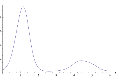
Figure 6: The evolution of the volume for (3.40) with $A_{0}=B_{0}=C_{0}=V_{0}=1$.

The scalar curvature has the form

$$R = (2\cos^{2}(2\tau)+2\sin^{2}(2\tau)+2\cos(2\tau)\sin(2\tau))\cos^{2}(3\tau)+(8\cos^{2}(2\tau)+(2\sin(3\tau)+4+$$ (3.41)

$$+8\sin(2\tau))\cos(2\tau)+6+8\sin^{2}(2\tau)+(-4+2\sin(3\tau))\sin(2\tau))\cos(3\tau)+8\cos^{2}(2\tau)+$$

$$+(-2\sin(3\tau)+8+8\sin(2\tau))\cos(2\tau)+8\sin^{2}(2\tau)+$$

$$+(-8-2\sin(3\tau))\sin(2\tau)+2\sin^{2}(3\tau).$$

Figure 7: The evolution of the $R$ with respect of the cosmic time $\tau$ for Eq.(3.41)

In Fig.7 we plot the evolution of the $R$ with respect of the cosmic time $\tau$. Finally we conclude that the Einstein equations for the Bianchi I type metric admit the trefoil knot solution of the form (3.34)-(3.36) or (3.37)-(3.39). These solutions describe the accelerated and decelerated phases of the expansion of the universe.

3.3 Example 3.

Now we present a new kind of the trefoil knot universes. Let the system (2.21)–(2.24) has the solution

$$A = A_{0}+[2+\mbox{cn}(3\tau)]\mbox{cn}(2\tau),$$ (3.42)

$$B = B_{0}+[2+\mbox{cn}(3\tau)]\mbox{sn}(2\tau),$$ (3.43)

$$C = C_{0}+\mbox{sn}(3\tau),$$ (3.44)

where $\mbox{cn}(t)\equiv\mbox{cn}(t,k)$ and $\mbox{sn}(t)\equiv\mbox{sn}(t,k)$ are the Jacobian elliptic functions which are doubly periodic functions, $k$ is the elliptic modulus. Fig. 8 shows the knotted closed curve corresponding to the solution (3.42)–(3.44) with (3.16). Substituting the formulas (3.42)–(3.44) into the system (2.21)–(2.24) we get the corresponding expressions for $\rho$ and $p_{i}$ that gives us the parametric EoS. This parametric EoS reads as

Figure 8: The knotted closed curve corresponding to the solution (3.42)–(3.44) with (3.16), $t\in[0,4\pi$], $k=1/3$.

$$p_{1} = -\frac{D_{1}}{E_{1}},$$ (3.45)

$$p_{2} = -\frac{D_{2}}{E_{2}},$$ (3.46)

$$p_{3} = -\frac{D_{3}}{E_{3}},$$ (3.47)

$$\rho = \frac{D_{0}}{E_{0}},$$ (3.48)

where

$$D_{1} = 9k^{2}cn(3\tau,k)sn^{3}(3\tau,k)sn(2\tau,k)-12\frac{\partial}{\partial\tau}am(3\tau,k)sn^{2}(3\tau,k)cn(2\tau,k)\frac{\partial}{\partial\tau}am(2\tau,k)-$$ (3.49)

$$-4sn(2\tau,k)((9/4)cn^{3}(3\tau,k)k^{2}+(9/2)cn^{2}(3\tau,k)k^{2}+$$

$$+((45/4)\frac{\partial}{\partial\tau}am^{2}(3\tau,k)+cn^{2}(2\tau,k)k^{2}+\frac{\partial}{\partial\tau}am^{2}(2\tau,k))cn(3\tau,k)+2\frac{\partial}{\partial\tau}am^{2}(2\tau,k)+$$

$$+(9/2)\frac{\partial}{\partial\tau}am^{2}(3\tau,k)+2cn^{2}(2\tau,k)k^{2})sn(3\tau,k)+18cn(3\tau,k)\frac{\partial}{\partial\tau}am(3\tau,k)$$

$$(2+cn(3\tau,k))cn(2\tau,k)\frac{\partial}{\partial\tau}am(2\tau,k),$$

$$E_{1} = (2+cn(3\tau,k))sn(2\tau,k)sn(3\tau,k),$$ (3.50)

$$D_{2} = 9k^{2}cn(3\tau,k)sn^{3}(3\tau,k)cn(2\tau,k)+12\frac{\partial}{\partial\tau}am(3\tau,k)sn^{2}(3\tau,k)\frac{\partial}{\partial\tau}am(2\tau,k)sn(2\tau,k)-$$ (3.51)

$$-9cn(2\tau,k)cn^{3}(3\tau,k)k^{2}+2cn^{2}(3\tau,k)k^{2}+((4/9)\frac{\partial}{\partial\tau}am^{2}(2\tau,k)+5\frac{\partial}{\partial\tau}am^{2}(3\tau,k)-$$

$$-(4/9)k^{2}sn^{2}(2\tau,k))cn(3\tau,k)+(8/9)\frac{\partial}{\partial\tau}am^{2}(2\tau,k)+2\frac{\partial}{\partial\tau}am^{2}(3\tau,k)-$$

$$-(8/9)k^{2}sn^{2}(2\tau,k))sn(3\tau,k)-$$

$$-18cn(3\tau,k)\frac{\partial}{\partial\tau}am(3\tau,k)(2+cn(3\tau,k))\frac{\partial}{\partial\tau}am(2\tau,k)sn(2\tau,k),$$

$$E_{2} = sn(3\tau,k)(2+cn(3\tau,k))cn(2\tau,k),$$ (3.52)

$$D_{3} = -4k^{2}sn(2\tau,k)(2+cn(3\tau,k))^{2}cn^{3}(2\tau,k)-30\frac{\partial}{\partial\tau}am(2\tau,k)sn(3\tau,k)\frac{\partial}{\partial\tau}am(3\tau,k)$$ (3.53)

$$(2+cn(3\tau,k))cn^{2}(2\tau,k)+4sn(2\tau,k)(k^{2}(2+cn^{2}(3\tau,k))sn^{2}(2\tau,k)+$$

$$+(-(9/2)\frac{\partial}{\partial\tau}am^{2}(3\tau,k)+(9/2)k^{2}sn^{2}(3\tau,k)-5\frac{\partial}{\partial\tau}am^{2}(2\tau,k))cn^{2}(3\tau,k)+$$

$$+(-20\frac{\partial}{\partial\tau}am^{2}(2\tau,k)+9k^{2}sn^{2}(3\tau,k)-9\frac{\partial}{\partial\tau}am^{2}(3\tau,k))cn(3\tau,k)+$$

$$+(27/4)sn^{2}(3\tau,k)\frac{\partial}{\partial\tau}am(3\tau,k)^{2}-20\frac{\partial}{\partial\tau}am^{2}(2\tau,k))cn(2\tau,k)+$$

$$+30\frac{\partial}{\partial\tau}am(3\tau,k)sn(3\tau,k)\frac{\partial}{\partial\tau}am(2\tau,k)sn^{2}(2\tau,k)(2+cn(3\tau,k)),$$

$$E_{3} = (2+cn(3\tau,k))^{2}cn(2\tau,k)sn(2\tau,k),$$ (3.54)

$$D_{0} = -4sn(3\tau,k)sn(2\tau,k)cn(2\tau,k)(2+cn(3\tau,k))^{2}\frac{\partial}{\partial\tau}am^{2}(2\tau,k)+6\frac{\partial}{\partial\tau}am(\tau,k)(2+cn(3\tau,k))$$ (3.55)

$$(cn^{2}(3\tau,k)+2cn(3\tau,k)-sn^{2}(3\tau,k))(cn(2\tau,k)-sn(2\tau,k))(cn(2\tau,k)+sn(2\tau,k))$$

$$\frac{\partial}{\partial\tau}am(2\tau,k)-18sn(3\tau,k)sn(2\tau,k)(-(1/2)sn^{2}(3\tau,k)+cn^{2}(3\tau,k)+$$

$$+2cn(3\tau,k))cn(2\tau,k)\frac{\partial}{\partial\tau}am^{2}(3\tau,k),$$

$$E_{0} = (2+cn^{2}(3\tau,k))cn(2\tau,k)sn(2\tau,k)sn(3\tau,k).$$ (3.56)

The volume of the universe for the solution (3.42)–(3.44) with (3.16) looks like

$$V=[2+\mbox{cn}(3\tau)]^{2}\mbox{cn}(2\tau)\mbox{sn}(2\tau)\mbox{sn}(3\tau).$$ (3.57)

The evolution of the volume for (3.57) is presented in Fig.9

Figure 9: The evolution of the volume of the trefoil knot universe with respect to the cosmic time $\tau$ for Eq.(3.57)

The scalar curvature has the form

$$R = (-8\mbox{sn}(2\tau,k)\mbox{sn}(3\tau,k)k^{2}(2+\mbox{cn}(3\tau,k))^{2}\mbox{cn}^{3}(2\tau,k)+$$ (3.58)

$$+12\mbox{dn}(2\tau,k)\mbox{dn}(3\tau,k)(2+\mbox{cn}(3\tau,k))(\mbox{cn}^{2}(3\tau,k)+$$

$$+2\mbox{cn}(3\tau,k)-3\mbox{sn}^{2}(3\tau,k))\mbox{cn}^{2}(2\tau,k)-18\mbox{sn}(3\tau,k)(-(4/9)k^{2}(2+\mbox{cn}(3\tau,k))^{2}\mbox{sn}^{2}(2\tau,k)+$$

$$+(-4k^{2}\mbox{cn}(3\tau,k)-2\mbox{cn}^{2}(3\tau,k)k^{2}-\mbox{dn}^{2}(3\tau,k))\mbox{sn}^{2}(3\tau,k)+$$

$$+(2+\mbox{cn}(3\tau,k))(\mbox{cn}^{3}(3\tau,k)k^{2}+2\mbox{cn}^{2}(3\tau,k)k^{2}+$$

$$+(5\mbox{dn}^{2}(3\tau,k)+(4/3)\mbox{dn}^{2}(2\tau,k))\mbox{cn}(3\tau,k)+$$

$$+(8/3)\mbox{dn}^{2}(2\tau,k)+2\mbox{dn}^{2}(3\tau,k)))\mbox{sn}(2\tau,k)\mbox{cn}(2\tau,k)-$$

$$-12\mbox{dn}(2\tau,k)\mbox{sn}^{2}(2\tau,k)\mbox{dn}(3\tau,k)(2+\mbox{cn}(3\tau,k))(\mbox{cn}^{2}(3\tau,k)+$$

$$+2\mbox{cn}(3\tau,k)-3\mbox{sn}^{2}(3\tau,k)))/(\mbox{cn}(2\tau,k)\mbox{sn}(2\tau,k)(2+\mbox{cn}(3\tau,k))^{2}\mbox{sn}(3\tau,k)).$$

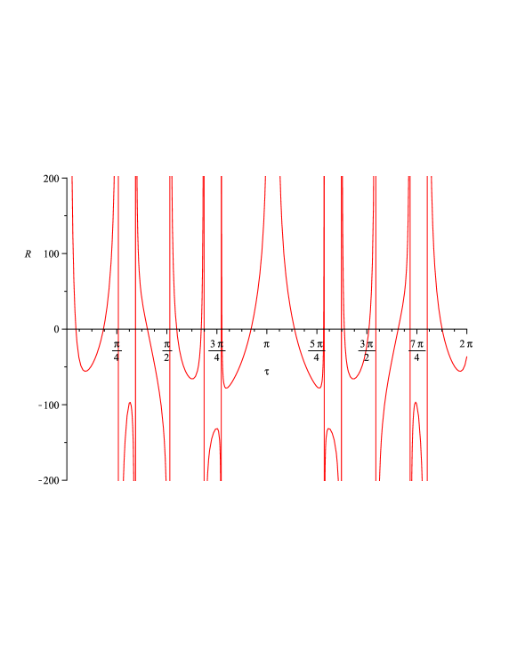
Figure 10: The evolution of the $R$ with respect of the cosmic time $\tau$ for Eq.(3.58)

In Fig.10 we plot the evolution of the $R$ with respect of the cosmic time $\tau$.

3.4 Example 4.

Our fourth example is given by

$$H_{1} = [2+\mbox{cn}(3\tau)]\mbox{cn}(2\tau),$$ (3.59)

$$H_{2} = [2+\mbox{cn}(3\tau)]\mbox{sn}(2\tau),$$ (3.60)

$$H_{3} = \mbox{sn}(3\tau)$$ (3.61)

which again the knotted closed curve in Fig. 8 but for the ”coordinates” $H_{i}$. Note that the corresponding parametric EoS looks like

$$p_{1} = -\frac{D_{1}}{E_{1}},$$ (3.62)

$$p_{2} = -\frac{D_{2}}{E_{2}},$$ (3.63)

$$p_{3} = -\frac{D_{3}}{E_{3}},$$ (3.64)

$$\rho = \frac{D_{0}}{E_{0}},$$ (3.65)

where

$$D_{1} = -(2+cn(3\tau,k))^{2}sn^{2}(2\tau,k)-sn(3\tau,k)(-3\frac{\partial}{\partial\tau}am(3\tau,k)+2+cn(3\tau,k))sn(2\tau,k)+$$ (3.66)

$$+(-2cn(2\tau,k)\frac{\partial}{\partial\tau}am(2\tau,k)-3\frac{\partial}{\partial\tau}am(3\tau,k))cn(3\tau,k)-4cn(2\tau,k)\frac{\partial}{\partial\tau}am(2\tau,k)-$$

$$-sn^{2}(3\tau,k),$$

$$E_{1} = 1,$$ (3.67)

$$D_{2} = -(2+cn(3\tau,k))^{2}cn^{2}(2\tau,k)-sn(3\tau,k)(-3\frac{\partial}{\partial\tau}am(3\tau,k)+2+cn(3\tau,k))cn(2\tau,k)+$$ (3.68)

$$+(-3\frac{\partial}{\partial\tau}am(3\tau,k)+2\frac{\partial}{\partial\tau}am(2\tau,k)sn(2\tau,k))cn(3\tau,k)+4\frac{\partial}{\partial\tau}am(2\tau,k)sn(2\tau,k)-$$

$$-sn^{2}(3\tau,k),$$

$$E_{2} = 1,$$ (3.69)

$$D_{3} = -(2+cn(3\tau,k))^{2}cn^{2}(2\tau,k)+(-sn(2\tau,k)cn^{2}(3\tau,k)+(-4sn(2\tau,k)-2\frac{\partial}{\partial\tau}am(2\tau,k))$$ (3.70)

$$cn(3\tau,k)+3sn(3\tau,k)\frac{\partial}{\partial\tau}am(3\tau,k)-4\frac{\partial}{\partial\tau}am(2\tau,k)-4sn(2\tau,k))cn(2\tau,k)+$$

$$+2\frac{\partial}{\partial\tau}am(2\tau,k)sn(2\tau,k)cn(3\tau,k)+(4\frac{\partial}{\partial\tau}am(2\tau,k)+3sn(3\tau,k)\frac{\partial}{\partial\tau}am(3\tau,k))sn(2\tau,k)-$$

$$-sn^{2}(3\tau,k),$$

$$E_{3} = 1,$$ (3.71)

$$D_{0} = (((2+cn(3\tau,k))sn(2\tau,k)+sn(3\tau,k))cn(2\tau,k)+sn(2\tau,k)sn(3\tau,k))$$ (3.72)

$$(2+cn(3\tau,k)),$$

$$E_{0} = 1.$$ (3.73)

Figure 11: The evolution of $p_{i},\rho$ for (3.62)–(3.65), $t\in[0,2\pi$], $k=1/3$, $\rho$(red), $p_{1}$(blue), $p_{2}$(green), $p_{3}$(black).

In Fig. 11 we plot the evolution of $p_{i},\rho$ for (3.62)–(3.65). The scalar curvature has the form

$$R = 2(2+\mbox{cn}(3\tau,k))^{2}\mbox{cn}^{2}(2\tau,k)+(2\mbox{sn}(2\tau,k)\mbox{cn}^{2}(3\tau,k)+(8\mbox{sn}(2\tau,k)+4\mbox{dn}(2\tau,k)+$$ (3.74)

$$+2\mbox{sn}(3\tau,k))\mbox{cn}(3\tau,k)+8\mbox{sn}(2\tau,k)+(4-6\mbox{dn}(3\tau,k))\mbox{sn}(3\tau,k)+$$

$$+8\mbox{dn}(2\tau,k))\mbox{cn}(2\tau,k)+2\mbox{sn}^{2}(2\tau,k)\mbox{cn}^{2}(3\tau,k)+(8\mbox{sn}^{2}(2\tau,k)+$$

$$+(-4\mbox{dn}(2\tau,k)+2\mbox{sn}(3\tau,k))\mbox{sn}(2\tau,k)+6\mbox{dn}(3\tau,k))\mbox{cn}(3\tau,k)+$$

$$+8\mbox{sn}^{2}(2\tau,k)+((4-6\mbox{dn}(3\tau,k))\mbox{sn}(3\tau,k)-8\mbox{dn}(2\tau,k))\mbox{sn}(2\tau,k)+2\mbox{sn}(3\tau,k)^{2}$$

Figure 12: The evolution of the $R$ with respect of the cosmic time $\tau$ for Eq.(3.74)

In Fig.12 we plot the evolution of the $R$ with respect of the cosmic time $\tau$.

4 The figure-eight knot universe

Our aim in this section is to demonstrate some examples the figure-eight knot universes for the Bianchi type I metric (2.6). We give some particular figure-eight knot universe models.

4.1 Example 1.

Again, let us we assume that our universe is filled by the fluid with the following parametric EoS

$$\rho = \frac{D_{8}}{E_{8}},$$ (4.1)

$$p_{1} = -\frac{D_{9}}{E_{9}},$$ (4.2)

$$p_{2} = -\frac{D_{10}}{E_{10}},$$ (4.3)

$$p_{3} = -\frac{D_{11}}{E_{11}},$$ (4.4)

where

$$D_{8} = (-2\sin(2\tau)\cos(3\tau)-(3(2+\cos(2\tau)))\sin(3\tau))(-2\sin(2\tau)\sin(3\tau)+$$ (4.5)

$$(3(2+\cos(2\tau)))\cos(3\tau))\sin(4\tau)+12\cos(3\tau)((2+\cos(2\tau))\cos(3\tau)-$$

$$(2/3)\sin(2\tau)\sin(3\tau))(2+\cos(2\tau))\cos(4\tau)-(12(2+\cos(2\tau)))\cos(4\tau)*$$

$$((2+\cos(2\tau))\sin(3\tau)+(2/3)\sin(2\tau)\cos(3\tau))\sin(3\tau),$$

$$E_{8} = (2+\cos(2\tau))^{2}\cos(3\tau)\sin(3\tau)\sin(4\tau),$$ (4.6)

$$D_{9} = ((72+36\cos(2\tau))\cos(4\tau)-12\sin(4\tau)\sin(2\tau))\cos(3\tau)-(29((24/29)*$$ (4.7)

$$\cos(4\tau)\sin(2\tau)+(cos(2\tau)+50/29)\sin(4\tau)))\sin(3\tau),$$

$$E_{9} = \sin(4\tau)(2+\cos(2\tau))\sin(3\tau),$$ (4.8)

$$D_{10} = (-24\cos(4\tau)\sin(2\tau)+\sin(4\tau)(-29\cos(2\tau)-50))\cos(3\tau)-$$ (4.9)

$$(36((2+\cos(2\tau))\cos(4\tau)-(1/3)\sin(4\tau)\sin(2\tau)))\sin(3\tau),$$

$$E_{10} = \sin(4\tau)(2+\cos(2\tau))\cos(3\tau),$$ (4.10)

$$D_{11} = -(30(2+\cos(2\tau)))\sin(2\tau)\cos(3\tau)^{2}+\sin(3\tau)(12\sin(2\tau)^{2}-196\cos(2\tau)-$$ (4.11)

$$180-53\cos(2\tau)^{2})\cos(3\tau)+30\sin(2\tau)\sin(3\tau)^{2}(2+\cos(2\tau)),$$

$$E_{11} = (2+\cos(2\tau))^{2}\cos(3\tau)\sin(3\tau).$$ (4.12)

Substituting these expressions for the pressuries and the density of energy into the system (2.21)–(2.24), we obtain the following its solution [30]

$$A = A_{0}+[2+\cos(2\tau)]\cos(3\tau),$$ (4.13)

$$B = B_{0}+[2+\cos(2\tau)]\sin(3\tau),$$ (4.14)

$$C = C_{0}+\sin(4\tau).$$ (4.15)

This solution is nothing but the parametric equation of the figure-eight knot as we can see from Fig. 13, where we assume that $A_{0}=B_{0}=C_{0}=0$ and the initial conditions have the form $A(0)=3,B(0)=0,C(0)=0$. And for that reason in [30] we called such models as the figure-eight knot universes.

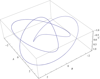
Figure 13: The figure-eight knot for (4.13)–(4.15) with (3.16).

Note that the ”coordinates” $A,B,C$ with (3.16) satisfy the equation

$$4(h-2)^{4}-4(h-2)^{2}+z^{2}=0,$$ (4.16)

where $h=2+\cos(2\tau)$. Let us calculate the volume of the universe. For our case it is given by

$$V=[2+\cos(2\tau)]^{2}\cos(3\tau)\sin(3\tau)\sin(4\tau),$$ (4.17)

where we used (3.16).

Figure 14: The evolution of the volume for the solution (4.13)–(4.15) with (3.16), $t\in[0,2\pi$].

In Fig.9 we present the evolution of the volume for the solution (4.13)–(4.15) with (3.16). The scalar curvature has the form

$$R = ((24(\cos(4\tau)\cos(2\tau)-(3/2)\sin(4\tau)\sin(2\tau)+2\cos(4\tau)))(2+\cos(2\tau))\cos^{2}(3\tau)-$$ (4.18)

$$-102\sin(3\tau)(\sin(4\tau)\cos^{2}(2\tau)+((188/51)\sin(4\tau)+(16/51)\cos(4\tau)\sin(2\tau))\cos(2\tau)+$$

$$+(32/51)\cos(4\tau)\sin(2\tau)+(172/51)\sin(4\tau)-$$

$$-(4/51)\sin^{2}(2\tau)\sin(4\tau))\cos(3\tau)-24\sin^{2}(3\tau)(\cos(4\tau)\cos(2\tau)-$$

$$-(3/2)\sin(4\tau)\sin(2\tau)+2\cos(4\tau))(2+\cos(2\tau)))/(\sin(3\tau)\cos(3\tau)*$$

$$*(2+\cos(2\tau))^{2}\sin(4\tau)).$$

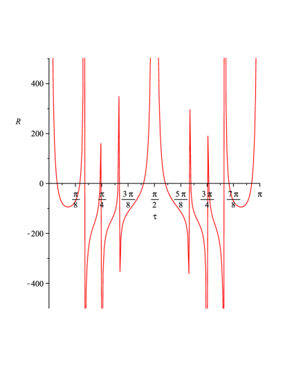
Figure 15: The evolution of the $R$ with respect of the cosmic time $\tau$ for Eq.(4.18)

In Fig.15 we plot the evolution of the $R$ with respect of the cosmic time $\tau$. So we found the figure-eight knot solution of the Einstein equations which again describe the accelerated and decelerated expansion phases of the universe.

4.2 Example 2

Now we consider the system (2.25)–(2.28). Let its solution is given by

$$H_{1} = [2+\cos(2\tau)]\cos(3\tau)=2\cos(3\tau)+\cos(5\tau)+\cos(\tau),$$ (4.19)

$$H_{2} = [2+\cos(2\tau)]\sin(3\tau)=2\sin(3\tau)+\sin(\tau)+\sin(5\tau),$$ (4.20)

$$H_{3} = \sin(4\tau).$$ (4.21)

Then the coorresponding scale factors read as

$$A = A_{0}e^{\frac{2}{3}\sin(3\tau)+0.2\sin(5\tau)+\sin(\tau)},$$ (4.22)

$$B = B_{0}e^{-[\frac{2}{3}\cos(3\tau)+0.2cos(5\tau)+\cos(\tau)]},$$ (4.23)

$$C = C_{0}e^{-0.25\cos(4\tau)}.$$ (4.24)

For this solution the parametric EoS looks like

$$\rho = \frac{D_{0}}{E_{0}},$$ (4.25)

$$p_{1} = -\frac{D_{1}}{E_{1}},$$ (4.26)

$$p_{2} = -\frac{D_{2}}{E_{2}},$$ (4.27)

$$p_{3} = -\frac{D_{3}}{E_{3}},$$ (4.28)

where

$$D_{0} = (((2+\cos(2\tau))\sin(3\tau)+\sin(4\tau))\cos(3\tau)+\sin(3\tau)\sin(4\tau))(2+\cos(2\tau)),$$ (4.29)

$$E_{0} = 1,$$ (4.30)

$$D_{1} = -(2+\cos(2\tau))^{2}\sin^{2}(3\tau)+(2\sin(2\tau)-2\sin(4\tau)-\sin(4\tau)\cos(2\tau))\sin(3\tau)-$$ (4.31)

$$-6\cos(3\tau)-3\cos(3\tau)\cos(2\tau)-4\cos(4\tau)-\sin^{2}(4\tau),$$

$$E_{1} = 1,$$ (4.32)

$$D_{2} = -(2+\cos(2\tau))^{2}\cos^{2}(3\tau)+(2\sin(2\tau)-2\sin(4\tau)-\sin(4\tau)\cos(2\tau))\cos(3\tau)-$$ (4.33)

$$-4\cos(4\tau)+6\sin(3\tau)+3\sin(3\tau)\cos(2\tau)-\sin^{2}(4\tau),$$

$$E_{2} = 1,$$ (4.34)

$$D_{3} = -3\sin(\tau)-64\sin(\tau)\cos^{9}(\tau)+36\sin(\tau)\cos^{5}(\tau)+40\sin(\tau)\cos^{4}(\tau)+4\sin(\tau)\cos^{3}(\tau)-$$ (4.35)

$$-6\sin(\tau)\cos^{2}(\tau)-3\sin(\tau)\cos(\tau)-25\cos^{2}(\tau)+5\cos(\tau)-40\cos^{5}(\tau)-64\cos^{1}0(\tau)+$$

$$+96\cos^{8}(\tau)-84\cos^{6}(\tau)+68\cos^{4}(\tau)+26\cos^{3}(\tau),$$

$$E_{3} = 1.$$ (4.36)

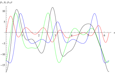
Figure 16: The plot of the EoS (4.25)–(4.28), $t\in[0,2\pi$], $\rho$(red), $p_{1}$(blue), $p_{2}$(green), $p_{3}$(black).

In Fig. 16 we plot the EoS (4.25)–(4.28). For this example, the evolution of the volume of the universe is given by

$$V=V_{0}e^{\frac{2}{3}\sin(3\tau)+0.2\sin(5\tau)+\sin(\tau)-\frac{2}{3}\cos(3\tau)-0.2cos(5\tau)-\cos(\tau)-0.25\cos(4\tau)}.$$ (4.37)

The evolution of the volume is presented in Fig.17 for $A_{0}=B_{0}=C_{0}=V_{0}=1$ and for the intial condition $V(0)=e^{-127/60}$.

Figure 17: The evolution of the volume for the expression (4.37) with $V_{0}=1$, $t\in[0,2\pi$].

The scalar curvature has the form

$$R = 2(2+\cos(2\tau))^{2}\cos^{2}(3\tau)+(2(2+\cos(2\tau))^{2}\sin(3\tau)+(6+2\sin(4\tau))\cos(2\tau)+$$ (4.38)

$$+12-4\sin(2\tau)+4\sin(4\tau))\cos(3\tau)+2(2+\cos(2\tau))^{2}\sin^{2}(3\tau)+$$

$$+((-6+2\sin(4\tau))\cos(2\tau)+4\sin(4\tau)-4\sin(2\tau)-12)*$$

$$*\sin(3\tau)+2\sin^{2}(4\tau)+8\cos(4\tau).$$

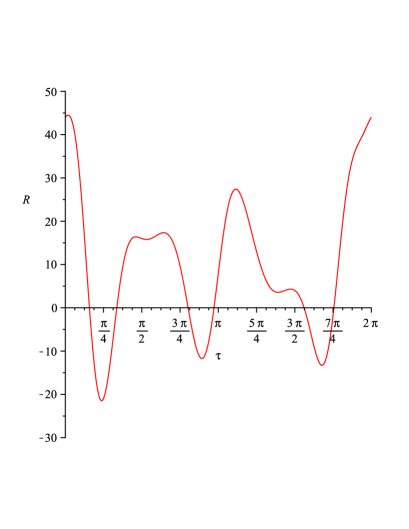
Figure 18: The evolution of the $R$ with respect of the cosmic time $\tau$ for Eq.(4.38)

In Fig.18 we plot the evolution of the $R$ with respect of the cosmic time $\tau$. Again we have shown that the Einstein equations admit the figure-eight knot solution and it again describe the accelerated and decelerated expansion phases of the universe.

4.3 Example 3.

Now we present the figure-eight knot universe induced by the Jacobian elliptic functions. Let the system (2.21)–(2.24) has the solution

$$A = A_{0}+[2+\mbox{cn}(2\tau)]\mbox{cn}(3\tau),$$ (4.39)

$$B = B_{0}+[2+\mbox{cn}(2\tau)]\mbox{sn}(3\tau),$$ (4.40)

$$C = C_{0}+\mbox{sn}(4\tau).$$ (4.41)

Figure 19: The knotted closed curve corresponding to the solution (4.39)–(4.41) with (3.16), $t\in[0,4\pi$], $k=1/3$.

Note that $\mbox{cn}(t)$ and $\mbox{sn}(t)$ are the doubly periodic Jacobian elliptic functions. Fig.19 shows the knotted closed curve corresponding to the solution (4.39)–(4.41) with (3.16). Substituting the formulas (4.39)–(4.41) into the system (2.21)–(2.24) we get the corresponding expressions for $\rho$ and $p_{i}$ that gives us the parametric EoS. The evolution of the volume of the universe for (3.16) reads as

$$V=[2+\mbox{cn}(2\tau)]^{2}\mbox{cn}(3\tau)\mbox{sn}(3\tau)\mbox{sn}(4\tau).$$ (4.42)

The scalar curvature has the form

$$R = (-18\mbox{sn}(3\tau,k)\mbox{sn}(4\tau,k)k^{2}(2+\mbox{cn}(2\tau,k))^{2}\mbox{cn}^{3}(3\tau,k)+(24(-(3/2)\mbox{sn}(2\tau,k)\mbox{dn}(2\tau,k)\mbox{sn}(4\tau,k)+$$ (4.43)

$$+\mbox{cn}(4\tau,k)\mbox{dn}(4\tau,k)(2+\mbox{cn}(2\tau,k))))(2+\mbox{cn}(2\tau,k))\mbox{dn}(3\tau,k)\mbox{cn}^{2}(3\tau,k)-$$

$$-(32(-(9/16)\mbox{sn}(4\tau,k)k^{2}(2+\mbox{cn}(2\tau,k))^{2}\mbox{sn}^{2}(3\tau,k)+((\mbox{cn}^{2}(4\tau,k)k^{2}+(27/16)\mbox{dn}^{2}(3\tau,k)+$$

$$+\mbox{dn}^{2}(4\tau,k)-(1/2)k^{2}\mbox{sn}^{2}(2\tau,k)+(1/2)\mbox{dn}^{2}(2\tau,k))\mbox{cn}^{2}(2\tau,k)+(-k^{2}\mbox{sn}^{2}(2\tau,k)+$$

$$+(27/4)\mbox{dn}^{2}(3\tau,k)+\mbox{dn}^{2}(2\tau,k)+4\mbox{dn}^{2}(4\tau,k)+4\mbox{cn}^{2}(4\tau,k)k^{2})\mbox{cn}(2\tau,k)+4\mbox{dn}^{2}(4\tau,k)+$$

$$+(27/4)\mbox{dn}^{2}(3\tau,k)-(1/4)\mbox{dn}^{2}(2\tau,k)\mbox{sn}^{2}(2\tau,k)+4\mbox{cn}^{2}(4\tau,k)k^{2})\mbox{sn}(4\tau,k)+\mbox{cn}(4\tau,k)\mbox{dn}(4\tau,k)$$

$$\mbox{dn}(2\tau,k)\mbox{sn}(2\tau,k)(2+\mbox{cn}(2\tau,k))))\mbox{sn}(3\tau,k)\mbox{cn}(3\tau,k)-(24(-(3/2)\mbox{sn}(2\tau,k)\mbox{dn}(2\tau,k)$$

$$\mbox{sn}(4\tau,k)+\mbox{cn}(4\tau,k)\mbox{dn}(4\tau,k)(2+\mbox{cn}(2\tau,k))))(2+\mbox{cn}(2\tau,k))\mbox{sn}^{2}(3\tau,k)\mbox{dn}(3\tau,k))/(\mbox{cn}(3\tau,k)$$

$$\mbox{sn}(3\tau,k)(2+\mbox{cn}(2\tau,k))^{2}\mbox{sn}(4\tau,k)).$$

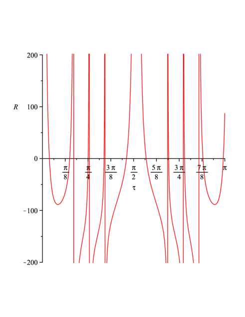
Figure 20: The evolution of the $R$ with respect of the cosmic time $\tau$ for Eq.(4.43)

In Fig.20 we plot the evolution of the $R$ with respect of the cosmic time $\tau$.

4.4 Example 4.

We now consider the following solution of the system (2.25)–(2.28):

$$H_{1} = [2+\mbox{cn}(2\tau)]\mbox{cn}(3\tau),$$ (4.44)

$$H_{2} = [2+\mbox{cn}(2\tau)]\mbox{sn}(3\tau),$$ (4.45)

$$H_{3} = \mbox{sn}(4\tau)$$ (4.46)

which again the trefoil knot universe as shown in Fig.19 but for the ”coordinates” $H_{i}$. The corresponding parametric EoS reads as

$$\rho = \frac{D_{0}}{E_{0}},$$ (4.47)

$$p_{1} = -\frac{D_{1}}{E_{1}},$$ (4.48)

$$p_{2} = -\frac{D_{2}}{E_{2}},$$ (4.49)

$$p_{3} = -\frac{D_{3}}{E_{3}},$$ (4.50)

where

$$D_{0} = (((2+cn(2\tau,k))sn(3\tau,k)+sn(4\tau,k))cn(3\tau,k)+sn(3\tau,k)sn(4\tau,k))$$ (4.51)

$$(2+cn(2\tau,k)),$$

$$E_{0} = 1,$$ (4.52)

$$D_{1} = 2\frac{\partial}{\partial\tau}am(2\tau,k)sn(2\tau,k)sn(3\tau,k)-(3(2+cn(2\tau,k)))cn(3\tau,k)\frac{\partial}{\partial\tau}am(3\tau,k)-$$ (4.53)

$$-4cn(4\tau,k)\frac{\partial}{\partial\tau}am(4\tau,k)-(2+cn(2\tau,k))^{2}sn(3\tau,k)^{2}-sn(4\tau,k)^{2}-$$

$$-(2+cn(2\tau,k))sn(3\tau,k)sn(4\tau,k),$$

$$E_{1} = 1,$$ (4.54)

$$D_{2} = -4cn(4\tau,k)\frac{\partial}{\partial\tau}am(4\tau,k)+2\frac{\partial}{\partial\tau}am(2\tau,k)sn(2\tau,k)cn(3\tau,k)+(3(2+cn(2\tau,k)))$$ (4.55)

$$\frac{\partial}{\partial\tau}am(3\tau,k)sn(3\tau,k)-sn^{2}(4\tau,k)-(2+cn(2\tau,k))^{2}cn^{2}(3\tau,k)-$$

$$-(2+cn(2\tau,k))cn(3\tau,k)sn(4\tau,k),$$

$$E_{2} = 1,$$ (4.56)

$$D_{3} = -(2+cn(2\tau,k))^{2}cn^{2}(3\tau,k)+(-sn(3\tau,k)cn^{2}(2\tau,k)+(-4sn(3\tau,k)-$$ (4.57)

$$-3\frac{\partial}{\partial\tau}am(3\tau,k))cn(2\tau,k)+2\frac{\partial}{\partial\tau}am(2\tau,k)sn(2\tau,k)-6\frac{\partial}{\partial\tau}am(3\tau,k)-$$

$$-4sn(3\tau,k))cn(3\tau,k)+3\frac{\partial}{\partial\tau}am(3\tau,k)sn(3\tau,k)cn(2\tau,k)+$$

$$+(6\frac{\partial}{\partial\tau}am(3\tau,k)+2\frac{\partial}{\partial\tau}am(2\tau,k)sn(2\tau,k))sn(3\tau,k)-sn^{2}(4\tau,k),$$

$$E_{3} = 1.$$ (4.58)

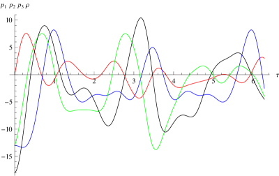
Figure 21: The plot of the EoS (4.47)–(4.50), $t\in[0,2\pi$], $k=1/3$, $\rho$(red), $p_{1}$(blue), $p_{2}$(green), $p_{3}$(black).

Its plot we give in Fig.21.

The scalar curvature has the form

$$R = 2(2+\mbox{cn}(2\tau,k))^{2}\mbox{cn}(3\tau,k)^{2}+(2(2+\mbox{cn}(2\tau,k))^{2}\mbox{sn}(3\tau,k)+(6\mbox{dn}(3\tau,k)+2\mbox{sn}(4\tau,k))\mbox{cn}(2\tau,k)+$$ (4.59)

$$+12\mbox{dn}(3\tau,k)-4\mbox{dn}(2\tau,k)\mbox{sn}(2\tau,k)+4\mbox{sn}(4\tau,k))\mbox{cn}(3\tau,k)+2(2+\mbox{cn}(2\tau,k))^{2}\mbox{sn}(3\tau,k)^{2}+$$

$$+((-6\mbox{dn}(3\tau,k)+2\mbox{sn}(4\tau,k))\mbox{cn}(2\tau,k)+4\mbox{sn}(4\tau,k)-4\mbox{dn}(2\tau,k)\mbox{sn}(2\tau,k)-12\mbox{dn}(3\tau,k))*$$

$$*\mbox{sn}(3\tau,k)+2\mbox{sn}(4\tau,k)^{2}+8\mbox{cn}(4\tau,k)\mbox{dn}(4\tau,k).$$

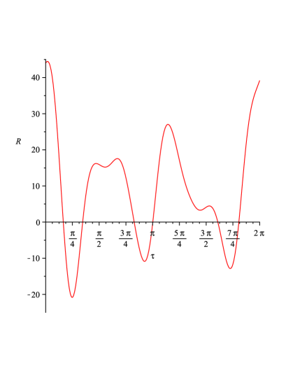
Figure 22: The evolution of the $R$ with respect of the cosmic time $\tau$ for Eq.(4.59)

In Fig.22 we plot the evolution of the $R$ with respect of the cosmic time $\tau$.

5 Other unknotted models of the universe

In this section we would like to present some unknotted but closed curve solutions of the Einstein equation for the Bianchi I type metric. As an examples we consider the spiky and Mobious strip universe solutions.

5.1 Spiky universe solutions

Our aim in this subsection is to present some unknotted closed curve solutions namely the spiky universe solutions.

5.1.1 Example 1

Let our universe is filled by the fluid with the following parametric EoS

$$\rho = \frac{D_{8}}{E_{8}},$$ (5.1)

$$p_{1} = -\frac{D_{9}}{E_{9}},$$ (5.2)

$$p_{2} = -\frac{D_{10}}{E_{10}},$$ (5.3)

$$p_{3} = -\frac{D_{11}}{E_{11}},$$ (5.4)

where

$$D_{8} = -[\alpha\sin((n-1)\tau)(n-1)+\alpha(n-1)\sin(\tau)][\alpha\cos((n-1)\tau)(n-1)-$$ (5.5)

$$\alpha(n-1)\cos(\tau)]\sin(\tau)+[\alpha\cos((n-1)\tau)(n-1)-\alpha(n-1)\cos(\tau)]\cos(\tau)\times$$

$$[\alpha\cos((n-1)\tau)+\alpha(n-1)\cos(\tau)]-[\alpha\sin((n-1)\tau)(n-1)+\alpha(n-1)\sin(\tau)]\times$$

$$[\alpha\sin((n-1)\tau)-\alpha(n-1)\sin(\tau)]\cos(\tau),$$

$$E_{8} = [\alpha\cos((n-1)\tau)+\alpha(n-1)\cos(\tau)][\alpha\sin((n-1)\tau)-\alpha(n-1)\sin(\tau)]\sin(\tau),$$ (5.6)

$$D_{9} = [-\alpha\sin((n-1)\tau)(n-1)^{2}+\alpha(n-1)\sin(\tau)]\sin(\tau)-[\alpha\sin((n-1)\tau)-\alpha(n-1)\sin(\tau)]\sin(\tau)+$$ (5.7)

$$[\alpha\cos((n-1)\tau)(n-1)-\alpha(n-1)\cos(\tau)]\cos(\tau),$$

$$E_{9} = [\alpha\sin((n-1)\tau)-\alpha(n-1)\sin(\tau)]\sin(\tau),$$ (5.8)

$$D_{10} = [\alpha\cos((n-1)\tau)+\alpha(n-1)\cos(\tau)]\sin(\tau)+\sin(\tau)[\alpha\cos((n-1)\tau)(n-1)^{2}+\alpha(n-1)\cos(\tau)]+$$ (5.9)

$$[\alpha\sin((n-1)\tau)(n-1)+\alpha(n-1)\sin(\tau)]\cos(\tau),$$

$$E_{10} = -[\alpha\cos((n-1)\tau)+\alpha(n-1)\cos(\tau)]\sin(\tau),$$ (5.10)

$$D_{11} = [\alpha\sin((n-1)\tau)-\alpha(n-1)\sin(\tau)][-\alpha\cos((n-1)\tau)(n-1)^{2}-\alpha(n-1)\cos(\tau)]+$$ (5.11)

$$[\alpha\cos((n-1)\tau)+\alpha(n-1)\cos(\tau)][-\alpha\sin((n-1)\tau)(n-1)^{2}+\alpha(n-1)\sin(\tau)]-$$

$$[\alpha\sin((n-1)\tau)(n-1)+\alpha(n-1)\sin(\tau)][\alpha\cos((n-1)\tau)(n-1)-\alpha(n-1)\cos(\tau)],$$

$$E_{11} = [\alpha\cos((n-1)\tau)+\alpha(n-1)\cos(\tau)][\alpha\sin((n-1)\tau)-\alpha(n-1)\sin(\tau)].$$ (5.12)

Substituting these expressions for the pressuries and the density of energy into the system (2.21)–(2.24), we obtain the following its solution

$$A = \alpha\cos[(n-1)\tau]+\alpha(n-1)\cos[\tau],$$ (5.13)

$$B = \alpha\sin[(n-1)\tau]-\alpha(n-1)\sin[\tau],$$ (5.14)

$$C = \sin(\tau).$$ (5.15)

It is the spiky like solution so that such solutions we call the spike universe. Its plot presented in Fig.23 for the initial conditions $A(0)=\alpha n=10,B(0)=0,C(0)=0$.

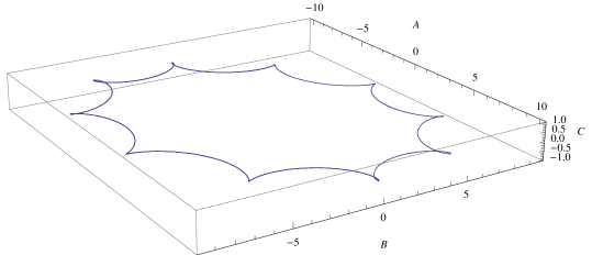
Figure 23: The spiky universe for (5.13)–(5.15), $n=10,\alpha=1$.

Let us calculate the volume of this universe. It is given by

$$V=\alpha^{2}[\cos[(n-1)\tau]+(n-1)\cos[\tau]][\sin[(n-1)\tau]-(n-1)\sin[\tau]]\sin(\tau).$$ (5.16)

In Fig.24 shown the evolution of the volume for (5.16), $n=10,\alpha=1$.

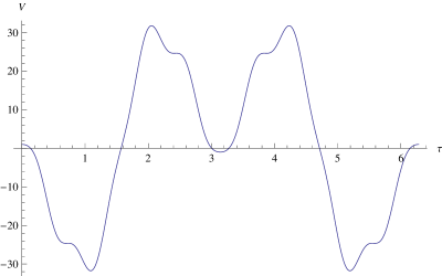
Figure 24: The evolution of the volume for (5.16), $n=10$, $\alpha=1$.

The scalar curvature has the form

$$R = (-2\cos(\tau)(n-1)\cos^{2}((n-1)\tau)+((6(4/3-2n+n^{2}))\sin(\tau)\sin((n-1)\tau)-$$ (5.17)

$$-(2((n-2)\cos(\tau)^{2}+\sin^{2}(\tau)(n^{2}-3n+4)))(n-1))\cos((n-1)\tau)+2\cos(\tau)(\sin^{2}((n-1)\tau)+$$

$$+\sin(\tau)(n^{2}-4n+6)\sin((n-1)\tau)+(\cos(\tau)^{2}-5\sin^{2}(\tau))(n-1))(n-1))/((\cos((n-1)\tau)+$$

$$+\cos(\tau)(n-1))(-\sin((n-1)\tau)+(n-1)\sin(\tau))\sin(\tau)).$$

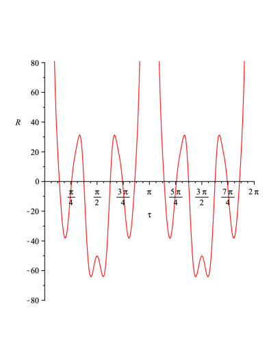
Figure 25: The evolution of the $R$ with respect of the cosmic time $\tau$ for Eq.(5.17)

In Fig.25 we plot the evolution of the $R$ with respect of the cosmic time $\tau$. In this example, we have shown that the Einstein equations admit the spike-like solution. We can show this solution describes the accelerated and decelerated expansion phases of the universe.

5.1.2 Example 2

The system (2.25)–(2.28) admits the following solution

$$H_{1} = \alpha\cos[(n-1)\tau]+\alpha(n-1)\cos[\tau],$$ (5.18)

$$H_{2} = \alpha\sin[(n-1)\tau]-\alpha(n-1)\sin[\tau],$$ (5.19)

$$H_{3} = \sin(\tau).$$ (5.20)

The corresponding EoS takes the form

$$\rho = \frac{D_{12}}{E_{12}},$$ (5.21)

$$p_{1} = -\frac{D_{13}}{E_{13}},$$ (5.22)

$$p_{2} = -\frac{D_{14}}{E_{14}},$$ (5.23)

$$p_{3} = -\frac{D_{15}}{E_{15}},$$ (5.24)

where

$$D_{12} = [\alpha\cos((n-1)\tau)+\alpha(n-1)\cos(\tau)][\alpha\sin((n-1)\tau)+[1-\alpha(n-1)]\sin(\tau)]+$$ (5.25)

$$[\alpha\sin((n-1)\tau)-\alpha(n-1)\sin(\tau)]\sin(\tau),$$

$$E_{12} = 1,$$ (5.26)

$$D_{13} = \alpha(n-1)[\cos((n-1)\tau)-\cos(\tau)]+\cos(\tau)+[\alpha\sin((n-1)\tau)-\alpha(n-1)\sin(\tau)]^{2}+$$ (5.27)

$$[\alpha\sin((n-1)\tau)+[1-\alpha(n-1)]\sin(\tau)]\sin(\tau),$$

$$E_{13} = 1,$$ (5.28)

$$D_{14} = -\alpha\sin((n-1)\tau)(n-1)-\alpha(n-1)\sin(\tau)+\cos(\tau)+[\alpha\cos((n-1)\tau)+\alpha(n-1)\cos(\tau)]^{2}+$$ (5.29)

$$\sin(\tau)^{2}+[\alpha\cos((n-1)\tau)+\alpha*(n-1)\cos(\tau)]\sin(\tau),$$

$$E_{14} = 1,$$ (5.30)

$$D_{15} = \alpha(n-1)[\cos((n-1)\tau)-\cos(\tau)-\sin((n-1)\tau)-\sin(\tau)]+$$ (5.31)

$$[\alpha\sin((n-1)\tau)-\alpha(n-1)\sin(\tau)]^{2}+[\alpha\cos((n-1)\tau)+\alpha(n-1)\cos(\tau)]^{2}+$$

$$[\alpha\cos((n-1)\tau)+\alpha(n-1)\cos(\tau)][\alpha\sin((n-1)\tau)-\alpha(n-1)\sin(\tau)],$$

$$E_{15} = 1.$$ (5.32)

The scalar curvature has the form

$$R = 2\alpha^{2}\cos((n-1)\tau)^{2}+4\alpha((1/2)\alpha\sin((n-1)\tau)+(1/2+(-(1/2)n+1/2)\alpha)\sin(\tau)+$$ (5.33)

$$+(n-1)(\alpha\cos(\tau)+1/2))\cos((n-1)\tau)+2\alpha^{2}\sin((n-1)\tau)^{2}+2\alpha((1+(2-2n)\alpha)\sin(\tau)+$$

$$+(\alpha\cos(\tau)-1)(n-1))\sin((n-1)\tau)+(2+2\alpha^{2}(n-1)^{2}+(2-2n)\alpha)\sin(\tau)^{2}-(2(n-1))\alpha*$$

$$*(1+(-1+\alpha(n-1))\cos(\tau))\sin(\tau)+(2(\alpha^{2}(n-1)^{2}\cos(\tau)+1+\alpha(-n+1)))\cos(\tau).$$

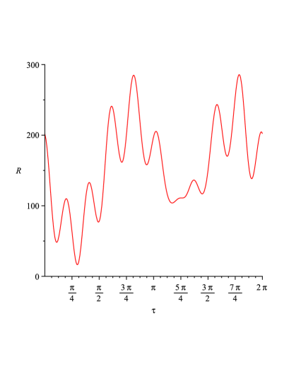
Figure 26: The evolution of the $R$ with respect of the cosmic time $\tau$ for Eq.(5.33)

In Fig.26 we plot the evolution of the $R$ with respect of the cosmic time $\tau$.

5.1.3 Example 3

Our next solution for the system (2.25)–(2.28) is given by

$$H_{1} = \alpha\cos[(n-1)\tau]-\alpha(n-1)\cos[\tau],$$ (5.34)

$$H_{2} = \alpha\sin[(n-1)\tau]-\alpha(n-1)\sin[\tau],$$ (5.35)

$$H_{3} = \sin(\tau).$$ (5.36)

In Fig.27 we plot this spiky type solution.

Figure 27: The evolution of the spiky type solution (5.34)-(5.36) with $n=10,\alpha=1$.

The corresponding EoS takes the form

$$\rho = \frac{D_{16}}{E_{16}},$$ (5.37)

$$p_{1} = -\frac{D_{17}}{E_{17}},$$ (5.38)

$$p_{2} = -\frac{D_{18}}{E_{18}},$$ (5.39)

$$p_{3} = -\frac{D_{19}}{E_{19}},$$ (5.40)

where

$$D_{16} = [\alpha\cos((n-1)\tau)-\alpha(n-1)\cos(\tau)][\alpha\sin((n-1)\tau)+[1-\alpha(n-1)]\sin(\tau)]+$$ (5.41)

$$[\alpha\sin((n-1)\tau)-\alpha(n-1)\sin(\tau)]\sin(\tau),$$

$$E_{16} = 1,$$ (5.42)

$$D_{17} = \alpha(n-1)[\cos((n-1)\tau)-\cos(\tau)]+\cos(\tau)+[\alpha\sin((n-1)\tau)-\alpha(n-1)\sin(\tau)]^{2}+$$ (5.43)

$$[\alpha\sin((n-1)\tau)+[1-\alpha(n-1)]\sin(\tau)]\sin(\tau),$$

$$E_{17} = 1,$$ (5.44)

$$D_{18} = -\alpha\sin((n-1)\tau)(n-1)+\alpha(n-1)\sin(\tau)+\cos(\tau)+[\alpha\cos((n-1)\tau)-\alpha(n-1)\cos(\tau)]^{2}+$$ (5.45)

$$\sin(\tau)^{2}+[\alpha\cos((n-1)\tau)-\alpha*(n-1)\cos(\tau)]\sin(\tau),$$

$$E_{18} = 1,$$ (5.46)

$$D_{19} = \alpha(n-1)[\cos((n-1)\tau)-\cos(\tau)-\sin((n-1)\tau)+\sin(\tau)]+$$ (5.47)

$$[\alpha\sin((n-1)\tau)-\alpha(n-1)\sin(\tau)]^{2}+[\alpha\cos((n-1)\tau)-\alpha(n-1)\cos(\tau)]^{2}+$$

$$[\alpha\cos((n-1)\tau)-\alpha(n-1)\cos(\tau)][\alpha\sin((n-1)\tau)-\alpha(n-1)\sin(\tau)],$$

$$E_{19} = 1.$$ (5.48)

The scalar curvature has the form

$$R = 2\alpha^{2}\cos((n-1)\tau)^{2}-(4(-(1/2)\alpha\sin((n-1)\tau)+(-1/2+((1/2)n-1/2)\alpha)\sin(\tau)+$$ (5.49)

$$+(n-1)(-1/2+\alpha\cos(\tau))))\alpha\cos((n-1)\tau)+2\alpha^{2}\sin((n-1)\tau)^{2}-$$

$$-(2((-1+(-2+2n)\alpha)\sin(\tau)+(\alpha\cos(\tau)+1)(n-1)))\alpha\sin((n-1)\tau)+$$

$$+(2+2\alpha^{2}(n-1)^{2}+(-2n+2)\alpha)\sin(\tau)^{2}+(2(n-1))(1+(-1+\alpha(n-1))*$$

$$*\cos(\tau))\alpha\sin(\tau)+2\cos(\tau)(\alpha^{2}(n-1)^{2}\cos(\tau)+1+(1-n)\alpha).$$

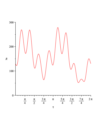
Figure 28: The evolution of the $R$ with respect of the cosmic time $\tau$ for Eq.(5.49)

In Fig.28 we plot the evolution of the $R$ with respect of the cosmic time $\tau$.

5.2 M$\ddot{o}$bius strip universe solutions

If we consider the model with the ”cosmological constant”, then the systems (2.21)–(2.24) and (2.25)–(2.28) take the form, respectively

$$\frac{\dot{A}\dot{B}}{AB}+\frac{\dot{B}\dot{C}}{BC}+\frac{\dot{C}\dot{A}}{CA}-\rho-\Lambda = 0,$$ (5.50)

$$\frac{\ddot{B}}{B}+\frac{\ddot{C}}{C}+\frac{\dot{B}\dot{C}}{BC}+p_{1}-\Lambda = 0,$$ (5.51)

$$\frac{\ddot{C}}{C}+\frac{\ddot{A}}{A}+\frac{\dot{C}\dot{A}}{CA}+p_{2}-\Lambda = 0,$$ (5.52)

$$\frac{\ddot{A}}{A}+\frac{\ddot{B}}{B}+\frac{\dot{A}\dot{B}}{AB}+p_{3}-\Lambda = 0$$ (5.53)

and

$$H_{1}H_{2}+H_{2}H_{3}+H_{1}H_{3}-\rho-\Lambda = 0,$$ (5.54)

$$\dot{H}_{2}+\dot{H}_{3}+H^{2}_{2}+H^{2}_{3}+H_{2}H_{3}+p_{1}-\Lambda = 0,$$ (5.55)

$$\dot{H}_{3}+\dot{H}_{1}+H^{2}_{3}+H^{2}_{1}+H_{3}H_{1}+p_{2}-\Lambda = 0,$$ (5.56)

$$\dot{H}_{1}+\dot{H}_{2}+H^{2}_{1}+H^{2}_{2}+H_{1}H_{2}+p_{3}-\Lambda = 0.$$ (5.57)

Now we want to present some solutions of these systems. Consider examples.

5.2.1 Example 1

One of the simplest solutions of (5.50)–(5.53) is given by

$$A = A_{0}+\left(1+\frac{1}{2}\Lambda\cos\frac{\tau}{2}\right)\cos\tau,$$ (5.58)

$$B = B_{0}+\left(1+\frac{1}{2}\Lambda\cos\frac{\tau}{2}\right)\sin\tau,$$ (5.59)

$$C = C_{0}+\frac{1}{2}\Lambda\sin\frac{\tau}{2}.$$ (5.60)

It is the parametric equation of the M$\ddot{o}$bius strip and, hence, such model we call the M$\ddot{o}$bius strip universe. Its plot was presented in Fig.29.

Figure 29: The plot of the M$\ddot{o}$bius strip universe for (5.58)–(5.60) with (3.16) and $\tau=0\rightarrow 2\pi$ and $\Lambda=[-1.1]$

The evolution of the volume of the M$\ddot{o}$bius strip universe for (5.58)–(5.60) with (3.16) reads as

$$V=0.5\Lambda\left(1+\frac{1}{2}\Lambda\cos\frac{\tau}{2}\right)^{2}\cos\tau\sin\tau\sin\frac{\tau}{2}.$$ (5.61)

The evolution of the volume with(3.16) and $\alpha=\Lambda=1$ presented in Fig.30.

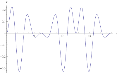
Figure 30: The evolution of the volume of the M$\ddot{o}$bius strip universe for (5.58)–(5.60) with (3.16) and $\alpha=\Lambda=1$.

The corresponding EoS takes the form

$$\rho = \frac{D_{20}}{E_{20}},$$ (5.62)

$$p_{1} = -\frac{D_{21}}{E_{21}},$$ (5.63)

$$p_{2} = -\frac{D_{22}}{E_{22}},$$ (5.64)

$$p_{3} = -\frac{D_{23}}{E_{23}},$$ (5.65)

where

$$D_{20} = [\frac{1}{4}\Lambda\sin(\frac{\tau}{2})\cos(\tau)+(1+\frac{1}{2}\Lambda\cos(\frac{\tau}{2}))\sin(\tau)][\frac{1}{4}\Lambda\sin(\frac{\tau}{2})\sin(\tau)-(1+\frac{1}{2}\Lambda\cos(\frac{\tau}{2})\cos(\tau)]\times$$ (5.66)

$$[C_{0}+\frac{1}{2}\Lambda\sin(\frac{\tau}{2})]+\frac{\Lambda}{4}[-\frac{1}{4}\Lambda\sin(\frac{\tau}{2})\sin(\tau)+(1+\frac{1}{2}\Lambda\cos(\frac{\tau}{2}))\cos(\tau)]\cos(\frac{\tau}{2})\times$$

$$[A_{0}+(1+\frac{1}{2})\Lambda\cos(\frac{\tau}{2})\cos(\tau)]+\frac{\Lambda}{4}[-\frac{1}{4}\Lambda\sin(\frac{\tau}{2})\cos(\tau)-(1+\frac{1}{2}\Lambda\cos(\frac{\tau}{2}))\sin(\tau)]\cos(\frac{\tau}{2})\times$$

$$[B_{0}+(1+\frac{1}{2})\Lambda\cos(\frac{\tau}{2}))\sin(\tau)]-\Lambda[A_{0}+(1+\frac{1}{2})\Lambda\cos(\frac{\tau}{2}))\cos(\tau)]\times$$

$$[B_{0}+(1+\frac{1}{2}\Lambda\cos(\frac{\tau}{2}))\sin(\tau)][C_{0}+\frac{1}{2}\Lambda\sin(\frac{\tau}{2})],$$

$$E_{20} = [A_{0}+(1+\frac{1}{2}\Lambda\cos(\frac{\tau}{2}))\cos(\tau)][B_{0}+(1+\frac{1}{2}\Lambda\cos(\frac{\tau}{2}))\sin(\tau)][C_{0}+\frac{1}{2}\Lambda\sin(\frac{\tau}{2})],$$ (5.67)

$$D_{21} = [C_{0}+\frac{1}{2}\Lambda\sin(\frac{\tau}{2})][-\frac{1}{8}\sin(\tau)\Lambda\cos(\frac{\tau}{2})-\frac{1}{2}\Lambda\sin(\frac{\tau}{2})\cos(\tau)-(1+\frac{1}{2}\Lambda\cos(\frac{\tau}{2}))\sin(\tau)]-$$ (5.68)

$$\frac{\Lambda}{8}[B_{0}+(1+\frac{1}{2}\Lambda\cos(\frac{\tau}{2}))\sin(\tau)]\sin(\frac{\tau}{2})+\frac{\Lambda}{4}[-\frac{1}{4}\Lambda\sin(\frac{\tau}{2})\sin(\tau)+(1+\frac{1}{2}\Lambda\cos(\frac{\tau}{2}))\times$$

$$\cos(\tau)]\cos(\frac{\tau}{2})-\Lambda[B_{0}+(1+\frac{1}{2}\Lambda\cos(\frac{\tau}{2}))\sin(\tau)][C_{0}+\frac{1}{2}\Lambda\sin(\frac{\tau}{2})],$$

$$E_{21} = [B_{0}+(1+\frac{1}{2}\Lambda\cos(\frac{\tau}{2}))\sin(\tau)][C_{0}+\frac{1}{2}\Lambda\sin(\frac{\tau}{2})],$$ (5.69)

$$D_{22} = -\frac{\Lambda}{8}[A_{0}+(1+\frac{1}{2}\cos(\frac{\tau}{2}))\cos(\tau)]\Lambda\sin(\frac{\tau}{2})+[C_{0}+\frac{1}{2}\Lambda\sin(\frac{\tau}{2})][-\frac{\Lambda}{8}\cos(\tau)\cos(\frac{\tau}{2})+$$ (5.70)

$$\frac{1}{2}\Lambda\sin(\frac{\tau}{2})\sin(\tau)-(1+\frac{1}{2}\Lambda\cos(\frac{\tau}{2}))\cos(\tau)]+\frac{1}{4}[-\frac{1}{4}\Lambda\sin(\frac{\tau}{2})\cos(\tau)-$$

$$(1+\frac{1}{2}\Lambda\cos(\frac{\tau}{2}))\sin(\tau)]\Lambda\cos(\frac{\tau}{2})-\Lambda[A_{0}+(1+\frac{1}{2}\Lambda\cos(\frac{\tau}{2}))\cos(\tau)][C_{0}+\frac{1}{2}\Lambda\sin(\frac{\tau}{2})],$$

$$E_{22} = [A_{0}+(1+\frac{1}{2}\Lambda\cos(\frac{\tau}{2}))\cos(\tau)][C_{0}+\frac{1}{2}\Lambda\sin(\frac{\tau}{2})],$$ (5.71)

$$D_{23} = [B_{0}+(1+\frac{1}{2}\Lambda\cos(\frac{\tau}{2}))\sin(\tau)][-\frac{\Lambda}{8}\cos(\tau)\cos(\frac{\tau}{2})+\frac{1}{2}\Lambda\sin(\frac{\tau}{2})\sin(\tau)-(1+\frac{1}{2}\Lambda\cos(\frac{\tau}{2}))\times$$ (5.72)

$$\cos(\tau)]+[A_{0}+(1+\frac{1}{2}\Lambda\cos(\frac{\tau}{2}))\cos(\tau)][-\frac{\Lambda}{8}\sin(\tau)\cos(\frac{\tau}{2})-\frac{1}{2}\Lambda\sin(\frac{\tau}{2})\cos(\tau)-$$

$$(1+\frac{1}{2}\Lambda\cos(\frac{\tau}{2}))\sin(\tau)]-[\frac{1}{4}\Lambda\sin(\frac{\tau}{2})\cos(\tau)+(1+\frac{1}{2}\Lambda\cos(\frac{\tau}{2}))\sin(\tau)]\times$$

$$[-\frac{1}{4}\Lambda\sin(\frac{\tau}{2})\sin(\tau)+(1+\frac{1}{2}\Lambda\cos(\frac{\tau}{2}))\cos(\tau)]-$$

$$\Lambda[A_{0}+(1+\frac{1}{2}\Lambda\cos(\frac{\tau}{2}))\cos(\tau)][B_{0}+(1+\frac{1}{2}\Lambda\cos(\frac{\tau}{2}))\sin(\tau)],$$

$$E_{23} = [B_{0}+(1+\frac{1}{2}\Lambda\cos(\frac{\tau}{2}))\sin(\tau)][A_{0}+(1+\frac{1}{2}\Lambda\cos(\frac{\tau}{2}))\cos(\tau)].$$ (5.73)

The scalar curvature has the form

$$R = ((-2\sin(\tau)^{2}\Lambda^{2}+2\cos(\tau)^{2}\Lambda^{2})\cos((1/2)\tau)^{3}+$$ (5.74)

$$+(-8\sin(\tau)^{2}\Lambda-17\cos(\tau)\sin(\tau)\sin((1/2)\tau)\Lambda^{2}+$$

$$+8\cos(\tau)^{2}\Lambda)\cos((1/2)\tau)^{2}+((6\sin(\tau)^{2}\Lambda^{2}-6\cos(\tau)^{2}\Lambda^{2})\sin((1/2)\tau)^{2}-$$

$$-60\cos(\tau)\sin(\tau)\sin((1/2)\tau)\Lambda+8\cos(\tau)^{2}-8\sin(\tau)^{2})\cos((1/2)\tau)+$$

$$+(\sin((1/2)\tau)^{2}\Lambda^{2}\cos(\tau)\sin(\tau)+(12\sin(\tau)^{2}\Lambda-12\cos(\tau)^{2}\Lambda)\sin((1/2)\tau)-$$

$$-52\cos(\tau)\sin(\tau))\sin((1/2)\tau))/(\sin(\tau)\cos(\tau)(2+\Lambda\cos((1/2)\tau))^{2}\sin((1/2)\tau)).$$

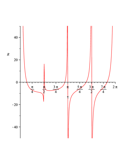
Figure 31: The evolution of the $R$ with respect of the cosmic time $\tau$ for Eq.(5.74)

In Fig.31 we plot the evolution of the $R$ with respect of the cosmic time $\tau$. In this subsubsection, we have shown that the Einstein equations have the M$\ddot{o}$bius strip universe solution. Again we can show that this solution describes the accelerated and decelerated expansion phases of the universe.

5.2.2 Example 2

For the system (5.54)–(5.57) the Mobious solution reads as

$$H_{1} = \left(1+\frac{1}{2}\Lambda\cos(\frac{\tau}{2})\right)\cos(\tau),$$ (5.75)

$$H_{2} = \left(1+\frac{1}{2}\Lambda\cos(\frac{\tau}{2})\right)\sin(\tau),$$ (5.76)

$$H_{3} = \frac{1}{2}\Lambda\sin(\frac{\tau}{2}).$$ (5.77)

The corresponding EoS takes the form

$$\rho = \frac{D_{24}}{E_{24}},$$ (5.78)

$$p_{1} = -\frac{D_{25}}{E_{25}},$$ (5.79)

$$p_{2} = -\frac{D_{26}}{E_{26}},$$ (5.80)

$$p_{3} = -\frac{D_{27}}{E_{27}},$$ (5.81)

where

$$D_{24} = [1+\frac{1}{2}\Lambda\cos(\frac{\tau}{2})]^{2}\cos(\tau)\sin(\tau)+\frac{\Lambda}{2}[1+\frac{\Lambda}{2}\cos(\frac{\tau}{2})][\sin(\tau)+\cos(\tau)]\sin(\frac{\tau}{2})-\Lambda,$$ (5.82)

$$E_{24} = 1,$$ (5.83)

$$D_{25} = -\frac{1}{4}\Lambda\sin(\frac{\tau}{2})\sin(\tau)+[1+\frac{1}{2}\Lambda\cos(\frac{\tau}{2})][\cos(\tau)+\frac{\Lambda}{2}\sin(\tau)\sin(\frac{\tau}{2})]+\frac{1}{4}\Lambda\cos(\frac{\tau}{2})+$$ (5.84)

$$[1+\frac{1}{2}\Lambda\cos(\frac{\tau}{2})]^{2}\sin^{2}(\tau)+\frac{\Lambda^{2}}{4}\sin^{2}(\frac{\tau}{2})-\Lambda,$$

$$E_{25} = 1,$$ (5.85)

$$D_{26} = -\frac{1}{4}\Lambda\sin(\frac{\tau}{2})\cos(\tau)-[1+\frac{1}{2}\Lambda\cos(\frac{\tau}{2})][\sin(\tau)+\frac{\Lambda}{2}\cos(\tau)\sin(\frac{\tau}{2})]+\frac{1}{4}\Lambda\cos(\frac{\tau}{2})+$$ (5.86)

$$[1+\frac{1}{2}\Lambda\cos(\frac{\tau}{2})]^{2}\cos^{2}(\tau)+\frac{\Lambda^{2}}{4}\sin^{2}(\frac{\tau}{2})-\Lambda,$$

$$E_{26} = 1,$$ (5.87)

$$D_{27} = [1+\frac{\Lambda}{2}\cos(\frac{\tau}{2})-\frac{\Lambda}{4}\sin(\frac{\tau}{2})][\cos(\tau)+\sin(\tau)]+$$ (5.88)

$$[1+\frac{\Lambda}{2}\cos(\frac{\tau}{2})]^{2}[1+\cos(\tau)\sin(\tau)]-\Lambda,$$

$$E_{27} = 1.$$ (5.89)

The scalar curvature has the form

$$R = (1/2)\Lambda^{2}(\cos^{2}(\tau)+\sin^{2}(\tau)+\cos(\tau)\sin(\tau))\cos^{2}((1/2)\tau)+$$ (5.90)

$$+(1/2((\cos(\tau)+\sin(\tau))\Lambda\sin((1/2)\tau)+4\cos^{2}(\tau)+(2+4\sin(\tau))\cos(\tau)+$$

$$+1-2\sin(\tau)+4\sin^{2}(\tau)))\Lambda\cos((1/2)\tau)+(1/2)\Lambda^{2}\sin^{2}((1/2)\tau)+$$

$$+(1/2(\cos(\tau)+\sin(\tau)))\Lambda\sin((1/2)\tau)+$$

$$+2\cos^{2}(\tau)+(1/2(4+4\sin(\tau)))\cos(\tau)-2\sin(\tau)+2\sin^{2}(\tau)$$

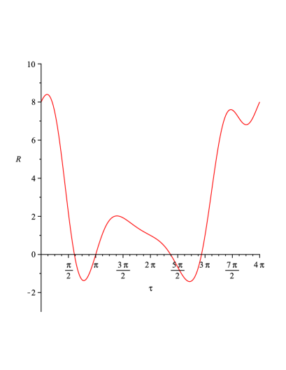
Figure 32: The evolution of the $R$ with respect of the cosmic time $\tau$ for Eq.(5.90)

In Fig.32 we plot the evolution of the $R$ with respect of the cosmic time $\tau$.

5.3 Other examples of M$\ddot{o}$bius strip like universes induced by Jacobian elliptic functions

5.3.1 Example 1

Now we want present some solutions in terms of the Jacobian elliptic functions. In fact, the system (5.50)–(5.53) has the following particular solution

$$A = A_{0}+\left(1+\frac{1}{2}\Lambda\mbox{cn}\frac{\tau}{2}\right)\mbox{cn}\tau,$$ (5.91)

$$B = B_{0}+\left(1+\frac{1}{2}\Lambda\mbox{cn}\frac{\tau}{2}\right)\mbox{sn}\tau,$$ (5.92)

$$C = C_{0}+\frac{1}{2}\Lambda\mbox{sn}\frac{\tau}{2}.$$ (5.93)

The corresponding EoS takes the form

$$\rho = \frac{D_{28}}{E_{28}},$$ (5.94)

$$p_{1} = -\frac{D_{29}}{E_{29}},$$ (5.95)

$$p_{2} = -\frac{D_{30}}{E_{30}},$$ (5.96)

$$p_{3} = -\frac{D_{31}}{E_{31}},$$ (5.97)

where

$$D_{28} = [\frac{1}{4}\Lambda\mbox{dn}\frac{\tau}{2}\ \mbox{sn}\frac{\tau}{2}\ \mbox{cn}\tau+(1+\frac{1}{2}\Lambda\mbox{cn}\frac{\tau}{2})\ \mbox{dn}\tau\ \mbox{sn}\tau][\frac{1}{4}\Lambda\mbox{dn}\frac{\tau}{2}\ \mbox{sn}\frac{\tau}{2}\ \mbox{sn}\tau-(1+\frac{1}{2}\Lambda\mbox{cn}\frac{\tau}{2})\ \mbox{cn}\tau\ \mbox{dn}\tau]\times$$ (5.98)

$$[C_{0}+\frac{1}{2}\Lambda\mbox{sn}\frac{\tau}{2}]+\frac{\Lambda}{4}[-\frac{1}{4}\Lambda\mbox{dn}\frac{\tau}{2}\ \mbox{sn}\frac{\tau}{2}\ \mbox{sn}\tau+(1+\frac{1}{2}\Lambda\mbox{cn}\frac{\tau}{2})\ \mbox{cn}\tau\ \mbox{dn}\tau]\mbox{cn}\frac{\tau}{2}\ \mbox{dn}\frac{\tau}{2}\times$$

$$[A_{0}+(1+\frac{1}{2}\Lambda\mbox{cn}\frac{\tau}{2})\mbox{cn}\tau]-\frac{1}{4}[\frac{1}{4}\Lambda\mbox{dn}\frac{\tau}{2}\ \mbox{sn}\frac{\tau}{2}\ \mbox{cn}\tau+(1+\frac{1}{2}\Lambda\mbox{cn}\frac{\tau}{2})\ \mbox{dn}\tau\ \mbox{sn}\tau]\Lambda\mbox{cn}\frac{\tau}{2}\ \mbox{dn}\frac{\tau}{2}\times$$

$$[B_{0}+(1+\frac{1}{2}\Lambda\mbox{cn}\frac{\tau}{2})\ \mbox{sn}\tau]-\Lambda[A_{0}+(1+\frac{1}{2}\Lambda\mbox{cn}\frac{\tau}{2})\ \mbox{cn}\tau][B_{0}+(1+\frac{1}{2}\Lambda\mbox{cn}\frac{\tau}{2})\ \mbox{sn}\tau]\times$$

$$[C_{0}+\frac{1}{2}\Lambda\mbox{sn}\frac{\tau}{2}],$$

$$E_{28} = [A_{0}+(1+\frac{1}{2}\Lambda\mbox{cn}\frac{\tau}{2})\ \mbox{cn}\tau][B_{0}+(1+\frac{1}{2}\Lambda\mbox{cn}\frac{\tau}{2})\ \mbox{sn}\tau][C_{0}+\frac{1}{2}\Lambda\mbox{sn}\frac{\tau}{2}],$$ (5.99)

$$D_{29} = [C_{0}+\frac{1}{2}\Lambda\mbox{sn}\frac{\tau}{2}][\frac{1}{8}\Lambda\mbox{cn}\frac{\tau}{2}\ \mbox{sn}^{2}\frac{\tau}{2}\ \mbox{sn}\tau-\frac{1}{8}\Lambda\mbox{dn}^{2}\frac{\tau}{2}\ \mbox{cn}\frac{\tau}{2}\ \mbox{sn}\tau-\frac{1}{2}\Lambda\mbox{dn}\frac{\tau}{2}\ \mbox{sn}\frac{\tau}{2}\ \mbox{cn}\tau\ \mbox{dn}\tau-$$ (5.100)

$$(1+\frac{1}{2}\Lambda\mbox{cn}\frac{\tau}{2})\ \mbox{dn}^{2}\tau\ \mbox{sn}\tau-[1+\frac{1}{2}\Lambda\mbox{cn}\frac{\tau}{2}]\ \mbox{cn}^{2}\tau\ \mbox{sn}\tau]+[B_{0}+(1+\frac{1}{2}\Lambda\mbox{cn}\frac{\tau}{2})\ \mbox{sn}\tau]\times$$

$$[-\frac{1}{8}\Lambda\mbox{dn}^{2}\frac{\tau}{2}\ \mbox{sn}\frac{\tau}{2}-\frac{1}{8}\Lambda\mbox{cn}^{2}\frac{\tau}{2}\mbox{sn}\frac{\tau}{2}]-\frac{\Lambda}{4}[\frac{1}{4}\Lambda\mbox{dn}\frac{\tau}{2}\ \mbox{sn}\frac{\tau}{2}\ \mbox{sn}\tau-(1+\frac{1}{2}\Lambda\mbox{cn}\frac{\tau}{2})\ \mbox{cn}\tau\ \mbox{dn}\tau]\times$$

$$\mbox{cn}\frac{\tau}{2}\ \mbox{dn}\frac{\tau}{2}-\Lambda[B_{0}+(1+\frac{1}{2}\Lambda\mbox{cn}\frac{\tau}{2})\ \mbox{sn}\tau][C_{0}+\frac{1}{2}\Lambda\mbox{sn}\frac{\tau}{2}],$$

$$E_{29} = [B_{0}+(1+\frac{1}{2}\Lambda\mbox{cn}\frac{\tau}{2})\ \mbox{sn}\tau][C_{0}+\frac{1}{2}\Lambda\mbox{sn}\frac{\tau}{2}],$$ (5.101)

$$D_{30} = -[A_{0}+(1+\frac{1}{2}\Lambda\ \mbox{cn}\frac{\tau}{2})\ \mbox{cn}\tau][\frac{1}{8}\Lambda\ \mbox{dn}^{2}\frac{\tau}{2}\ \mbox{sn}\frac{\tau}{2}+\frac{1}{8}\Lambda\ \mbox{cn}^{2}\frac{\tau}{2}\ \mbox{sn}\frac{\tau}{2}]+[C_{0}+\frac{1}{2}\Lambda\ \mbox{sn}\frac{\tau}{2}]\times$$ (5.102)

$$[\frac{1}{8}\Lambda\ \mbox{cn}\frac{\tau}{2}\ \mbox{sn}^{2}\frac{\tau}{2}\ \mbox{cn}\tau-\frac{1}{8}\Lambda\ \mbox{dn}^{2}\frac{\tau}{2}\ \mbox{cn}\frac{\tau}{2}\ \mbox{cn}\tau+\frac{1}{2}\Lambda\ \mbox{dn}\frac{\tau}{2}\ \mbox{sn}\frac{\tau}{2}\ \mbox{dn}\tau\ \mbox{sn}\tau+$$

$$(1+\frac{1}{2}\Lambda\ \mbox{cn}\frac{\tau}{2})(\mbox{cn}\tau\ \mbox{sn}^{2}\tau-\mbox{dn}^{2}\tau\ \mbox{cn}\tau)]-\frac{\Lambda}{4}[\frac{1}{4}\Lambda\ \mbox{dn}\frac{\tau}{2}\ \mbox{sn}\frac{\tau}{2}\ \mbox{cn}\tau+(1+\frac{1}{2}\Lambda\ \mbox{cn}\frac{\tau}{2})\times$$

$$\mbox{dn}\tau\ \mbox{sn}\tau]\ \mbox{cn}\frac{\tau}{2}\ \mbox{dn}\frac{\tau}{2}-\Lambda[A_{0}+(1+\frac{1}{2}\Lambda\ \mbox{cn}\frac{\tau}{2})\ \mbox{cn}\tau][C_{0}+\frac{1}{2}\Lambda\ \mbox{sn}\frac{\tau}{2}],$$

$$E_{30} = [A_{0}+(1+\frac{1}{2}\Lambda\ \mbox{cn}\frac{\tau}{2})\ \mbox{cn}\tau][C_{0}+\frac{1}{2}\Lambda\ \mbox{sn}\frac{\tau}{2}],$$ (5.103)

$$D_{31} = [B_{0}+(1+\frac{1}{2}\Lambda\ \mbox{cn}\frac{\tau}{2})\ \mbox{sn}\tau][\frac{1}{8}\Lambda\ \mbox{cn}\frac{\tau}{2}\ \mbox{sn}^{2}\frac{\tau}{2}\ \mbox{cn}\tau-\frac{1}{8}\Lambda\ \mbox{dn}^{2}\frac{\tau}{2}\ \mbox{cn}\frac{\tau}{2}\ \mbox{cn}\tau+$$ (5.104)

$$\frac{1}{2}\Lambda\ \mbox{dn}\frac{\tau}{2}\ \mbox{sn}\frac{\tau}{2}\ \mbox{dn}\tau\ \mbox{sn}\tau+(1+\frac{1}{2}\Lambda\ \mbox{cn}\frac{\tau}{2})(\mbox{sn}^{2}\tau-\ \mbox{dn}^{2}\tau)\ \mbox{cn}\tau]+[A_{0}+(1+\frac{1}{2}\Lambda\ \mbox{cn}\frac{\tau}{2})\ \mbox{cn}\tau]\times$$

$$[\frac{1}{8}\Lambda\ \mbox{cn}\frac{\tau}{2}\ \mbox{sn}\tau(\mbox{sn}^{2}\frac{\tau}{2}-\mbox{dn}^{2}\tau)-\frac{1}{2}\Lambda\ \mbox{dn}\frac{\tau}{2}\ \mbox{sn}\frac{\tau}{2}\ \mbox{cn}\tau\ \mbox{dn}\tau-(1+\frac{1}{2}\Lambda\ \mbox{cn}\frac{\tau}{2})\ \mbox{dn}^{2}\tau\ \mbox{sn}\tau-$$

$$(1+\frac{1}{2}\Lambda\ \mbox{cn}\frac{\tau}{2})\ \mbox{cn}^{2}\tau\ \mbox{sn}\tau]+[\frac{1}{4}\Lambda\ \mbox{dn}\frac{\tau}{2}\ \mbox{sn}\frac{\tau}{2}\ \mbox{cn}\tau+(1+\frac{1}{2}\Lambda\ \mbox{cn}\frac{\tau}{2})\ \mbox{dn}\tau\ \mbox{sn}\tau]\times$$

$$[\frac{1}{4}\Lambda\ \mbox{dn}\frac{\tau}{2}\ \mbox{sn}\frac{\tau}{2}\ \mbox{sn}\tau-(1+\frac{1}{2}\Lambda\ \mbox{cn}\frac{\tau}{2})\ \mbox{cn}\tau\ \mbox{dn}\tau]-\Lambda[A_{0}+(1+\frac{1}{2}\Lambda\ \mbox{cn}\frac{\tau}{2})\ \mbox{cn}\tau]\times$$

$$[B_{0}+(1+\frac{1}{2}\Lambda\ \mbox{cn}\frac{\tau}{2})\ \mbox{sn}\tau],$$

$$E_{31} = [B_{0}+(1+\frac{1}{2}\Lambda\ \mbox{cn}\frac{\tau}{2})\ \mbox{sn}\tau][A_{0}+(1+\frac{1}{2}\Lambda\ \mbox{cn}\frac{\tau}{2})\ \mbox{cn}\tau].$$ (5.105)

The evolution of the volume of the universe for (3.16) reads as ($A_{0}=B_{0}=C_{0}=0$)

$$V=\frac{1}{2}\Lambda\left(1+\frac{1}{2}\Lambda\mbox{cn}\frac{\tau}{2}\right)^{2}\mbox{cn}\tau\ \mbox{sn}\tau\ \mbox{sn}\frac{\tau}{2}.$$ (5.106)

The evolution of the volume with (3.16) and $\Lambda=1$ presented in Fig.33.

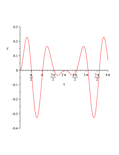
Figure 33: The evolution of the volume of the trefoil knot universe with respect to the cosmic time $\tau$ for Eq.(5.106)

The scalar curvature has the form

$$R = (2\Lambda(2k^{2}\mbox{cn}((1/2)\tau,k)+\Lambda k^{2}\mbox{cn}^{2}((1/2)\tau,k)+$$ (5.107)

$$+(1/2)\Lambda\mbox{dn}^{2}((1/2)\tau,k))\mbox{cn}(\tau,k)\mbox{sn}(\tau,k)\mbox{sn}((1/2)\tau,k)^{3}-$$

$$-6\Lambda\mbox{dn}(\tau,k)\mbox{dn}((1/2)\tau,k)(\mbox{cn}(\tau,k)-\mbox{sn}(\tau,k))(\mbox{cn}(\tau,k)+$$

$$+\mbox{sn}(\tau,k))(2+\Lambda\mbox{cn}((1/2)\tau,k))\mbox{sn}^{2}((1/2)\tau,k)-$$

$$-(4(2+\Lambda\mbox{cn}((1/2)\tau,k)))((1/4)\mbox{cn}^{3}((1/2)\tau,k)k^{2}\Lambda+$$

$$+(1/2)\mbox{cn}^{2}((1/2)\tau,k)k^{2}+\Lambda(3\mbox{dn}^{2}(\tau,k)+\mbox{cn}^{2}(\tau,k)k^{2}+(5/4)\mbox{dn}^{2}((1/2)\tau,k)-$$

$$-\mbox{sn}^{2}(\tau,k)k^{2})\mbox{cn}((1/2)\tau,k)+6\mbox{dn}^{2}(\tau,k)+(1/2)\mbox{dn}^{2}((1/2)\tau,k)-$$

$$-2\mbox{sn}^{2}(\tau,k)k^{2}+2\mbox{cn}^{2}(\tau,k)k^{2})\mbox{cn}(\tau,k)\mbox{sn}(\tau,k)\mbox{sn}((1/2)\tau,k)+$$

$$+2\mbox{cn}((1/2)\tau,k)\mbox{dn}((1/2)\tau,k)\mbox{dn}(\tau,k)(\mbox{cn}(\tau,k)-\mbox{sn}(\tau,k))(\mbox{cn}(\tau,k)+$$

$$+\mbox{sn}(\tau,k))(2+\Lambda\mbox{cn}((1/2)\tau,k))^{2})/(\mbox{cn}(\tau,k)\mbox{sn}(\tau,k)*$$

$$*(2+\Lambda\mbox{cn}^{2}((1/2)\tau,k))\mbox{sn}((1/2)\tau,k)).$$

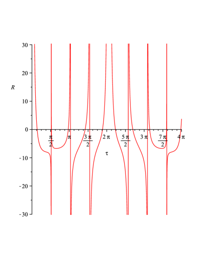
Figure 34: The evolution of the $R$ with respect of the cosmic time $\tau$ for Eq.(5.107)

In Fig.34 we plot the evolution of the $R$ with respect of the cosmic time $\tau$.

5.3.2 Example 2

Similarly, we can show that the system (5.54)–(5.57) has the following solution

$$H_{1} = \left(1+\frac{1}{2}\Lambda\mbox{cn}\frac{\tau}{2}\right)\mbox{cn}\tau,$$ (5.108)

$$H_{2} = \left(1+\frac{1}{2}\Lambda\mbox{cn}\frac{\tau}{2}\right)\mbox{sn}\tau,$$ (5.109)

$$H_{3} = \frac{1}{2}\Lambda\mbox{sn}\frac{\tau}{2}.$$ (5.110)

The corresponding EoS takes the form

$$\rho = \frac{D_{32}}{E_{32}},$$ (5.111)

$$p_{1} = -\frac{D_{33}}{E_{33}},$$ (5.112)

$$p_{2} = -\frac{D_{34}}{E_{34}},$$ (5.113)

$$p_{3} = -\frac{D_{35}}{E_{35}},$$ (5.114)

where

$$D_{32} = [1+\frac{1}{2}\ \Lambda\ \mbox{cn}\frac{\tau}{2}]^{2}\ \mbox{cn}\tau\ \mbox{sn}\tau+\frac{\Lambda}{2}\ [1+\frac{1}{2}\Lambda\ \mbox{cn}\frac{\tau}{2}][\mbox{sn}\tau+\mbox{cn}\tau]\ \mbox{sn}\frac{\tau}{2}-\Lambda,$$ (5.115)

$$E_{32} = 1,$$ (5.116)

$$D_{33} = \frac{1}{4}\Lambda\mbox{dn}\frac{\tau}{2}\ \mbox{sn}\frac{\tau}{2}[1-\mbox{sn}\tau]+[1+\frac{1}{2}\Lambda\ \mbox{cn}\frac{\tau}{2}][\mbox{cn}\tau\ \mbox{dn}\tau+\frac{\Lambda}{2}\ \mbox{sn}\tau\ \mbox{sn}\frac{\tau}{2}]+[1+\frac{1}{2}\Lambda\mbox{cn}\frac{\tau}{2}]^{2}\ \mbox{sn}^{2}\tau+$$ (5.117)

$$\frac{1}{4}\Lambda^{2}\mbox{sn}^{2}\frac{\tau}{2}-\Lambda,$$

$$E_{33} = 1,$$ (5.118)

$$D_{34} = -\frac{1}{4}\Lambda\ \mbox{dn}\frac{\tau}{2}\ \mbox{sn}\frac{\tau}{2}\ \mbox{cn}\tau-(1+\frac{1}{2}\Lambda\ \mbox{cn}\frac{\tau}{2})[\mbox{dn}\tau\ \mbox{sn}\tau+\frac{\Lambda}{2}\ \mbox{cn}\tau\ \mbox{sn}\frac{\tau}{2}]+\frac{1}{4}\Lambda\ \mbox{cn}\frac{\tau}{2}\ \mbox{dn}\frac{\tau}{2}+$$ (5.119)

$$[1+\frac{1}{2}\Lambda\ \mbox{cn}\frac{\tau}{2}]^{2}\ \mbox{cn}^{2}\tau+\frac{1}{4}\ \Lambda^{2}\ \mbox{sn}^{2}\frac{\tau}{2}-\Lambda,$$

$$E_{34} = 1,$$ (5.120)

$$D_{35} = -\frac{1}{4}\Lambda\ \mbox{dn}\frac{\tau}{2}\ \mbox{sn}\frac{\tau}{2}[\mbox{cn}\tau+\mbox{sn}\tau]+[1+\frac{1}{2}\Lambda\ \mbox{cn}\frac{\tau}{2}][\mbox{cn}\tau-\mbox{sn}\tau]\mbox{dn}\tau+$$ (5.121)

$$[1+\frac{1}{2}\ \Lambda\ \mbox{cn}\frac{\tau}{2}]^{2}[\mbox{sn}^{2}\tau+\mbox{cn}^{2}\tau+\mbox{cn}\tau\ \mbox{sn}\tau]-\Lambda,$$

$$E_{35} = 1.$$ (5.122)

The scalar curvature has the form

$$R = (1/2)\Lambda^{2}(\mbox{cn}^{2}(\tau,k)+\mbox{sn}^{2}(\tau,k)+\mbox{cn}(\tau,k)\mbox{sn}(\tau,k))\mbox{cn}^{2}((1/2)\tau,k)+$$ (5.123)

$$+(1/2(\Lambda(\mbox{sn}(\tau,k)+\mbox{cn}(\tau,k))\mbox{sn}((1/2)\tau,k)+\mbox{dn}((1/2)\tau,k)+4\mbox{cn}^{2}(\tau,k)+$$

$$+(4\mbox{sn}(\tau,k)+2\mbox{dn}(\tau,k))\mbox{cn}(\tau,k)+4\mbox{sn}^{2}(\tau,k)-$$

$$-2\mbox{dn}(\tau,k)\mbox{sn}(\tau,k)))\Lambda\mbox{cn}((1/2)\tau,k)+(1/2)\Lambda^{2}\mbox{sn}^{2}((1/2)\tau,k)-$$

$$-(1/2)\Lambda(\mbox{dn}((1/2)\tau,k)-2)(\mbox{sn}(\tau,k)+$$

$$+\mbox{cn}(\tau,k))\mbox{sn}((1/2)\tau,k)+2\mbox{cn}^{2}(\tau,k)+(1/2(4\mbox{dn}(\tau,k)+$$

$$+4\mbox{sn}(\tau,k)))\mbox{cn}(\tau,k)-2\mbox{sn}(\tau,k)(-\mbox{sn}(\tau,k)+\mbox{dn}(\tau,k)).$$

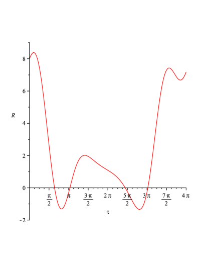
Figure 35: The evolution of the $R$ with respect of the cosmic time $\tau$ for Eq.(5.124)

In Fig.35 we plot the evolution of the $R$ with respect of the cosmic time $\tau$.

5.4 Integrable models

The system (2.21)-(2.24) contents 4 equations for 7 unknown functions. This means we can add 3 new additional equations. It gives us in particular to construct integrable Bianchi models. In this subsection we present two examples of such integrable models.

5.4.1 Euler top equation

Let us we assume that $A=A_{1},B=A_{2},C=A_{3}$ obey the Euler top equation. The simple Euler top equation reads as

$$\dot{A}_{1} = A_{2}A_{3},$$ (5.124)

$$\dot{A}_{2} = A_{3}A_{1},$$ (5.125)

$$\dot{A}_{3} = A_{1}A_{2}.$$ (5.126)

The system of equations (2.21)-(2.24) and (5.124)-(5.126) we call the Bianchi I-Euler model which is integrable.

5.4.2 Heisenberg ferromagnet equation

Our second example is the Heisenberg ferromagnet equation (HFE). Here we assume that the variables $A=S_{1},B=S_{2},C=S_{3}$ satisfy the equation $iS_{t}+\frac{1}{\omega}[S,W]=0,\quad iW_{x}+\omega[S,W]=0,$ where $S=S_{i}\sigma_{i}$, $W=W_{i}\sigma_{i}$ and $\sigma_{i}$ are Pauli’s matrices. It the principal chiral type equation with the $U=-i\lambda S,\quad V=-\frac{i\lambda}{\omega(\lambda+\omega)}W.$. Note this principal chiral type equation is the particular case of the following (2+1)-dimensional M-XCIX equation [47] (see also [48])

$$iS_{t}+0.5([S,S_{y}]+uS)_{x}+\frac{1}{\omega}[S,W] = 0,$$ (5.127)

$$u_{x}-0.5S\cdot[S_{x},S_{y}] = 0,$$ (5.128)

$$iW_{x}+\omega[S,W] = 0$$ (5.129)

or (that equivalent)

$$iS_{t}+0.5[S,S_{xy}]+uS_{x}+\frac{1}{\omega}[S,W] = 0,$$ (5.130)

$$u_{x}-0.5S\cdot[S_{x},S_{y}] = 0,$$ (5.131)

$$iW_{x}+\omega[S,W] = 0.$$ (5.132)

This M-XCIX equation is integrable by the following Lax representation [47]

$$\Phi_{x} = U\Phi,$$ (5.133)

$$\Phi_{t} = 2\lambda\Phi_{y}+V\Phi,$$ (5.134)

with ($S^{2}=I$)

$$U = -i\lambda S,$$ (5.135)

$$V = \lambda V_{1}+\frac{i}{\lambda+\omega}W-\frac{i}{\omega}W$$ (5.136)

and

$$S = \begin{pmatrix}S_{3}&S^{-}\\ S^{+}&-S_{3}\end{pmatrix},$$ (5.137)

$$V_{1} = 0.25([S,S_{y}]+uS),$$ (5.138)

$$W = \begin{pmatrix}W_{3}&W^{-}\\ W^{+}&-W_{3}\end{pmatrix}.$$ (5.139)

6 Conclusion

In the present paper, we have constructed several concrete models describing the trefoil and figure-eight knot universes from Bianchi-type I cosmology and examined the cosmological features and properties in detail.

To realize the cyclic universes, it is necessary to a non-canonical scalar field with non well-defined vacuum in the context of the quantum field theory or extend gravity, e.g., with adding higher order derivative terms and $f(R)$ gravity [25]. Indeed, however, these modified gravity theories have to satisfy the tests on the solar system scale as well as cosmological constraints so that those can be alternative gravitational theories to general relativity. The significant cosmological consequence of our approach is that we have shown the possibility to obtain the knot universes related to the cyclic universes from Bianchi-type I spacetime within general relativity.

Furthermore, recently it has been pointed out that the asymmetry of the EoS for the universe can lead to cosmological hysteresis [26]. On the other hand, Bianchi-type I spacetime describes the spatially anisotropic cosmology and hence the EoS for the universe has the asymmetry in the oscillating process through the expanding and contracting behaviors. Accordingly, it is considered that in the constructed models of the knot universes cosmological hysteresis could occur. The observation of this phenomenon in our models is one of our future works on the knot universes.

Finally, it should be remarked that by summarizing the results of our previous [30] and this works, the knot universes describing the cyclic universes can be realized from the homogeneous and isotropic FLRW spacetime as well as the homogeneous and anisotropic Bianchi-type I cosmology. In these series of works, the formulations of model construction method of the knot universes have been established. Thus, it can be expected that the presented formalism is useful to realize the universes with other features from both the isotropic and anisotropic spacetimes.

Finally we would like to note that all solutions presented above describe the accelerated and decelerated expansion phases of the universe.

References

- [1] D. N. Spergel et al. [WMAP Collaboration], Astrophys. J. Suppl. 148, 175 (2003) [arXiv:astro-ph/0302209]; Astrophys. J. Suppl. 170, 377 (2007) [arXiv:astro-ph/0603449]; E. Komatsu et al. [WMAP Collaboration], Astrophys. J. Suppl. 180, 330 (2009) [arXiv:0803.0547 [astro-ph]]; Astrophys. J. Suppl. 192, 18 (2011) [arXiv:1001.4538 [astro-ph.CO]].
- [2] S. Perlmutter et al. [SNCP Collaboration], Astrophys. J. 517, 565 (1999) [arXiv:astro-ph/9812133]; A. G. Riess et al. [Supernova Search Team Collaboration], Astron. J. 116, 1009 (1998) [arXiv:astro-ph/9805201].
- [3] M. Tegmark et al. [SDSS Collaboration], Phys. Rev. D 69, 103501 (2004) [arXiv:astro-ph/0310723]; U. Seljak et al. [SDSS Collaboration], Phys. Rev. D 71, 103515 (2005) [arXiv:astro-ph/0407372].
- [4] D. J. Eisenstein et al. [SDSS Collaboration], Astrophys. J. 633, 560 (2005) [arXiv:astro-ph/0501171].
- [5] B. Jain and A. Taylor, Phys. Rev. Lett. 91, 141302 (2003) [arXiv:astro-ph/0306046].
- [6] E. J. Copeland, M. Sami and S. Tsujikawa, Int. J. Mod. Phys. D 15, 1753 (2006) [arXiv:hep-th/0603057].
- [7] R. Durrer and R. Maartens, Gen. Rel. Grav. 40, 301 (2008) [arXiv:0711.0077 [astro-ph]]; arXiv:0811.4132 [astro-ph].
- [8] Y. F. Cai, E. N. Saridakis, M. R. Setare and J. Q. Xia, Phys. Rept. 493, 1 (2010) [arXiv:0909.2776 [hep-th]].
- [9] S. Tsujikawa, arXiv:1004.1493 [astro-ph.CO].
- [10] L. Amendola and S. Tsujikawa, Dark Energy (Cambridge University press, 2010).
- [11] M. Li, X. D. Li, S. Wang and Y. Wang, Commun. Theor. Phys. 56, 525 (2011) [arXiv:1103.5870 [astro-ph.CO]].
- [12] S. Nojiri and S. D. Odintsov, Phys. Rept. 505, 59 (2011) [arXiv:1011.0544 [gr-qc]]; eConf C0602061, 06 (2006) [Int. J. Geom. Meth. Mod. Phys. 4, 115 (2007)] [arXiv:hep-th/0601213].
- [13] T. P. Sotiriou and V. Faraoni, Rev. Mod. Phys. 82, 451 (2010) [arXiv:0805.1726 [gr-qc]].
- [14] S. Capozziello and V. Faraoni, Beyond Einstein Gravity (Springer, 2010).
- [15] S. Capozziello and M. De Laurentis, Phys. Rept. 509, 167 (2011) [arXiv:1108.6266 [gr-qc]].
- [16] A. De Felice and S. Tsujikawa, Living Rev. Rel. 13, 3 (2010) [arXiv:1002.4928 [gr-qc]].
- [17] T. Clifton, P. G. Ferreira, A. Padilla and C. Skordis, arXiv:1106.2476 [astro-ph.CO].
- [18] R. R. Caldwell, M. Kamionkowski and N. N. Weinberg, Phys. Rev. Lett. 91, 071301 (2003) [arXiv:astro-ph/0302506]; B. McInnes, JHEP 0208 (2002) 029 [arXiv:hep-th/0112066]; S. Nojiri and S. D. Odintsov, Phys. Lett. B 562, 147 (2003) [arXiv:hep-th/0303117]; Phys. Lett. B 571, 1 (2003) [arXiv:hep-th/0306212]; V. Faraoni, Int. J. Mod. Phys. D 11, 471 (2002) [arXiv:astro-ph/0110067]; P. F. Gonzalez-Diaz, Phys. Lett. B 586, 1 (2004) [arXiv:astro-ph/0312579]; E. Elizalde, S. Nojiri and S. D. Odintsov, Phys. Rev. D 70, 043539 (2004) [arXiv:hep-th/0405034]; P. Singh, M. Sami and N. Dadhich, Phys. Rev. D 68, 023522 (2003) [arXiv:hep-th/0305110]; C. Csaki, N. Kaloper and J. Terning, Annals Phys. 317, 410 (2005) [arXiv:astro-ph/0409596]; P. X. Wu and H. W. Yu, Nucl. Phys. B 727, 355 (2005) [arXiv:astro-ph/0407424]; S. Nesseris and L. Perivolaropoulos, Phys. Rev. D 70, 123529 (2004) [arXiv:astro-ph/0410309]; M. Sami and A. Toporensky, Mod. Phys. Lett. A 19, 1509 (2004) [arXiv:gr-qc/0312009]; H. Stefancic, Phys. Lett. B 586, 5 (2004) [arXiv:astro-ph/0310904]; L. P. Chimento and R. Lazkoz, Phys. Rev. Lett. 91, 211301 (2003) [arXiv:gr-qc/0307111]; J. G. Hao and X. Z. Li, Phys. Lett. B 606, 7 (2005) [arXiv:astro-ph/0404154]; E. Elizalde, S. Nojiri, S. D. Odintsov and P. Wang, Phys. Rev. D 71, 103504 (2005) [arXiv:hep-th/0502082]; M. P. Dabrowski and T. Stachowiak, Annals Phys. 321, 771 (2006) [arXiv:hep-th/0411199]; F. S. N. Lobo, Phys. Rev. D 71, 084011 (2005) [arXiv:gr-qc/0502099]; R. G. Cai, H. S. Zhang and A. Wang, Commun. Theor. Phys. 44, 948 (2005) [arXiv:hep-th/0505186]; I. Y. Aref’eva, A. S. Koshelev and S. Y. Vernov, Phys. Rev. D 72, 064017 (2005) [arXiv:astro-ph/0507067]; H. Q. Lu, Z. G. Huang and W. Fang, arXiv:hep-th/0504038; W. Godlowski and M. Szydlowski, Phys. Lett. B 623, 10 (2005) [arXiv:astro-ph/0507322]; J. Sola and H. Stefancic, Phys. Lett. B 624, 147 (2005) [arXiv:astro-ph/0505133]; B. Guberina, R. Horvat and H. Nikolic, Phys. Rev. D 72, 125011 (2005) [arXiv:astro-ph/0507666].
- [19] Y. Shtanov and V. Sahni, Class. Quant. Grav. 19, L101 (2002) [arXiv:gr-qc/0204040].
- [20] J. D. Barrow, Class. Quant. Grav. 21, L79 (2004) [arXiv:gr-qc/0403084].
- [21] S. Nojiri and S. D. Odintsov, Phys. Lett. B 595, 1 (2004) [arXiv:hep-th/0405078]; Phys. Rev. D 70, 103522 (2004) [arXiv:hep-th/0408170]; Phys. Rev. D 72, 023003 (2005) [arXiv:hep-th/0505215]; S. Cotsakis and I. Klaoudatou, J. Geom. Phys. 55, 306 (2005) [arXiv:gr-qc/0409022]; M. P. Dabrowski, Phys. Rev. D 71, 103505 (2005) [arXiv:gr-qc/0410033]; L. Fernandez-Jambrina and R. Lazkoz, Phys. Rev. D 70, 121503 (2004) [arXiv:gr-qc/0410124]; Phys. Lett. B 670, 254 (2009) [arXiv:0805.2284 [gr-qc]]; J. D. Barrow and C. G. Tsagas, Class. Quant. Grav. 22, 1563 (2005) [arXiv:gr-qc/0411045]; H. Stefancic, Phys. Rev. D 71, 084024 (2005) [arXiv:astro-ph/0411630]; C. Cattoen and M. Visser, Class. Quant. Grav. 22, 4913 (2005) [arXiv:gr-qc/0508045]; P. Tretyakov, A. Toporensky, Y. Shtanov and V. Sahni, Class. Quant. Grav. 23, 3259 (2006) [arXiv:gr-qc/0510104]; A. Balcerzak and M. P. Dabrowski, Phys. Rev. D 73, 101301 (2006) [arXiv:hep-th/0604034]; M. Sami, P. Singh and S. Tsujikawa, Phys. Rev. D 74, 043514 (2006) [arXiv:gr-qc/0605113]; M. Bouhmadi-Lopez, P. F. Gonzalez-Diaz and P. Martin-Moruno, Phys. Lett. B 659, 1 (2008) [arXiv:gr-qc/0612135]; A. V. Yurov, A. V. Astashenok and P. F. Gonzalez-Diaz, Grav. Cosmol. 14, 205 (2008) [arXiv:0705.4108 [astro-ph]]; T. Koivisto, Phys. Rev. D 77, 123513 (2008) [arXiv:0803.3399 [gr-qc]]; J. D. Barrow and S. Z. W. Lip, Phys. Rev. D 80, 043518 (2009) [arXiv:0901.1626 [gr-qc]]; M. Bouhmadi-Lopez, Y. Tavakoli and P. V. Moniz, JCAP 1004, 016 (2010) [arXiv:0911.1428 [gr-qc]].
- [22] S. Nojiri, S. D. Odintsov and S. Tsujikawa, Phys. Rev. D 71 (2005) 063004 [arXiv:hep-th/0501025].
- [23] S. Nojiri and S. D. Odintsov, Phys. Rev. D 78, 046006 (2008) [arXiv:0804.3519 [hep-th]]; K. Bamba, S. Nojiri and S. D. Odintsov, JCAP 0810 (2008) 045 [arXiv:0807.2575 [hep-th]]; K. Bamba, S. D. Odintsov, L. Sebastiani and S. Zerbini, Eur. Phys. J. C 67 (2010) 295 [arXiv:0911.4390 [hep-th]].
- [24] P. J. Steinhardt and N. Turok, Phys. Rev. D 65, 126003 (2002) [arXiv:hep-th/0111098]; arXiv:hep-th/0111030; J. Khoury, B. A. Ovrut, P. J. Steinhardt and N. Turok, Phys. Rev. D 66, 046005 (2002) [arXiv:hep-th/0109050]; P. J. Steinhardt and N. Turok, Nucl. Phys. Proc. Suppl. 124, 38 (2003) [arXiv:astro-ph/0204479]; Science 296, 1436 (2002); J. Khoury, P. J. Steinhardt and N. Turok, Phys. Rev. Lett. 92, 031302 (2004) [arXiv:hep-th/0307132]; P. J. Steinhardt and N. Turok, Science 312, 1180 (2006) [astro-ph/0605173]. K. Saaidi, H. Sheikhahmadi and A. H. Mohammadi, Astrophys. Space Sci. 338, 355 (2012) [arXiv:1201.0275 [gr-qc]]; S. Nojiri, S. D. Odintsov and D. Saez-Gomez, arXiv:1108.0767 [hep-th].
- [25] Y. F. Cai and E. N. Saridakis, J. Cosmol. 17, 7238 (2011) [arXiv:1108.6052 [gr-qc]].
- [26] V. Sahni and A. Toporensky, arXiv:1203.0395 [gr-qc].
- [27] D. Y. Chung, arXiv:physics/0105064.
- [28] J. Khoury, B. A. Ovrut, P. J. Steinhardt and N. Turok, Phys. Rev. D 64, 123522 (2001) [arXiv:hep-th/0103239]; arXiv:hep-th/0105212; R. Y. Donagi, J. Khoury, B. A. Ovrut, P. J. Steinhardt and N. Turok, JHEP 0111, 041 (2001) [arXiv:hep-th/0105199]; J. Khoury, B. A. Ovrut, P. J. Steinhardt and N. Turok, Phys. Rev. D 66, 046005 (2002) [arXiv:hep-th/0109050].
- [29] D. N. Page, Class. Quant. Grav. 1, 417 (1984). P. Peter and N. Pinto-Neto, Phys. Rev. D 65, 023513 (2001) [arXiv:gr-qc/0109038]; 66, 063509 (2002) [arXiv:hep-th/0203013]; Y. Shtanov and V. Sahni, Phys. Lett. B 557, 1 (2003) [arXiv:gr-qc/0208047]; T. Biswas, A. Mazumdar and W. Siegel, JCAP 0603, 009 (2006) [arXiv:hep-th/0508194]; Y. F. Cai, T. Qiu, Y. S. Piao, M. Li and X. Zhang, JHEP 0710, 071 (2007) [arXiv:0704.1090 [gr-qc]]; P. Creminelli and L. Senatore, JCAP 0711, 010 (2007) [arXiv:hep-th/0702165]; M. Novello and S. E. P. Bergliaffa, Phys. Rept. 463, 127 (2008) [arXiv:0802.1634 [astro-ph]]; Y. S. Piao, Phys. Lett. B 677, 1 (2009) [arXiv:0901.2644 [gr-qc]]; J. Zhang, Z. G. Liu and Y. S. Piao, Phys. Rev. D 82, 123505 (2010) [arXiv:1007.2498 [hep-th]]; Y. S. Piao, Phys. Lett. B 691, 225 (2010) [arXiv:1001.0631 [hep-th]]; Z. G. Liu and Y. S. Piao, arXiv:1201.1371 [gr-qc].
-
[30]
R. Myrzakulov,
arXiv:1008.4486; arXiv:1205.5266; arXiv:1207.1039;
R. Myrzakulov et al., arXiv:1102.4456;
R. Myrzakulov et al., arXiv:1201.4360;
R. Myrzakulov, arXiv:1204.1093. - [31] G. W. Gibbons and M. Vyska, Class. Quant. Grav. 29, 065016 (2012) [arXiv:1110.6508 [gr-qc]]; I. Bochicchio, S. Capozziello and E. Laserra, Int. J. Geom. Meth. Mod. Phys. 8, 1653 (2011) [arXiv:1111.0819 [gr-qc]]; B. G. Dimitrov, J. Math. Phys. 44, 2542 (2003) [arXiv:hep-th/0107231].
- [32] J. D’Ambroise, arXiv:0908.2481 [gr-qc].
- [33] S. Nojiri and S. D. Odintsov, Phys. Rev. D 72 (2005) 023003 [arXiv:hep-th/0505215].
- [34] H. Stefancic, Phys. Rev. D 71 (2005) 084024 [arXiv:astro-ph/0411630].
- [35] K. Bamba, K. Yesmakhanova, K. Yerzhanov and R. Myrzakulov, arXiv:1203.3401 [gr-qc].
- [36] A. Y. Kamenshchik, U. Moschella and V. Pasquier, Phys. Lett. B 511 (2001) 265 [arXiv:gr-qc/0103004].
- [37] M. C. Bento, O. Bertolami and A. A. Sen, Phys. Rev. D 66 (2002) 043507 [arXiv:gr-qc/0202064].
- [38] H. B. Benaoum, arXiv:hep-th/0205140.
-
[39]
K. Bamba, U. Debnath, K. Yesmakhanova, P. Tsyba, G. Nugmanova and R. Myrzakulov, arXiv:1203.4226 [gr-qc];
- [40] A.J. Lopez-Revelles, R. Myrzakulov, D. Saez-Gomez, Physical Review D, 85, N10, 103521 (2012)
- [41] K. Bamba, R. Myrzakulov, S. Nojiri, S. D. Odintsov, Physical Review D, 85, N10, 104036 (2012).
- [42] M. Duncan, R. Myrzakulov, D. Singleton. Phys. Lett. B, 703, N4, 516-518 (2011).
- [43] R. Myrzakulov, D. Saez-Gomez, A. Tureanu. General Relativity and Gravitation, 43, N6, 1671-1684 (2011)
- [44] V. Dzhunushaliev, V. Folomeev, R. Myrzakulov, D. Singleton. Physical Review D, 82, 045032 (2010)
- [45] E. Elizalde, R. Myrzakulov, V.V. Obukhov, D. Saez-Gomez. Classical and Quantum Gravity, 27, N8, 085001-12 (2010).
- [46] S. Kanno, M. Kimura, J. Soda and S. Yokoyama, JCAP 0808, 034 (2008) [arXiv:0806.2422 [hep-ph]]; M. a. Watanabe, S. Kanno and J. Soda, Phys. Rev. Lett. 102, 191302 (2009) [arXiv:0902.2833 [hep-th]].
- [47] R. Myrzakulov. On some integrable and nonintegrable soliton equations of magnets I-IV (HEPI, Alma-Ata, 1987).
- [48] R. Myrzakulov. arXiv:1008.4486