Dynamics of end to end loop formation for an isolated chain in viscoelastic fluid

Abstract

We theoretically investigate the looping dynamics of a linear polymer immersed in a viscoelastic fluid. The dynamics of the chain is governed by a Rouse model with a fractional memory kernel recently proposed by Weber et al. (S. C. Weber, J. A. Theriot, and A. J. Spakowitz, Phys. Rev. E 82, 011913 (2010)). Using the Wilemski-Fixman (G. Wilemski and M. Fixman, J. Chem. Phys. 60, 866 (1974)) formalism we calculate the looping time for a chain in a viscoelastic fluid where the mean square displacement of the center of mass of the chain scales as $t^{1/2}$. We observe that the looping time is faster for the chain in viscoelastic fluid than for a Rouse chain in Newtonian fluid up to a chain length and above this chain length the trend is reversed. Also no scaling of the looping time with the length of the chain seems to exist for the chain in viscoelastic fluid.

I Introduction

Looping dynamics involving long chain molecules has been an active research topic in chemical physics Wilemski and Fixman (1974); Doi (1975); Szabo et al. (1980); Srinivas et al. (2002); Thirumalai and Hyeon (2005); Toan et al. (2008). Obviously loop formation is a primary step in protein folding and thus finds lot of attention from chemists and biologists too Buscaqlia et al. (2005); Hudgins et al. (2002). It has been shown that the hydrodynamic interaction Friedman and O’Shaughnessy (1989); Chakrabarti (2012), flexibility of the chain Santo and Sebastian (2009); Dua and Cherayil (2002a, b); Hyeon and Thirumalai (2006) and the solvent quality Debnath and Cherayil (2004) profoundly alters the looping time. But to our best knowledge the effect of viscoelastic fluid around a polymer chain on its looping dynamics has not been addressed yet. But it has been shown that the presence of viscoelastic fluid around the polymer changes the mode relaxation of polymers and thus it should also influence the looping dynamics. The importance of such study where a polymer is immersed in a viscoelastic fluid comes from recent experiments on biopolymers in viscoelastic environment such as cytoplasm Ernst et al. (2012). It has been shown very recently that the dynamics of the chromosomal loci in the viscoelastic bacterial cells gets greatly affected and the diffusion becomes anomalous Weber et al. (2010a). Diffusion of lipid granules inside viscoelastic cells have also found out to be anomalous Jeon et al. (2011). In this paper we address the problem of end to end loop formation for a chain immersed in a viscoelastic solvent where the chain dynamics is anomalous and is described by a Rouse model with fractional memory kernel Weber et al. (2010b). For this we use the recently proposed model of a single polymer chain in a viscoelastic fluid Weber et al. (2010b). A Similar model have earlier been used in the context of mode coupling theory of polymeric fluids Schweizer (1989).

The paper is arranged as follows. In section II the Wilemski-Fixman theory for the end to end loop formation is briefly discussed. The radial delta function sink used in the calculation is introduced in section III. Section IV deals with the model for a polymer in viscoelastic fluid. Section V presents the results and the paper ends with the conclusion in section VI.

II Theory of end to end loop formation: Wilemski-Fixman formalism

In this section we briefly discuss the Wilemski-Fixman formalism for the end to end loop formation in long chains. The dynamics of a single polymer chain with reactive end-groups is modeled by the following Smoluchowski equation Doi and Edwards (1988); Kawakatsu (2004).

$$\frac{\partial P(\{\mathbf{R}\},t)}{\partial t}=LP(\{\mathbf{R}\},t)-kS(\{\mathbf{R}\})P(\{\mathbf{R}\},t)$$ (1)

Here $P(\{R\},t)$ is the distribution function for the chain that it has the conformation $\{R\}\equiv R_{1},$$R_{2},$$......R_{n}$ at time $t$ where $R_{i}$ denotes the position of the $i$th monomer in the chain of $n$ monomers. $S({R})$ is called the sink function which actually models the reaction between the ends and thus usually is a function of end to end vector. $L$ is a differential operator, defined as

$$L=D_{0}\sum_{i=1}^{n}\frac{\partial}{\partial\mathbf{R}_{i}}.\left[\frac{\partial}{\partial\mathbf{R}_{i}}+\frac{\partial U}{\partial\mathbf{R}_{i}}\right]P(\{\mathbf{R}\},t)$$ (2)

Here $D_{0}$ is the diffusion coefficient of the chain defines as the inverse of the friction coefficient per unit length and $U$ is the potential energy of the chain. Wilemski and Fixman Wilemski and Fixman (1974) then derived an approximate expression for the mean first passage time from Eq. (1). This mean first passage time is actually the loop closing time for the chain. Thus only valid in the limit of infinite sink strength, $k\to\infty$ Redner (2001); Chakrabarti and Sebastian (2009). The expression for this loop closing time reads

$$\tau=\int_{0}^{\infty}dt\left(\frac{C(t)}{C(\infty)}-1\right)$$ (3)

Where $C(t)$ is the sink-sink correlation function defined as

$$C(t)=\int d\mathbf{R}\int d\mathbf{R}_{0}S(\mathbf{R})G(\mathbf{R},t|\mathbf{R}_{0},0)S(\mathbf{R}_{0})P(\mathbf{R}_{0})$$ (4)

In the above expression $G(\mathbf{R},t|\mathbf{R}_{0},0)$ is the the conditional probability that a chain with end-to-end distance $R_{0}$ at time $t=0$ has the end-to-end distance $R$ at time $t$; $P(R_{0})$ is the equilibrium distribution of the end to end distance since the chain is in equilibrium at time $t=0$. $S(R)$ is the sink function Sebastian (1992); Debnath et al. (2006); Chakrabarti (2010) which depends only on the separation between the chain ends.

Now it is obvious that the knowledge of $G(\mathbf{R},t|\mathbf{R}_{0},0)$ is prerequisite to calculate the sink-sink correlation function $C(t)$ and hence the closing time $\tau$. In case of a flexible chain the Greens function and the end-to-end probability distribution functions are known and Gaussian.

For a flexible chain the Greens function is given by

$$G(\mathbf{R},t|\mathbf{R}_{0},0)=\left(\frac{3}{2\pi\left\langle R^{2}\right\rangle_{eq}}\right)^{3/2}\frac{1}{\left(1-\phi^{2}(t)\right)^{3/2}}\times\exp\left[-\frac{3(\mathbf{R}-\phi(t)\mathbf{R}_{0})^{2}}{2\left\langle R^{2}\right\rangle_{eq}(1-\phi^{2}(t))}\right]$$ (5)

Where

$$\phi(t)=\frac{\left\langle\mathbf{R}(t).\mathbf{R}(0)\right\rangle_{eq}}{\left\langle R^{2}\right\rangle_{eq}}$$ (6)

is the normalized end-to-end vector correlation function for the chain. The above ensemble average is taken over the initial equilibrium distribution for end-to-end vector $P(\mathbf{R}_{0})$.

Similarly end-to-end equilibrium distribution for the flexible chain with $L_{1}=Nb^{2}$ ($b$ is the kuhn length and $N$ is the number of monomers) at time $t=0$ is given by Doi and Edwards (1988); Sokolov (2003)

$$P(R_{0})=\left(\frac{3}{2\pi L_{1}^{2}}\right)^{3/2}\exp\left[-\frac{3R_{0}^{2}}{2L_{1}^{2}}\right]$$ (7)

With the above Gaussian functions the sink-sink correlation function can be written as a radial double integral.

$$C(t) = \left(\frac{3}{2\pi L_{1}^{2}}\right)^{3}\frac{1}{\left(1-\phi^{2}(t)\right)^{3/2}}\int_{0}^{\infty}4\pi R^{2}S(R)dR\int_{0}^{\infty}4\pi R_{0}^{2}S(R_{0})dR_{0}\times$$ (8)

$$\exp\left[-\frac{3}{2L_{1}^{2}}\frac{(R^{2}+R_{0}^{2})}{(1-\phi^{2}(t))}\right]\frac{\sinh\left[(3\phi(t)RR_{0})/(L_{1}^{2}(1-\phi^{2}(t)))\right]}{(3\phi(t)RR_{0})/(L_{1}^{2}(1-\phi^{2}(t)))}$$

The above integral can be evaluated analytically for some specific choice of the sink functions. With a radial delta function sink the above integral can be evaluated analytically Pastor et al. (1996).

III The radial delta function sink

For a radial delta function sink Pastor et al. (1996), $S(R)=\delta(R-a)$, where $a$ is the capture radius in the model the sink-sink correlation function defined in (Eq.(8)) can be evaluated exactly. Since in this case the integration over $R$ and $R_{0}$ can be carried out analytically, the looping time can be expressed in a closed form as follows.

$$\tau=\int_{0}^{\infty}dt\left(\frac{\exp\left[-(2x_{0}\phi^{2}(t))/(1-\phi^{2}(t))\right]\sinh\left[(2x_{0}\phi(t))/(1-\phi^{2}(t))\right]}{2x_{0}\phi(t)\sqrt{1-\phi^{2}(t)}}-1\right)$$ (9)

with

$$x_{0}=\frac{3a^{2}}{2L_{1}^{2}}$$

Obviously if the end-to-end vector correlation function $\phi(t)$ is known the closing time can be calculated by carrying out the integration over time. Throughout the paper it is assumed that the chain is in equilibrium at $t=0$ and only at $t=0^{+}$ the viscoelasticity is turned on. Thus the equilibrium end-to-end distribution for the Rouse as well as for the Rouse chain with the fractional memory kernel is given by (Eq.(7)). The last integration over time is not analytical so has to be carried out numerically.

IV model of polymer in viscoelastic fluid

It has been shown recently that a viscoelastic fluid background imparts a memory into the dynamics of the isolated chain immersed in the fluid. So the dynamics of a chain in a viscoelastic fluid is modeled by a generalized Langevin equation Weber et al. (2010b). In other words the dynamics of an isolated chain without self interaction and hydrodynamic interaction in a viscoelastic fluid is described by a Rouse model with fractional Langevin model kernel. Within this model, a linear chain described by a space curve $R(n,t)$ has the following equation of motion

$$\xi\int\limits_{0}^{t}dt_{1}K(t-t_{1})\frac{\partial\mathbf{R}(n,t)}{\partial t}=\frac{3k_{B}T}{b^{2}}\frac{\partial^{2}\mathbf{R}(n,t)}{\partial n^{2}}+\mathbf{f}(n,t).$$ (10)

The random force $f(n,t)$ is Gaussian Min et al. (2005) and satisfies the following fluctuation dissipation theorem Weber et al. (2010b)

$$\left\langle\mathbf{f}(n,t)\mathbf{f}(n_{1},t_{1})\right\rangle=\xi K(t-t_{1})\delta(n-n_{1})\mathbf{I.}$$ (11)

where $\xi$ is the friction coefficient and $K(t-t_{1})$ is the memory kernel.

This is exactly the model adopted by Weber et al. Weber et al. (2010b) to investigate the physics of subdiffusive motion of a polymer in viscoelastic fluid. Although practically the same model has earlier been used by Min et al. Min et al. (2005) in the context of fluctuation of the distance between a donor-acceptor pair within a single protein complex Min and Xie (2006); Chakrabarti (2007). Also the Smoluchowski equation (Eq.(1)) no longer applies to the above chain, as the chain dynamics is non-Markovian in this case.

In this case the normalized end to end vector time correlation function (Eq.(6)) is given by

$$\phi(t)=\frac{\left\langle\mathbf{R}(t).\mathbf{R}(0)\right\rangle_{eq}}{\left\langle R^{2}\right\rangle_{eq}}=16\sum\limits_{p=odd}\left\langle\mathbf{X}_{p}(t)\mathbf{X}_{p}(0)\right\rangle_{eq}$$ (12)

where the correlation function has been shown to have the following expression Weber et al. (2010b)

$$\left\langle\mathbf{X}_{p}(t)\mathbf{X}_{p}(0)\right\rangle_{eq}=\frac{3k_{B}T}{k_{p}}E_{\alpha,1}\left[-\frac{k_{p}}{N\xi\Gamma(3-\alpha)}t^{\alpha}\right]$$ (13)

where $k_{p}=\frac{6\pi^{2}k_{B}T}{Nb^{2}}p^{2}$ and $E_{\alpha,\beta}(x)$ is the generalized Mittag-Leffler function Erdèlyi et al. (1993)

$$E_{\alpha,\beta}(x)=\sum\limits_{i=0}^{\infty}\frac{x^{i}}{\Gamma(\beta+\alpha i)}$$ (14)

The generalized Mittag-Leffler function reduces to the regular Mittag-Leffler function for $\beta=1$. In the limit $\alpha\rightarrow 1$, which is the case of Rouse chain in Newtonian fluid the regular Mittag-Leffler function becomes simple exponential and one gets back well known Rouse relaxation dynamics. But in a viscoelastic fluid for which $0<\alpha<1$, $\phi(t)$ obviously decays non-exponentially and one would expect this to profoundly affect the end to end loop formation. In principle $\phi(t)$ defined in Eq.(12) should be put back into Eq.(9) to carry out the integration over time to get the looping time. This would be the end to end looping time for a linear chain without any self or hydrodynamic interaction in a viscoelastic fluid. Unfortunately the regular Mittag-Leffler function (Eq.(14) with $\beta=1$) can not be evaluated analytically for an arbitrary value of $\alpha$. In general when $\alpha=1/n$ where $n=2,3,4,..$ the regular Mittag-Leffler function can be expressed as a sum over incomplete gamma functions. We choose $\alpha=1$, which is the case for a Rouse chain in Newtonian fluid and $\alpha=1/2$ which is a special case for a Rouse chain in a viscoelastic fluid the regular Mittag-Leffler function has analytically exact expressions. With $\alpha=1/2$ Min et al. (2005), the regular Mittag-Leffler function becomes $\ E_{1/2,1}(x)=\exp(x^{2})Erfc(-x)$, where  $Erfc(x)=1-\frac{2}{\sqrt{\pi}}\int\limits_{0}^{x}\exp(-y^{2})dy$ is the complimentary error function. Using this exact expression for $\alpha=1/2$ one arrives at the analytically exact expression for $\phi_{\alpha=1/2}(t)$.

$$\phi_{\alpha=1/2}(t)=\sum\limits_{p=odd}\frac{8}{\pi^{2}p^{2}}E_{1/2,1}\left[-(t/\tau_{p,\alpha=1/2})^{1/2}\right]=\sum\limits_{p=odd}\frac{8}{\pi^{2}p^{2}}\exp(t/\tau_{p,\alpha=1/2})Erfc(({t/\tau_{p,\alpha=1/2}})^{1/2})$$ (15)

where $\tau_{p,\alpha=1/2}=\frac{\xi^{2}N^{4}b^{4}}{64(k_{B}T)^{2}\pi^{3}}\frac{1}{p^{4}}$.

Weber et al. Weber et al. (2010b) showed that with $\alpha=1/2$ the mean square displacement of the center of mass of the polymer scales as $t^{1/2}$.

On the other hand for a Rouse chain in Newtonian fluid for which $\alpha=1$, the above expression becomes a sum over exponentials as all the odd modes relaxes exponentially.

$$\phi_{\alpha=1}(t)=\sum\limits_{p=odd}\frac{8}{\pi^{2}p^{2}}\exp(-t/\tau_{p,\alpha=1})$$ (16)

where $\tau_{p,\alpha=1}=\frac{\xi N^{2}b^{2}}{3k_{B}T\pi^{2}}\frac{1}{p^{2}}$.

Notice $\phi_{\alpha=1}(t\rightarrow 0)=1$ as $\sum\limits_{p=odd}\frac{8}{\pi^{2}p^{2}}=1$ and $\phi_{\alpha=1}(t\rightarrow\infty)=0$. Same is true for $\phi_{\alpha=1/2}$ but it behaves as a stretched exponential at short $t$ and inverse power law at long $t$. This can be seen by expanding $exp(t/\tau_{p,\alpha=1/2})Erfc(({t/\tau_{p,\alpha=1/2}})^{1/2})$ at short $t$ and doing an asymptotic expansion of the same at large $t$.

V results

The looping time with a radial delta function sink defined in (Eq.(9)) is calculated for a chain in the viscoelastic fluid when the dynamics of the chain is described by a generalized Langevin equation (Eq.(10)). It is done as follows. First the end to end vector time correlation function is calculated for the chain using Eq.(15) as only for this case with $\alpha=1/2$ the correlation function can be evaluated exactly. Then $\phi_{\alpha=1/2}(t)$ is put back in (Eq.(9)) and the integration over time is carried out numerically to get the looping time. Plots of $\phi_{\alpha=1/2}(t)$ and $\phi_{\alpha=1}(t)$ (for the Rouse chain in Newtonian fluid) are shown in Fig. 1. Notice the same set of parameters are used along with the same value of the friction coefficient ($\xi$). As one can see that the initial decay of $\phi(t)$ is faster in viscoelastic fluid than in Newtonian but beyond a time scale the trend is reversed and $\phi_{\alpha=1/2}(t)$ approaches zero extremely slow. Also for a shorter chain the initial decay of $\phi_{\alpha=1/2}(t)$ is even faster. Faster the $\phi(t)$ decays faster the integrand in Eq.(9). Thus for a short chain immersed in the viscoelastic fluid the contribution from the initial decay is so small that it did not get compensated from the longtime contribution and results a faster looping. While for a long chain the longtime dynamics contributes appreciably so that the area under the integrand is big enough to make loop formation slower. This can be seen from the plot of $ln(\tau)$ vs $ln(N)$ in Fig. 2. Another important observation is the absence of any well defined scaling of the looping time with the chain length for the chain in viscoelastic fluid ($\alpha=1/2$). This is also evident from the $ln(\tau)$ vs $ln(N)$ plot in Fig. 2. But the Rouse chain in the Newtonian fluid ($\alpha=1$) shows a $\tau\sim N^{2}$ scaling as expected Debnath and Cherayil (2004); Chakrabarti (2012).

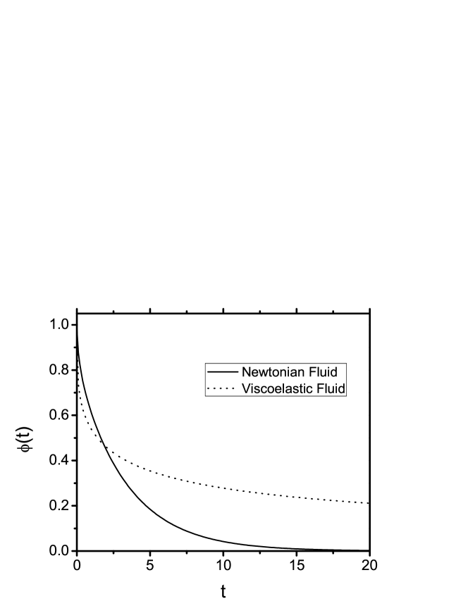
Figure 1: $\phi(t)$ against time ($t$). The values of parameters used are: $N=100,b=0.1,\xi=1,k_{B}T=1$.

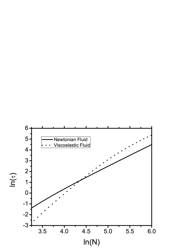
Figure 2: $ln(\tau)$ against $ln(N)$. The values of parameters used are: $a=0.5,b=0.1,\xi=1,k_{B}T=1$.

VI conclusions

In this paper we calculate the looping time for a chain immersed in a viscoelastic fluid where the mean square displacement of the center of mass of the chain scales as $t^{1/2}$. We found that up to a chain length viscoelastic fluid actually enhances the looping rate as compared to a Newtonian fluid with the same friction. But beyond a chain length the trend is reversed. This observation is due to the faster short time decay of the normal modes of the chain in the viscoelastic fluid as compared to in a Newtonian fluid. This is eve more prominent for short chains. Also no scaling of the looping time with the chain length seems to exist in viscoelastic fluid. Here we would like to point out that in a real viscoelastic fluid a chain would definitely feel a larger frictional drag. Thus in a real viscoelastic fluid the chain would relax even slower and one would expect slower looping time as compared to normal Rouse chain even with short chains.

In future we would like to investigate the effect of self interaction along with the viscoelastic background on the looping dynamics. It is obvious that in a crowded environment self interactions will also have profound influence on the looping dynamics of the chains.

VII acknowledgement

This work was carried out during the author’s stay at the Indian Institute of Science and supported by the Department of Science and Technology through the J. C. Bose fellowship project of K. L. Sebastian. The author thanks K. L. Sebastian for encouragements.

References

- Wilemski and Fixman (1974) G. Wilemski and M. Fixman, J. Chem. Phys. 60, 866 (1974).
- Doi (1975) M. Doi, Chem. Phys. 9, 455 (1975).
- Szabo et al. (1980) A. Szabo, K. Schulten, and Z. Schulten, J. Chem. Phys. 72, 4350 (1980).
- Srinivas et al. (2002) G. Srinivas, B. Bagchi, and K. L. Sebastian, J. Chem. Phys. 116, 7276 (2002).
- Thirumalai and Hyeon (2005) D. Thirumalai and C. Hyeon, Biochemistry 44, 4957 (2005).
- Toan et al. (2008) N. M. Toan, G. Morrison, C. Hyeon, and D. Thirumalai, J. Phys. Chem. B 112, 6094 (2008).
- Buscaqlia et al. (2005) M. Buscaqlia, J. Kubelka, W. A. Eaton, and J. Hofrichtev, J. Mol. Biol. 347, 657 (2005).
- Hudgins et al. (2002) R. R. Hudgins, F. Huang, G. Gramlich, and W. M. Nau, J. Am. Chem. Soc. 124, 556 (2002).
- Friedman and O’Shaughnessy (1989) B. Friedman and B. O’Shaughnessy, Phys. Rev. A 40, 5950 (1989).
- Chakrabarti (2012) R. Chakrabarti, Physica A DOI:10.1016/j.physca.2012.03.025 (2012).
- Santo and Sebastian (2009) K. P. Santo and K. L. Sebastian, Phys. Rev. E. 80, 061801 (2009).
- Dua and Cherayil (2002a) A. Dua and B. J. Cherayil, J. Chem. Phys. 116, 399 (2002a).
- Dua and Cherayil (2002b) A. Dua and B. J. Cherayil, J. Chem. Phys. 117, 7765 (2002b).
- Hyeon and Thirumalai (2006) C. Hyeon and D. Thirumalai, J. Chem. Phys 124, 104905 (2006).
- Debnath and Cherayil (2004) P. Debnath and B. J. Cherayil, J. Chem. Phys. 120, 2482 (2004).
- Ernst et al. (2012) D. Ernst, M. Hellmann, J. Kohler, and M. Weiss, Soft Matter DOI: 10.1039/c2sm25220a (2012).
- Weber et al. (2010a) S. C. Weber, A. J. Spakowitz, and J. A. Theriot, Phys. Rev. Lett 104, 238102 (2010a).
- Jeon et al. (2011) J.-H. Jeon, V. Tejedor, S. Burov, E. Barkai, C. Selhuber-Unkel, K. Berg-Sørensen, L. Oddershede, and R. Metzler, Phys. Rev. Lett. 106, 048103 (2011).
- Weber et al. (2010b) S. C. Weber, J. A. Theriot, and A. J. Spakowitz, Phys. Rev. E 82, 011913 (2010b).
- Schweizer (1989) K. S. Schweizer, J. Chem. Phys 91, 5802 (1989).
- Doi and Edwards (1988) M. Doi and S. F. Edwards, The Theory of Polymer Dynamics (Clarendon Press. Oxford, 1988).
- Kawakatsu (2004) T. Kawakatsu, Statistical Physics of Polymers An Introduction (Springer, 2004).
- Redner (2001) S. Redner, A Guide to First Passage Processes (Cambridge University Press, Cambridge UK, 2001).
- Chakrabarti and Sebastian (2009) R. Chakrabarti and K. L. Sebastian, J. Chem. Phys. 131, 224504 (2009).
- Sebastian (1992) K. L. Sebastian, Phys. Rev. A. 46, R1732 (1992).
- Debnath et al. (2006) A. Debnath, R. Chakrabarti, and K. L. Sebastian, J. Chem. Phys. 124, 204111 (2006).
- Chakrabarti (2010) R. Chakrabarti, Chem. Phys. Lett. 495, 60 (2010).
- Sokolov (2003) I. M. Sokolov, Phys. Rev. Lett. 90, 080601 (2003).
- Pastor et al. (1996) R. W. Pastor, R. Zwanzig, and A. Szabo, J. Chem. Phys. 105, 3878 (1996).
- Min et al. (2005) W. Min, G. Luo, B. J. Cherayil, S. C. Kou, and X. S. Xie, Phys. Rev. Lett 94, 198302 (2005).
- Min and Xie (2006) W. Min and S. Xie, Phys. Rev. E 73, 010902 (2006).
- Chakrabarti (2007) R. Chakrabarti, J. Chem. Phys. 126, 134106 (2007).
- Erdèlyi et al. (1993) A. Erdèlyi, W. Magnus, F. Oberhettinger, and F. G. Tricomi, Higher Transcendental Functions, Vol. 3 (McGraw-Hill New York, 1993).