Ricci focusing, shearing, and the expansion rate in an almost homogeneous Universe
Abstract
The Universe is inhomogeneous, and yet it seems to be incredibly well-characterised by a homogeneous relativistic model. One of the current challenges is to accurately characterise the properties of such a model. In this paper we explore how inhomogeneities may affect the overall optical properties of the Universe by quantifying how they can bias the redshift-distance relation in a number of toy models that mimic the real Universe. The models that we explore are statistically homogeneous on large scales. We find that the effect of inhomogeneities is of order of a few percent, which can be quite important in precise estimation of cosmological parameters. We discuss what lessons can be learned to help us tackle a more realistic inhomogeneous universe.
1 Introduction
Large scale redshift surveys of galaxies reveal a hierarchy of structure that extends out to hundreds of Megaparsecs, yet a homogeneous cosmological model lies at the core of our understanding of how the Universe evolves. Such an assumption works incredibly well, as can be seen from current analyses of the Cosmic Microwave Background (CMB). The linearly perturbed Friedmann–Lemaître–Robertson–Walker (FLRW) model can fit observations of the CMB with exquisite precision [1].
Nevertheless we cannot avoid the fact that the Universe is inhomogeneous, especially on small scales. Indeed, as a first approximation, space looks empty, with nuggets of mass and energy clustered together to form an intricate cosmic web. It is quite possible that the smooth description of space emerges as the average behaviour of a fundamentally inhomogeneous universe (cf. [2, 3, 4, 5]). This is an operation that we are familiar with closer to home, when we describe a gas or liquid through their macroscopic properties instead of through a detailed atomistic description. We would like to be able to do the same for the Universe, i.e. to infer the smooth, large scale (macroscopic) properties of space time from cosmological observations without having to worry about the discreteness of its constituents on small scales. We attempt to reconcile such an observation with a homogeneous universe by saying that our local, granular point of view is merely the small scale limit of the description given by the -Cold Dark Matter (CDM) cosmology. We then assume that on large scales, CDM is accurately described by a smooth cosmological fluid which on small scales fragments into particle dark matter and forms halos. Some have expressed strong concerns about the validity of such an approach (cf. [6, 7, 8]), especially because it is not clear whether the inhomogeneities on small scales will radically affect the large scale dynamics of the Universe (see [9] – [27], but see also [28, 29, 30] for counterexamples).
There are a number of interesting and important issues that must be addressed when tackling this problem. In this paper we wish to focus on one: how inhomogeneities can affect the inferred optical properties of the Universe. This problem has been looked at before, throughout the 1960s [31] – [37] and 1970s [38] – [40], and more recently [41] – [75], with a variety of different assumptions and results.
In this paper we look at how different effects can modify the redshift-distance relation, (, ). One might expect, a priori, that studying the effect of inhomogeneities on (, ) is pointless: in 1976, Weinberg [40] claimed that the overall (, ) for an inhomogeneous Universe should, on the whole, match that of the average homogeneous Universe. Views are somewhat divided on the validity of Weinberg’s argument and its generality, with cosmologists tending to accept it wholesale, while some relativists are slightly more sceptical and question its assumptions (cf. [76]). In this paper we will be completely agnostic.
Our approach is based entirely on the Sachs equations. Within the framework of these equations, we study different aspects of the redshift-distance relation. This is a complementary procedure to what is usually done111The most commonly-implemented procedure to account for the effect of inhomogeneities on light propagation is the magnification matrix approach. In almost all cases, one further assumes that light propagates on unperturbed geodesics, and thus the redshift (to a source located at some fixed comoving distance) is calculated as in the background homogeneous models, while inhomogeneities only affect the magnification/demagnification (for theoretical analysis see [42, 52, 72], or for practical implementation in ray tracing codes see [49, 50, 73]).. Our approach will be to use a number of different approximate models: high resolution N-body simulations, halo models, and a variety of swiss cheese models with Lemaître-Tolman-Bondi inhomogeneities.
While what we find is not, as yet, definitive, it does shed light on how important the effects of inhomogeneities might be. The paper is structured as follows. In Section 2 we present the Sachs equations and their various limits. In Section 3 we look at the effect of Ricci focusing, in Section 4 we study the impact of shear, and in Section 5 we attempt to include local fluctuations in the expansion rate. In each of these sections, we need to consider different models for inhomogeneities. In Section 6 we discuss our results.
2 Distance redshift relation
The Sachs optical equations describe the evolution of optical quantities, the expansion of the null bundle and its shear [31]
| (1) | |||
| (2) |
where and are respectively the Ricci and Weyl tensors, is the null vector and is perpendicular to and is confined to a surface tangent to a wave front. In the gravitational lensing nomenclature, ‘shear’ normally refers to the image distortion . These two quantities are related but are not the same, and in order to avoid any confusion, we will always refer to as to the shearing (for a detailed set of equations that relates these two quantities, see [69]).
The rate of change of the distance depends on the expansion rate of the light bundle in such a way that the angular diameter distance, , satisfies
| (3) |
Recall that the luminosity distance is given by [77, 78]. Rewriting equation (1), we find that
| (4) |
We need a set of initial conditions to solve for (, ), but more importantly we also need: (1) the Ricci curvature ; (2) the Weyl curvature ; (3) the transformation from the affine parameter to the redshift .
Using the Einstein equations () (where and is the gravitational constant), with the energy momentum tensor of a perfect fluid, one has that
| (5) |
In comoving coordinates, using the definition of redshift (where the subscripts and refer to the instants of emission and observation, respectively), one obtains
| (6) |
where we have used the freedom of the affine re-parametrization222The affine parametrization is conserved with respect to linear transformations, [79]. to set . For the case of dust (pressureless matter), the Ricci focusing depends only on matter density along the past null cone. From now on, we focus only on this case (dark matter can be treated as being pressureless, and for the cosmological constant we have ), i.e. we assume that the Ricci focusing is given by
| (7) |
Unfortunately, there is no ‘easy’ trick for estimating the Weyl focusing, and so to calculate this factor one has to solve for the null geodesics. In fact, solving null geodesics is also important for linking with , which can be done by using the redshift formula together with the null geodesic equations. In comoving coordinates, we have
| (8) |
which allows us to link with . In a homogeneous space time we have
| (9) |
where is the Hubble rate, and one recovers the textbook redshift-distance relation. If one assumes that where , the Dyer-Roeder formula is recovered [38, 39].
3 The role of Ricci focusing
We will first try to quantify the effect of Ricci focusing. To do so, we need to solve (4) in terms of , and . In this section, we assume that and are exactly the same as in the background FLRW model [see the first two terms in (9)]. We wish to study ‘realistic’ density profiles along the line of sight, and to do so we use density fields from the Millennium simulation [80, 81].
The Millennium simulation is an N-body simulation of the concordance cosmology. It consists of 10,077,696,000 particles of mass within a cube of volume Mpc. The simulation was performed using the GADGET-2 code [82]. In our calculations, we use the Millennium MField, which is the dark matter density field put on a grid, smoothed with Gaussian kernels 333, where of size: 1.25 Mpc, 2.5 Mpc, 5 Mpc, and 10 Mpc, labelled , , , and respectively. We randomly place an observer in the Millennium box, and then calculate different lines of sight (each in a different direction from the observer, and for each line of sight we randomly select a different observer). We assume periodic boundary conditions, so that when the light ray exits the Millennium box, it enters the other side of the box with entry angles the same as the exit angles (to enforce periodic boundary conditions). Since the MField consists of density maps on discreet time slices, to get at any required instant we interpolate between different time slices.
We calculate the light propagation out to , solve Eq. (4) and then write the distance as a deviation from the expected value in the background model (in our case the CDM model),
| (10) |
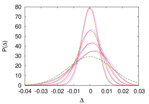
Results in terms of the probability distribution function (PDF) of are presented in Fig. 1. We find that the larger the smoothing radius, the smaller the variance: for the standard deviation is (uppermost solid curve in Fig. 1); for the standard deviation is (the solid curve second from the top in Fig. 1); for the standard deviation is (the solid curve third from the top in Fig. 1); and for the standard deviation is . It is interesting to compare these results with the ones obtained using the weak lensing formula (in the Born approximation),
| (11) |
where is the comoving coordinate, and we use the same as before. The results are plotted with dotted lines in Fig. 1. As shown, the PDFs are very similar to the ones obtained within the Ricci focusing regime. Finally, we calculate the standard deviation by squaring the expression above (where the mean is zero by construction) and replacing with the matter power spectrum [83],
| (12) |
In this case, the standard deviation of the distance correction is444Here, in order to compare with the Millennium simulation, we use the cosmological parameters that were used in the Millennium simulation. If the WMAP7 set of cosmological parameters is used instead, then . (the dashed curve in Fig. 1 is the Gaussian PDF with mean of zero and standard deviation of ).
The above results clearly reveal a pattern. First of all, the smaller the smoothing radius, the larger the variance, although even with the 1.25 Mpc smoothing radius we get a smaller standard deviation than was obtained within the framework of linear approximation. Also, note that the maximum of the PDF lies on the demagnification side (i.e. ), so a random object is most likely to be dimmer than on average. Nevertheless, in all cases the mean is almost zero: , , , , for , , , and respectively555Note that, for each different line of sight, we chose a different observer location. If we located an observer inside some deep inhomogeneity instead, such as a void of , , , , then the mean would be , , , . This suggest that the effect of local inhomogeneity on the distance (to in our case) is of order . In this paper we try to avoid the ‘local’ effects introduced by nearby inhomogeneities, so that we have a more clear insight to light propagation effects alone. For papers that study the local bias see [84]–[89].
4 The role of smoothing and Weyl focusing
We now extend our analysis to investigate the role of smoothing and the effect of Weyl focusing on the optical properties of the Universe. When dealing with the Weyl focusing, it is not straightforward to link density fields with the Weyl curvature. An ideal situation would be to have an exact generic solution of the Einstein field equations, and use that to model the evolution and effects of the Weyl curvature. Since there is no such a solution, in practise we must always employ some approximations. Here we will evaluate the Weyl focusing within the halo model.
Simply put, the halo model considered here consists of a universe filled with different halos of masses above , while the rest of the mass density (in objects of masses below this threshold) is assumed to be distributed homogeneously. The halo model we use closely follows the construction outlined in detail in Ref. [64]. Each halo is described by the Navarro-Frenk-White (NFW) density profile [90],
| (13) |
where is the radius of the halo, defined as
| (14) |
with , and (the halo is defined as an overdensity of mass , whose constant density contrast is 180 with respect to the mean matter density, cf. [91, 64]). Integrating , and using the expression above, one finds that
| (15) |
where is the concentration parameter, whose evolution given in [92] as
| (16) |
The number density of halos at a given instant in time is given by the halo mass function
with and given by [91]
| (17) |
where is the growth factor (this is usually written as , but we use here in order to avoid confusion with distance).
The halo model allows us to address the problem of smoothing — instead of dealing with a continuous density field, we now have a discrete set of dark matter halos — although one should keep in mind that, given the characteristics described above, this is not really a completely ‘discrete’ model. It also allows us to take into account the effect of the shearing, by assuming that the Weyl focusing for a particular halo, , is calculated using the Lemaître–Tolman (LT) model [93, 94] (an exact general relativistic model of an spherically symmetric, inhomogeneous, non-stationary space time) [47, 48]
| (18) |
where is the impact parameter, is the areal radius,
We apply the weak field approximations (cf. Ref. [33]) and assume that the total Weyl focusing is a sum over all contributors, . Note that, outside the halo, , and so only halos that are close to the light ray contribute most significantly.
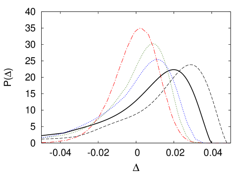
We again solve Eq. (4) for different lines of sight. The Ricci and Weyl focusing are calculated using the halo model, while is assumed to be the same as in the FLRW background model [see the first term of (9)]. The resulting distribution for is presented in Fig. 2 (thick solid curve). As expected, the variance is much larger than when the smoothed Millennium maps were used. Also, the maximum is shifted more towards positive values of . The mean, as before, is still negligible, at .
For comparison, and to gain a better understanding of the different factors, we now consider rather unphysical variations of the halo model. The first variation is when we neglect the shearing – when solving (4), we put . The result of this is shown as the dashed line in Fig. 2. As can be seen, it is significantly shifted to the magnification side (positive ) – the mean is . This shows that, when considering the halo model, the role of the shearing should not be neglected when calculating the distance correction.
To better understand the relation between the halo model and the smoothed Millennium density fields, we can study two more unconventional modifications of the halo model. In order to reduce the level of discreteness of the halo model, we decrease the value of the parameter , which results in larger halos and a lower amplitude of the halo density profiles. In the first case we reduce to , which means that the radius of the halo increases by roughly . In the second case, we reduce to , which results in a increase in the halo’s radius666For example, a halo of mass and has kpc [this follows from (14)], for and , kpc and kpc respectively.. We plot these results as dotted lines in Fig. 2. As can be seen, when we increase the halo radii (and hence decrease the degree of discreteness), we approach the results obtained when using the smoothed Millennium maps.
So far, the results reveal the same pattern: a skewed distribution with a maximum at the demagnification side (). This can easily be understood within the framework of the weak lensing formula (11): when light rays pass through the large-scale structure, they are more likely to propagate through voids than through more dense, compact structures. Therefore, it is more likely to have along the line of sight and, as follows from (11), . This is clearly visible when we use the smoothed Millennium maps. If the smoothing scale is sufficiently large, the resulting density field approaches a Gaussian field (all non-linearities are washed away, and we recover symmetry between overdense and underdense regions), and so the maximum approaches zero (for pure Gaussian fluctuations ). In the halo model, we deal with halos that are very compact and occupy a relatively small volume, which makes propagation through voids even more likely to occur. We therefore see a shift of towards higher demagnification (see Fig. 2). Occasionally, light rays pass close to a halo, and then both the Ricci and Weyl focusing magnify the light bundle. Thus, on average, the total balance is recovered, and the mean of is almost zero (in the lensing framework, as seen in (11), due to matter conservation it is exactly zero). Here we find a mean of order . A small deviation from the expected value in the FLRW model is expected. For example the analogue of the Integrated Sachs-Wolfe effect will affect the redshift, and thus . Also, the local environment plays a role – note that our observer is located inside an inhomogeneity (i.e. not within a homogeneous region) – see footnote on page 6.
The same pattern has also been reported in previous studies – see for example in [42], and in ray tracing though N-body simulations. In fact, our halo model provides very good agreement with the ray tracing through the Millennium simulation, cf. [49, 50]. It is also in almost perfect agreement with the PDF generated using the turboGL code[59, 64]777The turboGL code uses the halo model to calculate the PDF of the weak lensing convergence. The effect of the shear is neglected in turboGL. However, if the zero-shear PDFs are compared, they are in agreement. Note that, as seen in Fig. 2, the zero-shear PDF, apart from a small change in its amplitude, looks like the translation of the nonzero-shear PDF..
The results are therefore consistent with the most commonly-implemented procedures, where the effects of inhomogeneities on light propagation are calculated using the magnification matrix approach. In almost all cases, one further assumes that light propagates on unperturbed geodesics, and so the redshift (to a source located at some fixed comoving distance) is calculated as in the background homogeneous models, while inhomogeneities only affect the magnification/demagnification. So far, we have been doing the same (that is, we assumed that is the same as in the background FLRW model). We therefore examine the effect of changing in the next section.
5 The role of the non-uniform expansion rate
The last effect that remains to be examined is related to . So far we have been applying the FLRW formula, but as shown in (8), to calculate it correctly we need to solve null geodesics. We now address this point by studying light propagation within the LT Swiss Cheese model. The advantage of the LT model is that it is an exact model, and so no approximations are required when modelling the light propagation, evolution of perturbations, or the Weyl curvature. The disadvantage is that each particular inhomogeneity must be spherically symmetric, and we do not have the freedom to mimic the Millennium density profile. Furthermore, we cannot describe virialised objects such as massive matter halos (we will come back to this point later on).
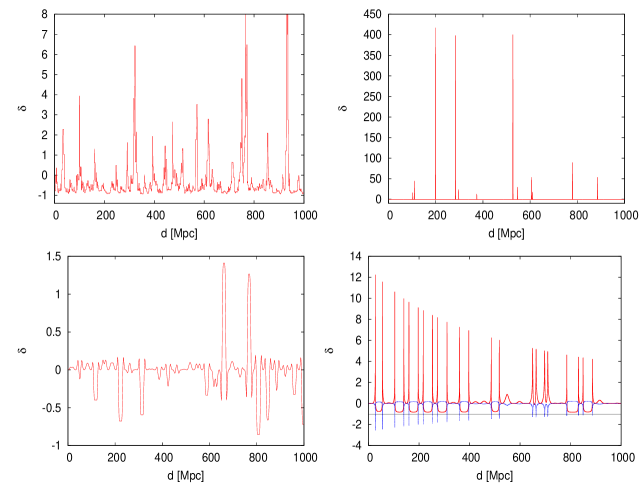
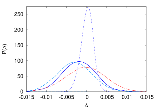
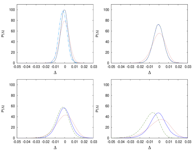
Let us first consider a ‘mild’ Swiss Cheese model, i.e. one without large density fluctuations. Each inhomogeneity has a radius of Mpc, beyond which the system becomes homogeneous. The density contrast inside the inhomogeneity is generated using the log-normal PDF111, where , and ., with (i.e. Mpc). An example of a random line of sight through this model is presented in the panel to the lower left of Fig. 3. Within this model, we solve the null geodesic equations using (8) to obtain . The Weyl focusing is calculated from (18) and the distance is calculated by solving (4). In order to avoid effects of local structures, we place the observer and the source within the homogeneous regions. The resulting PDF of for a source at is presented in Fig. 4 (dotted line). The mean is . Qualitatively, the results are very similar to the ones obtained before: the PDF is skewed, with the maximum at the positive side of . Quantitatively, however, the variance is much smaller than in previous cases. This is because of the smaller amplitude of inhomogeneities along the line of sight, which can be seen by comparing the upper left (Millennium) and upper right (halo model) panels of Fig. 3 to the lower left panel of Fig. 3 (the ‘mild’ Swiss Cheese case).
To bring us closer to the Millennium case, but in such a way as to include shearing and a modified relation, we now consider a more ‘realistic’ model, with large deep voids (with, for example, a present day radius of Mpc and a density contrast of ). These voids have highly non-linear walls which, due to the high density contrast, are at the collapsing stage, clearly visible in the lower right panel of Fig. 3 (dotted line). The PDF obtained within this model is presented in Fig. 4 (solid line). The mean is . The first qualitative difference is that the maximum is now at negative (magnification). Secondly, due to large fluctuations in the density field, the variance is larger, and is comparable with the Millennium density field (dotted-dashed line in Fig. 4).
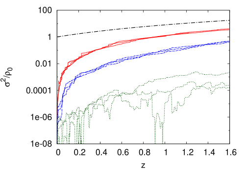
The surprising result is that the maximum is on the magnification side (). Such a phenomenon has not been reported before. Let us closely examine what could lead to such an unexpected behaviour. Three working hypotheses can be put forward to explain this: (1) the effect of the Weyl focusing, (2) the problem with collapsing regions, (3) an artefact of the symmetry of the density contrast. With regards to the shearing, we have seen in the previous section, when comparing the halo model with and without the Weyl focusing, that if , the PDF shifts to lower values of . However, as seen from Fig. 5, the role of the Weyl focusing for our Swiss Cheese models is small (cf. [70] and [72] for a similar conclusion regarding the role of the Weyl focusing in this type of model). Essentially, if the density contrast is not high (unlike in the halo model; compare the upper right panel of Fig. 3 with the lower right panel), the role of the Weyl focusing is small (compare the set of 3 solid lines with the set of 3 dashed or dotted lines in Fig. 5). We therefore conclude that the shear cannot be responsible for the shift of from demagnification to the magnification side. This can be confirmed by re-running the same model with set to zero – the resulting PDF is exactly the same as in the case of (solid line in Fig. 4).
Our second hypothesis involves considering the role of collapsing regions. In this case, , which may strongly affect . In the real Universe, whenever the density field has a high amplitude, cosmic structures are virialised, and hence they are not collapsing. Unfortunately, there is no rotation within the LT model, which could prevent the collapse. Therefore, as seen in the lower right panel of Fig. 3, the expansion is negative within the wall. In order to ‘correct’ the model for the virialisation effect, whenever the expansion rate is negative, we assume that the structure is already virialised and so the redshift does not change within this region. That is, we assume that in these regions, whereas in all other regions we use the exact formula, i.e. . We should exercise caution when analysing these results, as this ‘correction’ was done by hand. The fact that some regions are virialised, and hence , is not a consequence of a model, and so there is clearly an issue of self-consistency. The resulting PDF is presented using a dashed line in Fig. 4, where we find that the maximum of the curve is shifted even further towards negative values of . The mean is almost twice as large as before, . Clearly this does not explain why , and in fact it makes things even ‘worse’.
Our final hypothesis concerns the symmetry of the density perturbations. We can already see that this cannot be the cause, as for the ‘mild’ Swiss Cheese model. Nevertheless, we return to the Millennium smoothed maps and perform further tests. We proceed as before, with the only difference being that, when solving , we no longer assume a uniform expansion rate as in (9), but instead assume that
| (19) |
where is the expansion rate of the background model. In general
where is the matter scalar of the expansion and is the shear of the matter velocity field. We further work under the assumption of zero shear and so we only consider fluctuations in the expansion field, which in the linear regime are given by
| (20) |
Here, is the growth function, . This method has thus 2 limitations, and works well as long as (1) the density contrast is not too high and (2) the matter shear is negligible. We proceed further with this toy model, as it will bring more insight into results obtained within the exact LT model.
Naively, one can think of this as follows: because , we should expect (qualitatively) the same results as before, except for a potentially larger variance due to the presence of both and . Our results are presented in Fig. 6. First of all, the variance changes only slightly. Secondly, and most importantly, we find that . In the case (with 10 Mpc smoothing scale), the results are strongly comparable with our non-linear Swiss Cheese model; for comparison we present its PDF in the upper left panel of Fig. 6 (dot-dashed line). Also, the mean of is of the same order of magnitude as in the Swiss Cheese model, i.e. — see Table 1.
Finally, as before, we try to ‘correct’ the model for the effects of virialization. As seen from (20), if
then such a region collapses. In the case, almost of regions have a density contrast above this threshold (see Table LABEL:tab2). As before, we set
In this case, if we calculate the average , due to the fact that we neglect the most negative contributions, the average is no longer zero, and in the case of the average is approximately (it can only be zero if ). The resulting PDFs are presented in Fig. 6 (dashed lines). As in the case of the non-linear Swiss Cheese model before, the PDF shifts towards even more negative values of . For detailed values of the means of the PDFs, see Table 1.
| Model | |||
|---|---|---|---|
| mild Swiss Cheese | |||
| non-linear Swiss Cheese | |||
| halo |
| Map | of | |
|---|---|---|
Proceeding further with the idea of a variable expansion rate and its impact on , we also recalculate our results for the halo models that were considered previously. Since halos are virialised, their interiors are set to . The resulting PDF is presented in the right panel of Fig. 7. As was the case for the Millennium maps, a shift towards magnification is evident. This should be compared with the mild Swiss Cheese model, or with the models which assumed a uniform expansion rate, where the PDF peaked on the positive side of .
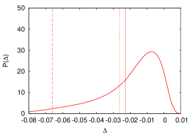
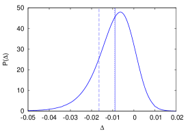
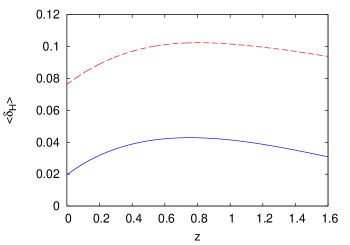
In Secs. 3 and 4 we assumed that was the same as in the FLRW background model. As a result, we found that . For the Swiss Cheese model, we had variations in with regards to the background, but still found that . It was only when we started to ‘correct’ our models for virialization that we found deviations of order of (for the halo and models). We now want to follow this up further, and test how the average of the distance follows the background’s . Note that when we ‘force’ some regions not to collapse (by setting whenever ), we change the average expansion history (see Table LABEL:tab2 and Fig. 8), and thus also . This leads us to question: if we recover the average correctly, will we obtain the correct mean of the distance, without the need for a detailed calculation of the Ricci and Weyl focusing?
We study this issue within the halo and models, as they have the largest deviation of . The PDFs obtained within these models are presented in Fig. 7. The mean of is shown as a vertical solid line. The average of the expansion rate fluctuations calculated on a slice of constant is presented in Fig. 8. Before proceeding further, we must comment on one important aspect of our computations. Cosmologists tend to use the redshift as a proxy for time, so they express the evolution of different fields in terms of the redshift, for example:
| (21) |
Only in the case of perfect homogeneity do we have that (the proxy for time, i.e. the redshift of a photon at a given time in a perfect homogeneous model) coincides with (the actual shift of the photon’s frequency). Thus, in solving the Sachs equations, one must solve the following:
| (22) |
We solve these, and plot the results as dotted lines in Fig. 7. As can be seen, the difference between the actual value, and that obtained from the above set of equations, is of order of , (as before, where we set to its value in the background CDM model). For comparison, we solve the above equation with
This time, the result (given by the dashed line) is significantly displaced to the left. The reason for the shift towards higher magnification is that if then, as follows from (22), we have that , and so if we replace with , we increase the Ricci focusing, hence higher magnification. This simple exercise shows that if one is interested in having an average without having to worry about the Ricci or Weyl focusing, one can simply use the average of one’s model. Caution must be taken, though, when studying models in which is not proportional to . Such models include, for example, Gpc-scale inhomogeneous LT models222In fact the results of this paper provide a fresh view into different configurations of the LT model, which consist of giant voids [95, 96] and giant humps [97]. Within the giant voids increases outwards, which results in the decrease of the expansion rate along the past null cone, hence the dimming of the supernova within the giant voids is caused by the change of the relation. Whereas for the giant hump models decreases outwards making the Ricci focusing less efficient, and hence causing additional dimming. and some backreaction models.
In this section we have tested all 3 factors that affect the relation between and via the Sachs equation: , , and . In order to model them in a self-consistent manner, we used the LT Swiss Cheese model. In all cases, we found that the distance does not change, on average, by more than (at ). This result is fairly consistent with what has been found by other groups who have employed exact models, and ensured the proper randomization of light rays333Note that for models where the distance correction is calculated using the Born approximation, have by the construction [52, 59, 64, 72] (cf. [47, 48, 56, 70, 74, 75]).
Our main motivation has been to follow, as closely as possible, the standard procedures to test self-consistency and the impact of inhomogeneities on the optical properties of the Universe within models that follow the FLRW evolution. Nevertheless, it is not completely obvious that one should recover the FLRW results for these models, unless one completely agrees with Weinberg’s reasoning. If one does take Weinberg’s results at face value, then our results should be considered as a big deviation, about two orders of magnitude larger than what is allowed by the analogue of the Integrated Sachs Wolfe effect (which should be of order ).
From one point of view, our results have turned out to be quite surprising. In the case of large fluctuations in the density and expansion fields, the mode of shifts to the magnification side. Such a behaviour has not been reported before. The effect is only visible if the degree of inhomogeneity is large – for small amplitude Swiss Cheese models, we recover the standard results. This can be explained using the same ‘voids argument’ that we used in the case of the weak lensing approximation – since the structures in the Universe form a cosmic web, it is more likely for photons to propagate through voids (hence the position of the mode is associated with the amount of void regions). As seen from (11), the weak lensing regime is only sensitive to density fluctuations, and so the mode is positive. If we introduce fluctuations in the expansion rate, then the redshift decreases, as seen from (19). Hence an object located at the same distance has a higher redshift, and thus gives the impression of being magnified compared to the homogeneous case444The same fact can also be visualised in terms of the slope of the relation – when the redshift increases faster than in the homogeneous case, the slope decreases. See, for example, Fig. 4 of [74], which shows the change of the slope in the relation , depending on fluctuations in the density and expansion rate.. This is the reason why the mode is now on the magnification side.
A valid point, and one worth further investigation, is related to the fact that, due to the virialisation of high density regions, the average expansion rate may deviate from the background value. This was already pointed out in [98, 99] in the context of backreaction models, although as shown in [100, 101], the presence of matter shear may decrease the backreaction effect, leaving the evolution of the average quantities relatively unchanged. Nevertheless, in such cases, the 3D volume average on surfaces of constant time may not coincide with the average on slices of constant . As a result, as we have shown above, we would still expect a change in the redshift-distance relation. However, we reiterate that care should be taken in interpreting these results – changing by hand may not lead to self consistent results (although keeping the expansion rate uniform may also turn out to be inconsistent). To test this phenomenon more closely, we require exact models that allow for virialisation. The LT models are definitely not suitable for such a study.
6 Conclusions
The overarching question that we wish to address is: does the FLRW model, which correctly describes the evolution of the background, correctly recover (on average) the distance-redshift relation? Our results, while not entirely conclusive, are suggestive. We have explored a suite of models which are inhomogeneous, but close to the FLRW. We find that, if the background model correctly describes the evolution of the average expansion rate and the average matter density, then indeed the homogeneous model is a good approximation.
Our results show that Ricci focusing alone introduces deviations from the average value. The PDF is skewed and the maximum is on the demagnification side (a random object will most likely be dimmer than the average). The change of the mean is negligible, which means that, on average, distances coincide with the expected distance in the background model. The deviation from the average (for a particular line of sight) depends crucially on the smoothing scale and, unsurprisingly, the smaller the smoothing scale, the larger the deviation. We find that Weyl focusing is important for objects with very high density contrast, and yet even in this case, the bias in the mean of is negligibly small.
We also find that the presence of large fluctuations in the expansion rate also affects the final results: there is a slight shift of the maximum of the PDF towards the magnification side (a random object will most likely be brighter than the average), and the variance changes. In particular, we find that if the average expansion rate deviates from the background expansion rate, the distance (on average) changes by a few percent. In the real Universe, such a situation may occur in the late non-linear stage of evolution, where large voids expand much faster than the background, while virialised over-dense regions do not expand at all (for these fluctuations to cancel each other, at some stage the presence of collapsing regions is required).
In summary, we have studied the various biases that cosmological inhomogeneities can introduce into the inferred optical properties of the Universe by considering a range of toy models. There are, of course, limitations to the accuracy and self-consistency of these models, and how well they mimic the real Universe. We find that the presence of inhomogeneities (around a fixed background) changes distances by at most a few percent, although the average is closely related to the background model. The only possible deviation of the average of the distance from the distance predicted by the background model is in situations where the background model does not correctly describe the evolution of the average quantities.
The lessons we have learned can be summarized in the form of a message to our readers. For cosmologists, we would like to point out that, with the increasing precision of cosmological observations, a change of few percent might soon become important for accurate estimation of cosmological parameters (cf. [63, 67]). In particular, the PDFs are skewed and hence, for a limited number of observational data, there might be a bias due to the fact that the mode does not coincide with the mean, or median. For relativists, we would argue that, to study the effect of inhomogeneities on observations, it is first important to understand how much inhomogeneities affect the evolution of the background model. Such a study should focus on and , and especially on potential deviations from (21), as this has the biggest impact on the distance-redshift relation (see, for example, Fig. 7 for a few percent change in the case where (cf. [68]). Thus, pinning down and will also provide the average of , without the need to account for the Weyl focusing or to model complex aspects of the Ricci focusing).
References
References
- [1] Komatsu E, Smith K M, Dunkley J, Bennett C L, Gold B, et al. Astrophys. J. Suppl. 192 18 (2011)
- [2] Lindquist R W, Wheeler J A, 1957, Rev. Mod. Phys. 29, 432; erratum 1959, Rev. Mod. Phys. 31, 839
- [3] Clifton T, Ferreira P G, 2009, Phys. Rev. D80, 103503; erratum 2011, Phys. Rev. D84, 109902
- [4] Clifton T, Ferreira P G, 2009, J. Cosmol. Astropart. Phys. JCAP10(2009)026
- [5] Clifton T, Ferreira P G, O’Donnell K, 2012, Phys. Rev. D85, 023502
- [6] Ellis G F R, 2011, Class. Q. Grav. 28 164001
- [7] Francesco Sylos Labini F, 2011, Class. Q. Grav. 28 164003
- [8] Krasiński, 2011, Acta Phys. Pol. B42 2263
- [9] Buchert T, 2000, Gen. Rel. Grav. 32 105
- [10] Buchert T, 2001, Gen. Rel. Grav. 33 1381
- [11] Wiltshire D L, 2007, New J. Phys. 9 377
- [12] Wiltshire D L, 2007, Phys. Rev. Lett. 99 251101
- [13] Bolejko K and Andersson L, 2008, J. Cosmol. Astropart. Phys. 11 003
- [14] Räsänen S, 2010, Phys. Rev. 81, 103512
- [15] Kolb E W, Marra V, Matarrese S, 2010, Gen. Rel. Grav., 42 1399
- [16] Krasiński A, Hellaby C, Bolejko K, Célérier M N 2010 Gen. Rel. Grav. 42 2453
- [17] Räsänen S, 2011, Class. Q. Grav. 28 164008
- [18] Roy X, Buchert T, Carloni S, Obadia N, 2011, Class. Q. Grav. 28 165004
- [19] Wiltshire D L, 2011, Class. Q. Grav. 28 164006 (2011)
- [20] Clarkson C, Umeh O, 2011, Class. Q. Grav. 28 164010
- [21] Buchert T, 2011, Class. Q. Grav. 28 164007 (2011)
- [22] Sussman R A, 2011, Class. Q. Grav. 28 235002
- [23] Clarkson C, Ellis G F R, Larena J, Umeh O, 2011, arXiv:1109.2314
- [24] Buchert T, Rasanen S, 2011, arXiv:1112.5335
- [25] Clarkson C, Clifton T, Coley A, Sung R, 2012, Phys. Rev. D85 043506
- [26] Bull P, Clifton T, 2012, arXiv:1203.4479
- [27] Hellaby C, 2012, J. Cosmol. Astropart. Phys. JCAP01(2012)043
- [28] Ishibashi A, Wald R M, 2006, Class. Q. Grav. 23 235
- [29] Green S R, Wald R M, 2011, Phys. Rev. D83, 084020
- [30] Clifton T, Rosquist K, Tavakol R, 2012, arXiv:1203.6478
- [31] Sachs R K 1961 Proc. Roy. Soc. London A 264 309
- [32] Zel’dovich Y. B., 1964, SvA, 8, 13
- [33] B. Bertotti, 1966, Proc. Roy. Soc. London A 294 195
- [34] Kristian J, Sachs R K 1966 Astrophys. J. 143 379
- [35] J. E. Gunn, 1967, Astrophys. J. 147, 61
- [36] J. E. Gunn, 1967, Astrophys. J. 150, 737
- [37] R. Kantowski, 1969, Astrophys. J. 155, 89
- [38] Dyer C. C., Roeder R. C., 1972, Astrophys. J. 174, L115
- [39] Dyer C. C., Roeder R. C., 1973, Astrophys. J. 180, L31
- [40] Weinberg S 1976 Astrophys. J. 208 L1
- [41] Kantowski R, Vaughan T, Branch D 1995 Astrophys. J. 447 35
- [42] Holz D. E., Wald R. M., 1998, Phys. Rev. D58 063501
- [43] Demiański M., de Ritis R., Marino A. A., Piedipalumbo E., 2003, Astron. Astroph. 411 33
- [44] Pyne T., Birkinshaw M., 2004, Mon. Not. R. Astron. Soc. 348 581
- [45] Bonvin C, Durrer R, Gasparini M A 2006 Phys. Rev. D D73 023523
- [46] Hui L., Greene P. B. 2006 Phys. Rev. D73 123526
- [47] Brouzakis N, Tetradis N, Tzavara E 2007 J. Cosmol. Astropart. Phys. JCAP02(2007)013
- [48] Brouzakis N, Tetradis N, Tzavara E 2008 J. Cosmol. Astropart. Phys. JCAP04(2008)008
- [49] S. Hilbert, S.D.M. White, J. Hartlap, and P. Schneider, 2007, Mon. Not. R. Astron. Soc. 382 121
- [50] S. Hilbert, S.D.M. White, J. Hartlap, and P. Schneider, 2008, Mon. Not. R. Astron. Soc. 386 1845
- [51] Ishak M, Richardson J, Garred D, Whittington D, Nwankwo A, Sussman R, 2008, Phys. Rev. D78 123531
- [52] Vanderveld R. A., Flanagan E. E., Wasserman I., 2008, Phys. Rev. D78 083511
- [53] Räsänen S., 2009, J. Cosmol. Astropart. Phys. JCAP02(2009)011
- [54] Valkenburg W 2009 J. Cosmol. Astropart. Phys. JCAP06(2009)010
- [55] Clifton T, Ferreira P G 2009 Phys. Rev. D80 103503
- [56] Clifton T, Zuntz J, 2009, Mon. Not. R. Astron. Soc. 400, 2185
- [57] Enqvist K., Mattsson M., Rigopoulos G., 2009, J. Cosmol. Astropart. Phys. JCAP09(2009)022
- [58] Bolejko K, 2009, Gen. Rel. Grav. 41 1737
- [59] K. Kainulainen, V. Marra, 2009, Phys. Rev. D80, 123020
- [60] Räsänen S., 2010, J. Cosmol. Astropart. Phys. JCAP03(2010)018
- [61] Mattsson T., 2010, Gen. Rel. Grav. 42, 567
- [62] Bolejko K, Célérier M-N, 2010, Phys. Rev. D82, 103510
- [63] Amendola L, Kainulainen K, Marra V, Quartin M, 2010, Phys. Rev. Lett. 105, 121302
- [64] Kainulainen K, Marra V, 2011, Phys. Rev. D83, 023009
- [65] Bolejko K, 2011, Mon. Not. R. Astron. Soc. 412 1937
- [66] Bolejko K, 2011, Astron. Astroph. 525 A49
- [67] Bolejko K, 2011, J. Cosmol. Astropart. Phys. 02 025
- [68] Rasanen S, 2011, arXiv:1107.1176
- [69] Clarkson C, Ellis GFR, Faltenbacher A, Maartens R, Umeh O, Uzan J-P, 2011, arXiv:1109.2484
- [70] Szybka S J 2011 Phys. Rev. D84 044011
- [71] Nwankwo A, Ishak M, Thompson J, 2011, J. Cosmol. Astropart. Phys. JCAP05(2011)028
- [72] Flanagan É É, Kumar N, Wasserman I, Vanderveld R A, 2012, Phys. Rev. D85 023510
- [73] Killedar M, Lasky P D, Lewis G F, Fluke C J, 2012, Mon. Not. R. Astron. Soc. 420 155
- [74] Meures N, Bruni M, 2012, Mon. Not. R. Astron. Soc. 419 1937
- [75] Di Dio E, Vonlanthen M, Durrer R, 2012, J. Cosmol. Astropart. Phys. JCAP02(2012)036
- [76] Ellis G F R, Bassett B A C C, Dunsby P K S 1998 Class. Quantum Grav. 15 2345
- [77] Etherington I M H, 1933, Phil. Mag. VII, 15, 761; reprinted, with historical comments, in 2007, Gen. Rel. Grav. 39 1055.
- [78] Ellis G F R, 1971, Proceedings of the International School of Physics ‘Enrico Fermi’, Course 47: General Relativity and Cosmology, ed. R. K. Sachs. Academic Press, New York and London, pp. 104 – 182; reprinted, with historical comments, in 2009, Gen. Rel. Grav. 41 581.
- [79] Plebański J, Krasiński A 2006 An Introduction to General Relativity and Cosmology (Cambridge: Cambridge University Press)
- [80] V. Springel et al. 2005, Nature 435, 629
- [81] M. Boylan-Kolchin et al. 2009, Mon. Not. R. Astron. Soc. 398, 1150
- [82] Springel V, 2005, Mon. Not. R. Astron. Soc. 364 1105
- [83] F. Bernardeau, L. Van Waerbeke, Y. Mellier, 1997, Astron. Astroph. 322 1
- [84] Romano A E, Chen P, 2011, J. Cosmol. Astropart. Phys. JCAP10(2011)016
- [85] Wiegand A, Schwarz D J, 2012, Astron. Astroph. 538, A147
- [86] Wiltshire D L, Smale P R, Mattsson T, Watkins R, 2012, arXiv:1201.5371
- [87] Valkenburg W, 2012, J. Cosmol. Astropart. Phys. JCAP01(2012)047
- [88] Valkenburg W, Bjaelde O E, 2012, arXiv:1203.4567
- [89] Marra V, Pääkkönen M, Valkenburg W, 2012, arXiv:1203.2180
- [90] J. F. Navarro, C. S. Frenk, S. D. M. White, 1996, Astrophys. J. 463 563
- [91] Jenkins A, Frenk C S, White S D M, Colberg J M, Cole S, Evrard A E, Couchman H M P, Yoshida N, 2001, Mon. Not. R. Astron. Soc. 321 372
- [92] A.R. Duffy, J. Schaye, S T Kay, and C. Dalla Vecchia, 2008, Mon. Not. R. Astron. Soc. 390 L64
- [93] Lemaître G 1933 Ann. Soc. Sci. Bruxelles A 53 51 (English translation, with historical comments: 1997 Gen. Rel. Grav. 29 637)
- [94] Tolman R C 1934 Proc. Nat. Acad. Sci. USA 20 169 (reprinted, with historical comments: 1997 Gen. Rel. Grav. 29 931)
- [95] Bolejko K, Krasiński A, Hellaby C, Célérier M-N,, 2009, Structures in the Universe by exact methods - formation, evolution, interactions, Cambridge University Press
- [96] Bolejko K, Célérier M-N, Krasiński A, 2012, Class. Q. Grav. 28, 164002.
- [97] Célérier M-N, Bolejko K, Krasiński A, 2010, Astron. Astroph. 518, A21.
- [98] Räsänen S, 2006, J. Cosmol. Astropart. Phys. JCAP0611(2006)003
- [99] Räsänen S, 2008, J. Cosmol. Astropart. Phys. JCAP0804(2008)026
- [100] Mattsson M and Mattsson T, 2010, J. Cosmol. Astropart. Phys. JCAP1010(2010)021
- [101] Mattsson M and Mattsson T, 2011, J. Cosmol. Astropart. Phys. JCAP1005(2011)003