The Role of Temperature in the occurrence of some Zeno Phenomena

B. Militello Dipartimento di Fisica dell’Università di Palermo, Via Archirafi 36, 90123 Palermo, Italy benedetto.militello@unipa.it
Abstract

Temperature can be responsible for strengthening effective couplings between quantum states, determining a hierarchy of interactions, and making it possible to establish such dynamical regimes known as Zeno dynamics, wherein a strong coupling can hinder the effects of a weak one. The relevant physical mechanisms which connect the structure of a thermal state with the appearance of special dynamical regimes are analyzed in depth.

pacs:
03.65.Xp, 03.65.Aa, 05.30.-d

I Introduction

In the last decades a lot of attention has been devoted to the role of temperature in quantum information and in quantum mechanics in general. In particular, the detrimental effects of an environment at finite or even high temperature have been studied in connection with many aspects of quantum mechanics. Nevertheless, many studies aimed at singling out robustness of quantum features even in the presence of high temperature, which for instance is the case of thermal entanglement. Recently, the connection between temperature and Quantum Zeno phenomena has also been explored.

The concept of quantum Zeno effect (QZE) — according to its original definition QZE consists in the inhibition of the dynamics of a physical system due to repeated “pulsed”  measurements ref:MishraSudarshan , which has been demonstrated in various systems ref:Itano1990 ; ref:Fischer1997 — has been progressively generalized. The first generalization consists in considering continuous measurements meant as dissipative processes ref:Schulman1998 , showing that a strong decay can be responsible for a dynamical decoupling that weakens the effects of other interactions ref:Panov1999a ; ref:Panov1999b ; ref:Militello2011 ; ref:Scala2010 . Another important generalization is related to the knowledge that even an additional coherent coupling can be responsible for diminishing the effects of other interactions, hence realizing the so called Zeno Dynamics ref:PascazioFacchi2001 ; ref:Militello2001A ; ref:Militello2001B and eventually leading to the concept of Zeno subspaces ref:PascazioFacchi2002 . Also pulsed interactions have been proven to be responsible for the formation of dynamically invariant subspaces ref:PascazioFacchi2004 ; ref:PascazioFacchi2008 ; ref:PascazioFacchi2010 .

Quantum Zeno effect has been exploited to develop applications in various fields, such as quantum information and nanotechnologies ref:App1 ; ref:App2 ; ref:App3 . Moreover, its importance in connection with fundamental concepts of quantum mechanics has been widely discussed ref:Home1997 . Nevertheless, Zeno phenomena are not confined to the realm of quantum mechanics, but, according to Peres, similar occurrences are possible even in classical mechanics ref:Peres1980 .

The connection between Zeno phenomena and temperature has been investigated by various authors. In 2002 Ruseckas analyzed the effects of thermalization of a measurement apparatus on the appearance and intensity of the quantum Zeno effect, showing that an higher temperature can amplify the power of pulsed measurements in inducing Zeno phenomena ref:Ruseckas2002 . In 2006 Maniscalco et al have studied the crossover between QZE and AZE — Anti-Zeno effect is the acceleration of the dynamics induced by measurements, usually incoming for short-but-not-too-short time intervals between subsequent measurements — in connection with the temperature of the bath the system under scrutiny is interacting with, showing that the QZE-AZE border can be significantly affected by temperature ref:Sabrina2006 . Recently, Scala et al have analyzed Landau-Zener (LZ) transitions in the presence of environmental effects, even in the case of a bath at finite or high temperature ref:ScalaLZ2011 . The analysis, developed through a master equation approach beyond the secular approximation, has shown that temperature can be responsible for a dynamical decoupling, which eventually leads to a Zeno effect. A subsequent study ref:MilitelloTQZE2011 developed in connection with a different physical situation — a simplified version of the previous problem, wherein a time-independent Hamiltonian has been considered in place of the LZ time-dependent coupling scheme — has shown that in some situations temperature can clearly contribute to induce a Zeno dynamics, weakening the effects of coherent couplings.

Starting from these results, one could wonder whether in those cases wherein temperature can influence more than one interactions it is possible to have temperature-dependent hierarchies of couplings, driving the appearance of Zeno behaviors. Indeed, for instance, if two or more interactions are strengthened by temperature, occurrence of Zeno phenomena could be obstructed, because of the impossibility of finding a coupling which is much stronger than others; in other cases temperature can enhance inhibition of the dynamics. In this paper we analyze the role of temperature when it affects more than one interactions, discussing appearance and disappearance of temperature-induced Zeno dynamics, and studying in depth the underlying physical mechanisms.

The paper is organized as follows. In section II we analyze the dynamics of a three-level system resonantly interacting with two harmonic oscillators initially prepared in a thermal state. In section III we extend the scheme by considering some detuning effects and show an interesting competition between detuning and temperature in determining Zeno regimes. In section IV we give some preliminary results that pave the way to the analysis of the case where many oscillators are involved in the coupling scheme. Finally, in section V we give some conclusive remarks.

II Zeno dynamics induced by Temperature

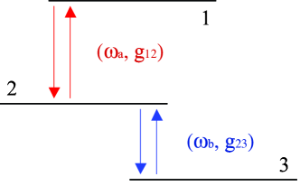
Let us consider a three-state system interacting with two harmonic oscillators initially prepared in a thermal state. The interaction with the oscillators can induce transitions from the upper state to the intermediate one and from the intermediate to the lowest. Both interactions are assumed to be resonant (see Fig. 1).

From general statements for the appearance of Zeno dynamics ref:PascazioFacchi2002 ; ref:PascazioFacchi2004 ; ref:Militello2001B , if the strength of the coupling between |2ket2\left|2\right\rangle and |3ket3\left|3\right\rangle is much greater than the strength of the other coupling, i.e. if |g23||g12|much-greater-thansubscript𝑔23subscript𝑔12|g_{23}|\gg|g_{12}|, then transitions from |1ket1\left|1\right\rangle to |2ket2\left|2\right\rangle — and vice versa — are hindered. Therefore, if the atomic system is initially prepared in the state |1ket1\left|1\right\rangle then the system does not evolve significantly.

We will show that this behavior occurs when temperature is high even if the condition |g23||g12|much-greater-thansubscript𝑔23subscript𝑔12|g_{23}|\gg|g_{12}| is not fulfilled, provided the frequency of the oscillator assisting 23232-3 transitions is much smaller than the frequency of the oscillator which couples |1ket1\left|1\right\rangle and |2ket2\left|2\right\rangle.

II.1 The Hamiltonian Model

Consider the following Hamiltonian model (=1Planck-constant-over-2-pi1\hbar=1):

H^=kωk|kk|+ωaa^a^+ωbb^b^^𝐻subscript𝑘subscript𝜔𝑘ket𝑘bra𝑘subscript𝜔𝑎superscript^𝑎^𝑎subscript𝜔𝑏superscript^𝑏^𝑏\displaystyle\hat{H}=\sum_{k}\omega_{k}\left|k\right\rangle\left\langle k\right|+\omega_{a}\hat{a}^{\dagger}\hat{a}+\omega_{b}\hat{b}^{\dagger}\hat{b}
+\displaystyle+ g12(|12|a^+|21|a^)+g23(|23|b^+|32|b^).subscript𝑔12ket1quantum-operator-product2limit-from^𝑎2bra1superscript^𝑎subscript𝑔23ket2quantum-operator-product3limit-from^𝑏3bra2superscript^𝑏\displaystyle g_{12}(\left|1\right\rangle\left\langle 2\right|\hat{a}+\left|2\right\rangle\left\langle 1\right|\hat{a}^{\dagger})+g_{23}(\left|2\right\rangle\left\langle 3\right|\hat{b}+\left|3\right\rangle\left\langle 2\right|\hat{b}^{\dagger})\,.

Assuming complete resonance (ω1ω2=ωasubscript𝜔1subscript𝜔2subscript𝜔𝑎\omega_{1}-\omega_{2}=\omega_{a} and ω2ω3=ωbsubscript𝜔2subscript𝜔3subscript𝜔𝑏\omega_{2}-\omega_{3}=\omega_{b}), it clearly corresponds to the coupling scheme represented in Fig. 1.
Refer to caption
Figure 1: (Color online) The upper atomic level (corresponding to the state |1ket1\left|1\right\rangle) is resonantly coupled to the intermediate level (|2ket2\left|2\right\rangle), which in turn is resonantly coupled to the lowest level (|3ket3\left|3\right\rangle).

The structure of the Hamiltonian is such that the total number of excitations,

N^=2|11|+|22|+a^a^+b^b^,^𝑁2ket1bra1ket2bra2superscript^𝑎^𝑎superscript^𝑏^𝑏\hat{N}=2\left|1\right\rangle\left\langle 1\right|+\left|2\right\rangle\left\langle 2\right|+\hat{a}^{\dagger}\hat{a}+\hat{b}^{\dagger}\hat{b}\,, (2)

is a constant of the motion. Therefore the Hilbert space is partitioned into invariant three-dimensional subspaces, each spanned by a set |1,na,nbket1subscript𝑛𝑎subscript𝑛𝑏\left|1,n_{a},n_{b}\right\rangle, |2,na+1,nbket2subscript𝑛𝑎1subscript𝑛𝑏\left|2,n_{a}+1,n_{b}\right\rangle and |3,na+1,nb+1ket3subscript𝑛𝑎1subscript𝑛𝑏1\left|3,n_{a}+1,n_{b}+1\right\rangle, and each one corresponding to a restriction of the Hamiltonian operator which has the following form:

Hnanbsubscript𝐻subscript𝑛𝑎subscript𝑛𝑏\displaystyle H_{n_{a}n_{b}} =\displaystyle= (naωa+nbωb+ω1)𝕀3subscript𝑛𝑎subscript𝜔𝑎subscript𝑛𝑏subscript𝜔𝑏subscript𝜔1subscript𝕀3\displaystyle(n_{a}\omega_{a}+n_{b}\omega_{b}+\omega_{1})\,\mathbb{I}_{3} (6)
+\displaystyle\!\!\!\!\!\!+ (0g12na+10g12na+10g23nb+10g23nb+10).0subscript𝑔12subscript𝑛𝑎10subscript𝑔12subscript𝑛𝑎10subscript𝑔23subscript𝑛𝑏10subscript𝑔23subscript𝑛𝑏10\displaystyle\left(\begin{array}[]{ccc}0&g_{12}\sqrt{n_{a}+1}&0\cr\,\,g_{12}\sqrt{n_{a}+1}&0&\,\,g_{23}\sqrt{n_{b}+1}\cr 0&g_{23}\sqrt{n_{b}+1}&0\end{array}\right)\,.

where 𝕀3subscript𝕀3\mathbb{I}_{3} is the identity of the 3×3333\times 3 matrix space. The ‘restricted’  operator Hnanbsubscript𝐻subscript𝑛𝑎subscript𝑛𝑏H_{n_{a}n_{b}} generates the ‘restricted’  unitary evolution Unanb=exp(itHnanb)subscript𝑈subscript𝑛𝑎subscript𝑛𝑏𝑖𝑡subscript𝐻subscript𝑛𝑎subscript𝑛𝑏U_{n_{a}n_{b}}=\exp(-itH_{n_{a}n_{b}}).

We now prove that when g23nb+1g12na+1much-greater-thansubscript𝑔23subscript𝑛𝑏1subscript𝑔12subscript𝑛𝑎1g_{23}\sqrt{n_{b}+1}\gg g_{12}\sqrt{n_{a}+1} the survival probability of the state |1,na,nbket1subscript𝑛𝑎subscript𝑛𝑏\left|1,n_{a},n_{b}\right\rangle is preserved. Preliminarily, consider that one of the three eigenenergies associated to Hnanbsubscript𝐻subscript𝑛𝑎subscript𝑛𝑏H_{n_{a}n_{b}} is   naωa+nbωb+ω1subscript𝑛𝑎subscript𝜔𝑎subscript𝑛𝑏subscript𝜔𝑏subscript𝜔1n_{a}\omega_{a}+n_{b}\omega_{b}+\omega_{1}   — according to the analysis in the appendix A, the matrix in the second line has a vanishing eigenvalue — and that the corresponding eigenstate is

|naωa+nbωb+ω1ketsubscript𝑛𝑎subscript𝜔𝑎subscript𝑛𝑏subscript𝜔𝑏subscript𝜔1\displaystyle\left|n_{a}\omega_{a}+n_{b}\omega_{b}+\omega_{1}\right\rangle =\displaystyle= g23nb+1g|1,na,nbsubscript𝑔23subscript𝑛𝑏1𝑔ket1subscript𝑛𝑎subscript𝑛𝑏\displaystyle\frac{g_{23}\sqrt{n_{b}+1}}{g}\left|1,n_{a},n_{b}\right\rangle (8)
g12na+1g|3,na+1,nb+1,subscript𝑔12subscript𝑛𝑎1𝑔ket3subscript𝑛𝑎1subscript𝑛𝑏1\displaystyle\!\!\!\!\!\!\!\!\!\!\!\!\!\!\!\!\!\!\!\!\!\!\!\!\!\!\!\!\!\!-\frac{g_{12}\sqrt{n_{a}+1}}{g}\left|3,n_{a}+1,n_{b}+1\right\rangle\,,

with g=[g122(na+1)+g232(nb+1)]1/2𝑔superscriptdelimited-[]superscriptsubscript𝑔122subscript𝑛𝑎1superscriptsubscript𝑔232subscript𝑛𝑏112g=\left[g_{12}^{2}(n_{a}+1)+g_{23}^{2}(n_{b}+1)\right]^{1/2}.

Now, given a positive number ε𝜀\varepsilon, provided

g23nb+1g12na+1χε1+(1ε)1/41(1ε)1/4,subscript𝑔23subscript𝑛𝑏1subscript𝑔12subscript𝑛𝑎1subscript𝜒𝜀1superscript1𝜀141superscript1𝜀14\frac{g_{23}\sqrt{n_{b}+1}}{g_{12}\sqrt{n_{a}+1}}\,\geq\,\chi_{\varepsilon}\,\equiv\,\sqrt{\frac{1+(1-\varepsilon)^{1/4}}{1-(1-\varepsilon)^{1/4}}}\,, (9)

one easily gets that if the initial state is |ψ(0)=|1,na,nbket𝜓0ket1subscript𝑛𝑎subscript𝑛𝑏\left|\psi(0)\right\rangle=\left|1,n_{a},n_{b}\right\rangle then the population of such initial state is kept close to unity through all the evolution:

P1nanb(t)subscript𝑃1subscript𝑛𝑎subscript𝑛𝑏𝑡\displaystyle P_{1n_{a}n_{b}}(t) \displaystyle\geq 1ε,t0,1𝜀for-all𝑡0\displaystyle\sqrt{1-\varepsilon}\,,\qquad\forall t\geq 0\,, (10)

which can be proven on the basis of the analysis in appendix A.

This result can be thought of as the occurrence of a Zeno dynamics, since the 23232-3 coupling hinders the dynamics induced by the 12121-2 interaction.

II.2 Inhibition of Time Evolution

Let us now consider the system in the following initial state:

ρ(0)=|11|ρaρb,𝜌0tensor-productket1bra1subscript𝜌𝑎subscript𝜌𝑏\rho(0)=\left|1\right\rangle\left\langle 1\right|\otimes\rho_{a}\otimes\rho_{b}\,, (11)

where

ρksubscript𝜌𝑘\displaystyle\rho_{k} =\displaystyle= 𝒩knexp(ωkn/kBT)|nn|subscript𝒩𝑘subscript𝑛subscript𝜔𝑘𝑛subscript𝑘𝐵𝑇ket𝑛bra𝑛\displaystyle\mathcal{N}_{k}\sum_{n}\exp\left({-\,\omega_{k}n/k_{B}T}\right)\left|n\right\rangle\left\langle n\right| (12a)
𝒩ksubscript𝒩𝑘\displaystyle\mathcal{N}_{k} =\displaystyle= [1exp(ωk/kBT)],delimited-[]1subscript𝜔𝑘subscript𝑘𝐵𝑇\displaystyle\left[1-\exp\left({-\,\omega_{k}/k_{B}T}\right)\right]\,, (12b)

with k=a,b𝑘𝑎𝑏k=a,b, are the thermal states of the two oscillators.

The probability to find the three-state system in the initial state |1ket1\left|1\right\rangle after a time t𝑡t, irrespectively of the number of excitations of the harmonic oscillators, is given by:

P1(t)subscript𝑃1𝑡\displaystyle P_{1}(t) =\displaystyle= 𝒩a𝒩bnanbexp(ωana+ωbnbkBT)subscript𝒩𝑎subscript𝒩𝑏subscriptsubscript𝑛𝑎subscriptsubscript𝑛𝑏subscript𝜔𝑎subscript𝑛𝑎subscript𝜔𝑏subscript𝑛𝑏subscript𝑘𝐵𝑇\displaystyle\mathcal{N}_{a}\mathcal{N}_{b}\sum_{n_{a}}\sum_{n_{b}}\,\exp\left(-\frac{\omega_{a}n_{a}+\omega_{b}n_{b}}{k_{B}T}\right) (13)
×\displaystyle\times |1,na,nb|U^nanb(t)|1,na,nb|2.superscriptquantum-operator-product1subscript𝑛𝑎subscript𝑛𝑏subscript^𝑈subscript𝑛𝑎subscript𝑛𝑏𝑡1subscript𝑛𝑎subscript𝑛𝑏2\displaystyle\left|\left\langle 1,n_{a},n_{b}\right|\hat{U}_{n_{a}n_{b}}(t)\left|1,n_{a},n_{b}\right\rangle\right|^{2}\,.

Condition in Eq.(9) can be rewritten as

nbn~b(na,ε),subscript𝑛𝑏subscript~𝑛𝑏subscript𝑛𝑎𝜀\displaystyle n_{b}\geq\tilde{n}_{b}(n_{a},\varepsilon)\,, (14)

with

n~b(na,ε)subscript~𝑛𝑏subscript𝑛𝑎𝜀\displaystyle\tilde{n}_{b}(n_{a},\varepsilon) =\displaystyle= g122g232χε2na+χε2g122g232g232superscriptsubscript𝑔122superscriptsubscript𝑔232superscriptsubscript𝜒𝜀2subscript𝑛𝑎superscriptsubscript𝜒𝜀2superscriptsubscript𝑔122superscriptsubscript𝑔232superscriptsubscript𝑔232\displaystyle\frac{g_{12}^{2}}{g_{23}^{2}}\,\chi_{\varepsilon}^{2}\,n_{a}+\frac{\chi_{\varepsilon}^{2}\,g_{12}^{2}-g_{23}^{2}}{g_{23}^{2}} (15)
\displaystyle\equiv αεna+βε.subscript𝛼𝜀subscript𝑛𝑎subscript𝛽𝜀\displaystyle\alpha_{\varepsilon}n_{a}+\beta_{\varepsilon}\,.

Since all the terms in the right-hand side of Eq.(13) are nonnegative, one has

P1(t)subscript𝑃1𝑡\displaystyle P_{1}(t) \displaystyle\geq 𝒩a𝒩bnanbexp(ωana+ωbnbkBT)subscript𝒩𝑎subscript𝒩𝑏subscriptsubscript𝑛𝑎subscriptsuperscriptsubscript𝑛𝑏subscript𝜔𝑎subscript𝑛𝑎subscript𝜔𝑏subscript𝑛𝑏subscript𝑘𝐵𝑇\displaystyle\mathcal{N}_{a}\mathcal{N}_{b}\sum_{n_{a}}\sum_{n_{b}^{*}}\,\exp\left(-\frac{\omega_{a}n_{a}+\omega_{b}n_{b}}{k_{B}T}\right) (16)
×\displaystyle\times |1,na,nb|U^nanb(t)|1,na,nb|2,superscriptquantum-operator-product1subscript𝑛𝑎subscript𝑛𝑏subscript^𝑈subscript𝑛𝑎subscript𝑛𝑏𝑡1subscript𝑛𝑎subscript𝑛𝑏2\displaystyle\left|\left\langle 1,n_{a},n_{b}\right|\hat{U}_{n_{a}n_{b}}(t)\left|1,n_{a},n_{b}\right\rangle\right|^{2}\,,

where nbsuperscriptsubscript𝑛𝑏n_{b}^{*} stands for nbn~b(na,ε)subscript𝑛𝑏subscript~𝑛𝑏subscript𝑛𝑎𝜀n_{b}\geq\tilde{n}_{b}(n_{a},\,\varepsilon). By definition, |1,na,nb|U^nanb(t)|1,na,nb|21εsuperscriptquantum-operator-product1subscript𝑛𝑎subscript𝑛𝑏subscript^𝑈subscript𝑛𝑎subscript𝑛𝑏𝑡1subscript𝑛𝑎subscript𝑛𝑏21𝜀|\left\langle 1,n_{a},n_{b}\right|\hat{U}_{n_{a}n_{b}}(t)\left|1,n_{a},n_{b}\right\rangle|^{2}\geq\sqrt{1-\varepsilon}  for any nbsuperscriptsubscript𝑛𝑏n_{b}^{*}, and then one has:

P1(t)subscript𝑃1𝑡\displaystyle P_{1}(t) \displaystyle\geq 𝒩a𝒩bnanbexp(ωana+ωbnbkBT)1ε=𝒩anaexp[ωana+ωb[[n~b(na,ε)]]kBT]1εsubscript𝒩𝑎subscript𝒩𝑏subscriptsubscript𝑛𝑎subscriptsuperscriptsubscript𝑛𝑏subscript𝜔𝑎subscript𝑛𝑎subscript𝜔𝑏subscript𝑛𝑏subscript𝑘𝐵𝑇1𝜀subscript𝒩𝑎subscriptsubscript𝑛𝑎subscript𝜔𝑎subscript𝑛𝑎subscript𝜔𝑏delimited-[]delimited-[]subscript~𝑛𝑏subscript𝑛𝑎𝜀subscript𝑘𝐵𝑇1𝜀\displaystyle\mathcal{N}_{a}\mathcal{N}_{b}\sum_{n_{a}}\sum_{n_{b}^{*}}\,\exp\left(-\frac{\omega_{a}n_{a}+\omega_{b}n_{b}}{k_{B}T}\right)\sqrt{1-\varepsilon}\,\,=\,\,\mathcal{N}_{a}\sum_{n_{a}}\,\exp\left[-\frac{\omega_{a}n_{a}+\omega_{b}[[\tilde{n}_{b}(n_{a},\,\varepsilon)]]}{k_{B}T}\right]\,\sqrt{1-\varepsilon} (17)
\displaystyle\geq 𝒩anaexp[ωana+ωb[n~b(na,ε)+1]kBT]1εsubscript𝒩𝑎subscriptsubscript𝑛𝑎subscript𝜔𝑎subscript𝑛𝑎subscript𝜔𝑏delimited-[]subscript~𝑛𝑏subscript𝑛𝑎𝜀1subscript𝑘𝐵𝑇1𝜀\displaystyle\mathcal{N}_{a}\sum_{n_{a}}\,\exp\left[-\frac{\omega_{a}n_{a}+\omega_{b}[\tilde{n}_{b}(n_{a},\,\varepsilon)+1]}{k_{B}T}\right]\,\sqrt{1-\varepsilon}
=\displaystyle= exp[(βε+1)ωb/(kBT)]1exp[ωa/(kBT)]1exp[(ωa+αεωb)/(kBT)]1ε,subscript𝛽𝜀1subscript𝜔𝑏subscript𝑘𝐵𝑇1subscript𝜔𝑎subscript𝑘𝐵𝑇1subscript𝜔𝑎subscript𝛼𝜀subscript𝜔𝑏subscript𝑘𝐵𝑇1𝜀\displaystyle\exp\left[-(\beta_{\varepsilon}+1)\omega_{b}/(k_{B}T)\right]\frac{1-\exp\left[-\,\omega_{a}/(k_{B}T)\right]}{1-\exp\left[-\left(\omega_{a}+\alpha_{\varepsilon}\omega_{b}\right)/(k_{B}T)\right]}\,\sqrt{1-\varepsilon}\,,

where the symbol [[x]]delimited-[]delimited-[]𝑥[[x]] indicates the first integer number larger than or equal to x𝑥x, and the relations x+1[[x]]𝑥1delimited-[]delimited-[]𝑥x+1\geq[[x]] and n=senx=esx/(1ex)superscriptsubscript𝑛𝑠superscript𝑒𝑛𝑥superscript𝑒𝑠𝑥1superscript𝑒𝑥\sum_{n=s}^{\infty}e^{-nx}=e^{-sx}/(1-e^{-x}) have been used.

For any given value of ε𝜀\varepsilon, positive and smaller than unity, in the limit of very high temperature, one can assume exp[(βε+1)ωb/(kBT)]1subscript𝛽𝜀1subscript𝜔𝑏subscript𝑘𝐵𝑇1\exp[-(\beta_{\varepsilon}+1)\omega_{b}/(k_{B}T)]\approx 1 and 1exp[x/(kBT)]x/(kBT)1𝑥subscript𝑘𝐵𝑇𝑥subscript𝑘𝐵𝑇1-\exp[x/(k_{B}T)]\approx x/(k_{B}T), so that one gets

P1(t)subscript𝑃1𝑡\displaystyle P_{1}(t) greater-than-or-equivalent-to\displaystyle\gtrsim 1ε1+ηχε2,1𝜀1𝜂subscriptsuperscript𝜒2𝜀\displaystyle\frac{\sqrt{1-\varepsilon}}{1+\eta\,\chi^{2}_{\varepsilon}}\,, (18)

with

η=g122g232ωbωa.𝜂superscriptsubscript𝑔122superscriptsubscript𝑔232subscript𝜔𝑏subscript𝜔𝑎\displaystyle\eta=\frac{g_{12}^{2}}{g_{23}^{2}}\frac{\omega_{b}}{\omega_{a}}\,. (19)

Therefore, in the limit of high temperature the survival probability becomes higher and higher for any t𝑡t, approaching unity in the limit η0𝜂0\eta\rightarrow 0. In fact, for η1much-less-than𝜂1\eta\ll 1, by choosing ε=η𝜀𝜂\varepsilon=\sqrt{\eta}, since χε28/εsubscriptsuperscript𝜒2𝜀8𝜀\chi^{2}_{\varepsilon}\approx 8/\varepsilon for very small ε𝜀\varepsilon, one gets P1(t)1(17/2)η1greater-than-or-equivalent-tosubscript𝑃1𝑡1172𝜂1P_{1}(t)\gtrsim 1-(17/2)\sqrt{\eta}\rightarrow 1. The limit η0𝜂0\eta\rightarrow 0 can be reached in different ways: two possibilities are assuming |g12||g23|much-less-thansubscript𝑔12subscript𝑔23|g_{12}|\ll|g_{23}| or assuming ωb/ωa1much-less-thansubscript𝜔𝑏subscript𝜔𝑎1\omega_{b}/\omega_{a}\ll 1. On this basis, one can assert that in each of the two limits, |g12/g23|0subscript𝑔12subscript𝑔230|g_{12}/g_{23}|\rightarrow 0 or ωb/ωa0subscript𝜔𝑏subscript𝜔𝑎0\omega_{b}/\omega_{a}\rightarrow 0, it turns out that P1(t)1subscript𝑃1𝑡1P_{1}(t)\rightarrow 1 for any t𝑡t, provided the temperature is high enough.

It is worth emphasizing that in order to achieve the limit in (18) one must legitimate truncation of the series expansions of the exponentials involved, which is possible under the assumption that the following conditions are fulfilled:

(βε+1)ωb/(kBT)1,much-less-thansubscript𝛽𝜀1subscript𝜔𝑏subscript𝑘𝐵𝑇1\displaystyle(\beta_{\varepsilon}+1)\omega_{b}/(k_{B}T)\ll 1\,, (20a)
(ωa+αεωb)/(kBT)1.much-less-thansubscript𝜔𝑎subscript𝛼𝜀subscript𝜔𝑏subscript𝑘𝐵𝑇1\displaystyle(\omega_{a}+\alpha_{\varepsilon}\omega_{b})/(k_{B}T)\ll 1\,. (20b)

These two inequalities define the limit of high temperature for any fixed value of ε𝜀\varepsilon.

Refer to caption
Refer to caption
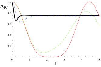
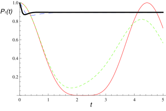
Figure 2: (Color online) The survival probability of the atomic state |1ket1\left|1\right\rangle as a function of time, for different values of the relevant parameters. (a) ωa/ωb=10subscript𝜔𝑎subscript𝜔𝑏10\omega_{a}/\omega_{b}=10, g12/ωb=g23/ωb=1subscript𝑔12subscript𝜔𝑏subscript𝑔23subscript𝜔𝑏1g_{12}/\omega_{b}=g_{23}/\omega_{b}=1, for different values of the temperature: T/ωb=0.1𝑇subscript𝜔𝑏0.1T/\omega_{b}=0.1 (red solid line), T/ωb=1𝑇subscript𝜔𝑏1T/\omega_{b}=1 (green dotted line), T/ωb=50𝑇subscript𝜔𝑏50T/\omega_{b}=50 (blue dashed line), T/ωb=250𝑇subscript𝜔𝑏250T/\omega_{b}=250 (black bold line). (b) ωa/ωb=50subscript𝜔𝑎subscript𝜔𝑏50\omega_{a}/\omega_{b}=50, g12/ωb=g23/ωb=1subscript𝑔12subscript𝜔𝑏subscript𝑔23subscript𝜔𝑏1g_{12}/\omega_{b}=g_{23}/\omega_{b}=1, for different values of the temperature: T/ωb=0.1𝑇subscript𝜔𝑏0.1T/\omega_{b}=0.1 (red solid line), T/ωb=1𝑇subscript𝜔𝑏1T/\omega_{b}=1 (green dotted line), T/ωb=250𝑇subscript𝜔𝑏250T/\omega_{b}=250 (blue dashed line), T/ωb=1250𝑇subscript𝜔𝑏1250T/\omega_{b}=1250 (black bold line).

In Fig. 2 are shown the evolutions of the survival probability for different temperatures and for different ratios of the frequencies of the two oscillators. It is evident that the higher the temperature the higher the survival probability at any time. Moreover, the smaller the ratio ωb/ωasubscript𝜔𝑏subscript𝜔𝑎\omega_{b}/\omega_{a} the higher the asymptotic value of P1(t)subscript𝑃1𝑡P_{1}(t).

It is worth noting the difference with the case analyzed in the previous paper on Zeno subspaces induced by temperature ref:MilitelloTQZE2011 . In fact, in that case the limit of the survival probability for T𝑇T\rightarrow\infty is unity, while in the present case the survival probability does not tend toward unity, unless assuming ωb/ωa0subscript𝜔𝑏subscript𝜔𝑎0\omega_{b}/\omega_{a}\rightarrow 0 (or |g12|/|g23|0subscript𝑔12subscript𝑔230|g_{12}|/|g_{23}|\rightarrow 0). This difference can be explained analyzing the physical mechanism on the basis of these Zeno-like behaviors induced by temperature. Indeed, the key points are two: first, in each invariant subspace the strength of the coupling with an oscillator grows up as the number of excitations increases; second, the higher the temperature the more the subspaces with high excitation numbers are populated. Now, in the case of Ref. ref:MilitelloTQZE2011 the interaction 12121-2 is not assisted by an harmonic oscillator and therefore it is not strengthened by temperature as the interaction 23232-3 is. As a consequence, an higher temperature makes the ratio between the two coupling strengths tend toward zero in most of the subspaces. On the contrary, in the present case, both couplings, 12121-2 and 23232-3, are effectively enhanced by temperature, and one needs ωbωamuch-less-thansubscript𝜔𝑏subscript𝜔𝑎\omega_{b}\ll\omega_{a} in order to make the coupling 23232-3 prevail in the majority of the subspaces. Indeed, ωbωamuch-less-thansubscript𝜔𝑏subscript𝜔𝑎\omega_{b}\ll\omega_{a} means that excited states of the oscillator b𝑏b are more populated than the corresponding states of oscillator a𝑎a, at the same temperature. If this condition (or the alternative one, i.e., |g12|/|g23|1much-less-thansubscript𝑔12subscript𝑔231|g_{12}|/|g_{23}|\ll 1) is not properly fulfilled, occurrence of Zeno dynamics is attenuated.

II.3 Low vs High Temperature

In order to better understand the role of temperature, it could be useful to compare the behaviors of the survival probability at low and high temperature.

In fact, in the zero-temperature case, the only block involved in the dynamics is the one related to na=nb=0subscript𝑛𝑎subscript𝑛𝑏0n_{a}=n_{b}=0, and the inhibition of the dynamics of |1,0,0ket100\left|1,0,0\right\rangle is determined by the condition |g23||g12|much-greater-thansubscript𝑔23subscript𝑔12|g_{23}|\gg|g_{12}|, so that it is essentially due to a significant difference between the strengths of the two couplings. On the contrary, when the high-temperature limit is considered, the parameter determining the minimum value of the survival probability is η𝜂\eta, as defined in Eq. (19), which involves both the coupling strengths and the frequencies of the oscillators. As already discussed before, a smaller frequency implies an higher degree of population of the excited levels of the oscillator, and eventually a stronger coupling in most of the Hilbert space.

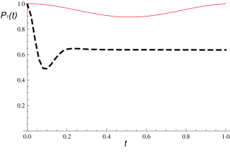
On this basis, one finds that Zeno dynamics is possible even in the case |g23|<|g12|subscript𝑔23subscript𝑔12|g_{23}|<|g_{12}|, provided ωbωamuch-less-thansubscript𝜔𝑏subscript𝜔𝑎\omega_{b}\ll\omega_{a} and temperature high enough. On the contrary, temperature can produce the opposite effect, determining disappearance of Zeno dynamics. As an example, consider the case |g23||g12|much-greater-thansubscript𝑔23subscript𝑔12|g_{23}|\gg|g_{12}|, which implies Zeno dynamics at zero temperature, and ωb>ωa|g23/g12|2ωasubscript𝜔𝑏subscript𝜔𝑎superscriptsubscript𝑔23subscript𝑔122much-greater-thansubscript𝜔𝑎\omega_{b}>\omega_{a}|g_{23}/g_{12}|^{2}\gg\omega_{a}, which renders η𝜂\eta large enough to invalidate inhibition of the dynamics. In Fig. 3 it is shown a case wherein by increasing temperature one lowers the survival probability at any time.
Refer to caption
Figure 3: (Color online) Survival probability of the atomic state |1ket1\left|1\right\rangle at low and high temperature. The relevant quantities are ωb/ωa=10subscript𝜔𝑏subscript𝜔𝑎10\omega_{b}/\omega_{a}=10, g12/ωa=1subscript𝑔12subscript𝜔𝑎1g_{12}/\omega_{a}=1, g23/g12=6subscript𝑔23subscript𝑔126g_{23}/g_{12}=6; temperature: T/ωa=0.1𝑇subscript𝜔𝑎0.1T/\omega_{a}=0.1 (red solid line), T/ωa=250𝑇subscript𝜔𝑎250T/\omega_{a}=250 (black dashed line).

III Detuning effects

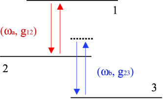
Let us now consider again the Hamiltonian in Eq.(LABEL:eq:complete_Hamiltonian_model) but without the resonance conditions (see Fig. 4). Generally speaking the presence of a detuning causes a diminishing of the interaction strength, so that the presence of a detuning in the 23232-3 transition will make us analyze the competition between detuning and temperature in connection with the occurrence of Zeno dynamics. On the contrary, the presence of a detuning in the 12121-2 transition would simply hinder the evolution of the initial atomic state (|1ket1\left|1\right\rangle) even in the absence of the second oscillator and relevant coupling. Therefore this analysis would be less interesting. Hence, for the sake of simplicity, let us assume that the transition 12121-2 is resonant with the relevant oscillator (ωa=ω1ω2subscript𝜔𝑎subscript𝜔1subscript𝜔2\omega_{a}=\omega_{1}-\omega_{2}), while the transition 23232-3 is assumed not to be resonant with the second oscillator: Δ=ωb(ω2ω3)0Δsubscript𝜔𝑏subscript𝜔2subscript𝜔30\Delta=\omega_{b}-(\omega_{2}-\omega_{3})\not=0. The restriction of the Hamiltonian in the generic invariant subspace corresponding to nasubscript𝑛𝑎n_{a} and nbsubscript𝑛𝑏n_{b} is given by the following matrix:

Hnanbsubscript𝐻subscript𝑛𝑎subscript𝑛𝑏\displaystyle H_{n_{a}n_{b}} =\displaystyle= (naωa+nbωb+ω1)𝕀3subscript𝑛𝑎subscript𝜔𝑎subscript𝑛𝑏subscript𝜔𝑏subscript𝜔1subscript𝕀3\displaystyle(n_{a}\omega_{a}+n_{b}\omega_{b}+\omega_{1})\mathbb{I}_{3} (24)
+\displaystyle\!\!\!\!\!\!+ (0g12na+10g12na+10g23nb+10g23nb+1Δ).0subscript𝑔12subscript𝑛𝑎10subscript𝑔12subscript𝑛𝑎10subscript𝑔23subscript𝑛𝑏10subscript𝑔23subscript𝑛𝑏1Δ\displaystyle\left(\begin{array}[]{ccc}0&g_{12}\sqrt{n_{a}+1}&0\cr\,\,g_{12}\sqrt{n_{a}+1}&0&\,\,g_{23}\sqrt{n_{b}+1}\cr 0&g_{23}\sqrt{n_{b}+1}&\Delta\end{array}\right)\,.
Refer to caption
Figure 4: (Color online) The upper atomic level (|1ket1\left|1\right\rangle) is resonantly coupled to the intermediate level (|2ket2\left|2\right\rangle), which in turn is non resonantly coupled to the lowest level (|3ket3\left|3\right\rangle).

According with the analysis in appendix A, in order to have inhibition of the dynamics of the state |1,na,nbket1subscript𝑛𝑎subscript𝑛𝑏\left|1,n_{a},n_{b}\right\rangle — making it a quasi-eigenstate of the Hamiltonian — one needs that g23nb+1subscript𝑔23subscript𝑛𝑏1g_{23}\sqrt{n_{b}+1} is much grater than g12na+1subscript𝑔12subscript𝑛𝑎1g_{12}\sqrt{n_{a}+1} and greater than ΔΔ\Delta. A large value of detuning can obstacle the appearance of Zeno dynamics, but larger values of temperature can establish again such a regime by populating more and more those subspaces wherein g23nb+1subscript𝑔23subscript𝑛𝑏1g_{23}\sqrt{n_{b}+1} is larger (and even much larger) than ΔΔ\Delta.

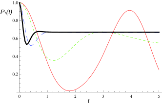
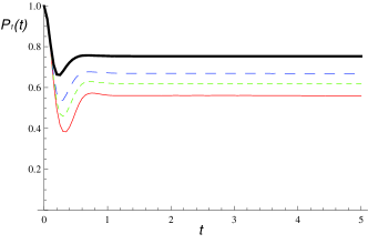
In Fig. 5 it is shown the behavior of the population of the atomic state |1ket1\left|1\right\rangle as a function of time but for different values of temperature and detuning. From Fig. 5a we learn that even in the presence of non vanishing detuning there is an increase of the survival probability when temperature becomes higher. Nevertheless, comparing the bold line in this figure with the one in Fig. 2a, we see that the asymptotic value of the population is slightly smaller in the presence of detuning, in spite of the fact that the temperature is the same.
Refer to caption
Refer to caption
Figure 5: (Color online) The survival probability of the atomic state |1ket1\left|1\right\rangle as a function of time, for different values of the relevant parameters. (a) ωa/ωb=10subscript𝜔𝑎subscript𝜔𝑏10\omega_{a}/\omega_{b}=10, g12/ωb=g23/ωb=1subscript𝑔12subscript𝜔𝑏subscript𝑔23subscript𝜔𝑏1g_{12}/\omega_{b}=g_{23}/\omega_{b}=1, Δ/ωb=1Δsubscript𝜔𝑏1\Delta/\omega_{b}=1, for different values of the temperature: T/ωb=0.1𝑇subscript𝜔𝑏0.1T/\omega_{b}=0.1 (red solid line), T/ωb=10𝑇subscript𝜔𝑏10T/\omega_{b}=10 (green dotted line), T/ωb=100𝑇subscript𝜔𝑏100T/\omega_{b}=100 (blue dashed line), T/ωb=250𝑇subscript𝜔𝑏250T/\omega_{b}=250 (black bold line). (b) ωa/ωb=10subscript𝜔𝑎subscript𝜔𝑏10\omega_{a}/\omega_{b}=10, g12/ωb=g23/ωb=1subscript𝑔12subscript𝜔𝑏subscript𝑔23subscript𝜔𝑏1g_{12}/\omega_{b}=g_{23}/\omega_{b}=1, kBT/ωb=250subscript𝑘𝐵𝑇subscript𝜔𝑏250k_{B}T/\omega_{b}=250, for different values of the detuning: Δ/ωb=4Δsubscript𝜔𝑏4\Delta/\omega_{b}=4 (red solid line), Δ/ωb=2Δsubscript𝜔𝑏2\Delta/\omega_{b}=2 (green dotted line), Δ/ωb=1Δsubscript𝜔𝑏1\Delta/\omega_{b}=1 (blue dashed line), Δ=0Δ0\Delta=0 (black bold line).

In Fig. 5b it is shown that, for a fixed value of temperature, a diminishing of the detuning produces an increase of the asymptotic population, as expected.

IV Attempt of Generalization

In view of a possible study of interactions between a few-level system and its environment, the previous analysis could deserve a generalization to the case wherein many harmonic oscillators couple both transitions, 12121-2 and 23232-3. Since we are interested to the case of quite different Bohr frequencies, we can consider two independent sets of oscillators. The relevant Hamiltonian is given by,

H^^𝐻\displaystyle\hat{H} =\displaystyle= kωn|nn|+k=1pνka^ka^k+l=1qμlb^lb^lsubscript𝑘subscript𝜔𝑛ket𝑛bra𝑛superscriptsubscript𝑘1𝑝subscript𝜈𝑘superscriptsubscript^𝑎𝑘subscript^𝑎𝑘superscriptsubscript𝑙1𝑞subscript𝜇𝑙superscriptsubscript^𝑏𝑙subscript^𝑏𝑙\displaystyle\sum_{k}\omega_{n}\left|n\right\rangle\left\langle n\right|+\sum_{k=1}^{p}\nu_{k}\hat{a}_{k}^{\dagger}\hat{a}_{k}+\sum_{l=1}^{q}\mu_{l}\hat{b}_{l}^{\dagger}\hat{b}_{l}
+\displaystyle+ k=1pgk(12)(|12|a^k+|21|a^k)superscriptsubscript𝑘1𝑝subscriptsuperscript𝑔12𝑘ket1quantum-operator-product2limit-fromsubscript^𝑎𝑘2bra1superscriptsubscript^𝑎𝑘\displaystyle\sum_{k=1}^{p}g^{(12)}_{k}(\left|1\right\rangle\left\langle 2\right|\hat{a}_{k}+\left|2\right\rangle\left\langle 1\right|\hat{a}_{k}^{\dagger})
+\displaystyle+ l=1qgl(23)(|23|b^l+|32|b^l),superscriptsubscript𝑙1𝑞subscriptsuperscript𝑔23𝑙ket2quantum-operator-product3limit-fromsubscript^𝑏𝑙3bra2superscriptsubscript^𝑏𝑙\displaystyle\sum_{l=1}^{q}g^{(23)}_{l}(\left|2\right\rangle\left\langle 3\right|\hat{b}_{l}+\left|3\right\rangle\left\langle 2\right|\hat{b}_{l}^{\dagger})\,,

which conserves the following quantity:

N^=2|11|+|22|+k=1pa^ka^k+l=1qb^lb^l.^𝑁2ket1bra1ket2bra2superscriptsubscript𝑘1𝑝superscriptsubscript^𝑎𝑘subscript^𝑎𝑘superscriptsubscript𝑙1𝑞superscriptsubscript^𝑏𝑙subscript^𝑏𝑙\displaystyle\hat{N}=2\left|1\right\rangle\left\langle 1\right|+\left|2\right\rangle\left\langle 2\right|+\sum_{k=1}^{p}\hat{a}_{k}^{\dagger}\hat{a}_{k}+\sum_{l=1}^{q}\hat{b}_{l}^{\dagger}\hat{b}_{l}\,. (27)

Therefore the Hilbert space is partitioned into invariant subspaces npmqsubscriptsubscript𝑛𝑝subscript𝑚𝑞{\cal H}_{\vec{n}_{p}\vec{m}_{q}} of dimension dimnpmq=1+p+pqdimensionsubscriptsubscript𝑛𝑝subscript𝑚𝑞1𝑝𝑝𝑞\dim{\cal H}_{\vec{n}_{p}\vec{m}_{q}}=1+p+pq and spanned by the following vectors: |1,np,mq|1,n1,np,m1,mqket1subscript𝑛𝑝subscript𝑚𝑞ket1subscript𝑛1subscript𝑛𝑝subscript𝑚1subscript𝑚𝑞\left|1,\vec{n}_{p},\vec{m}_{q}\right\rangle\equiv\left|1,n_{1},...n_{p},m_{1},...m_{q}\right\rangle;    (nk+1)1/2a^k|2,np,mqsuperscriptsubscript𝑛𝑘112superscriptsubscript^𝑎𝑘ket2subscript𝑛𝑝subscript𝑚𝑞(n_{k}+1)^{-1/2}\hat{a}_{k}^{\dagger}\left|2,\vec{n}_{p},\vec{m}_{q}\right\rangle with k=1,p𝑘1𝑝k=1,...p;    (nk+1)1/2(ml+1)1/2a^kb^l|3,np,mqsuperscriptsubscript𝑛𝑘112superscriptsubscript𝑚𝑙112superscriptsubscript^𝑎𝑘superscriptsubscript^𝑏𝑙ket3subscript𝑛𝑝subscript𝑚𝑞(n_{k}+1)^{-1/2}(m_{l}+1)^{-1/2}\hat{a}_{k}^{\dagger}\hat{b}_{l}^{\dagger}\left|3,\vec{n}_{p},\vec{m}_{q}\right\rangle, with k=1,p𝑘1𝑝k=1,...p and l=1,q𝑙1𝑞l=1,...q.

The restriction of the Hamiltonian to each subspace has the following structure:

Bp×q=(δ0α1α2αp0000000α1δ100β11β1q0000α20δ2000β21β2q00αp00δp0000βp1βpq0β1100δ110000000000β1q000δ1q000000β21000δ210000000000β2q0000δ2q00000βp10000δp1000000000βpq00000δpq),subscript𝐵𝑝𝑞subscript𝛿0subscript𝛼1subscript𝛼2subscript𝛼𝑝0000000subscript𝛼1subscript𝛿100subscript𝛽11subscript𝛽1𝑞0000subscript𝛼20subscript𝛿2000subscript𝛽21subscript𝛽2𝑞00missing-subexpressionmissing-subexpressionmissing-subexpressionmissing-subexpressionmissing-subexpressionmissing-subexpressionmissing-subexpressionmissing-subexpressionmissing-subexpressionmissing-subexpressionsubscript𝛼𝑝00missing-subexpressionsubscript𝛿𝑝0000subscript𝛽𝑝1subscript𝛽𝑝𝑞0subscript𝛽1100subscript𝛿11missing-subexpression00000missing-subexpression00000subscript𝛽1𝑞000subscript𝛿1𝑞000000subscript𝛽21000subscript𝛿21000missing-subexpressionmissing-subexpression0000000subscript𝛽2𝑞0000subscript𝛿2𝑞00missing-subexpressionmissing-subexpression000subscript𝛽𝑝10000subscript𝛿𝑝10missing-subexpressionmissing-subexpression00missing-subexpression000000subscript𝛽𝑝𝑞00000subscript𝛿𝑝𝑞B_{p\times q}=\left(\begin{array}[]{ccccccccccccccc}\delta_{0}&\alpha_{1}&\alpha_{2}&...&\alpha_{p}&0&0&0&0&...&0&...&0&...&0\cr\alpha_{1}&\delta_{1}&0&...&0&\beta_{11}&...&\beta_{1q}&0&...&0&...&0&...&0\cr\alpha_{2}&0&\delta_{2}&...&0&0&...&0&\beta_{21}&...&\beta_{2q}&...&0&...&0\cr\vdots&\vdots&\vdots&\ddots&&\vdots&&&&&&&&&\cr\alpha_{p}&0&0&&\delta_{p}&0&...&0&0&...&0&...&\beta_{p1}&...&\beta_{pq}\cr 0&\beta_{11}&0&...&0&\delta_{11}&&0&0&...&0&...&0&...&0\cr\vdots&\vdots&\vdots&&\vdots&...&\ddots&\vdots&0&...&0&...&0&...&0\cr 0&\beta_{1q}&0&...&0&0&...&\delta_{1q}&0&...&0&...&0&...&0\cr 0&0&\beta_{21}&...&0&0&...&0&\delta_{21}&...&0&...&0&...&0\cr\vdots&\vdots&\vdots&&\vdots&\vdots&&0&0&\ddots&0&...&0&...&0\cr 0&0&\beta_{2q}&...&0&0&...&0&0&...&\delta_{2q}&...&0&...&0\cr\vdots&\vdots&\vdots&&\vdots&\vdots&&\vdots&\vdots&...&\vdots&\ddots&\vdots&...&\vdots\cr 0&0&0&...&\beta_{p1}&0&...&0&0&...&0&...&\delta_{p1}&...&0\cr\vdots&\vdots&\vdots&&\vdots&\vdots&&0&0&&0&...&0&\ddots&0\cr 0&0&0&...&\beta_{pq}&0&...&0&0&...&0&...&0&...&\delta_{pq}\cr\end{array}\right)\,, (28)

where the only non vanishing terms in a line or column are between two symbols different from ‘ 00’  in that line or column. In spite of this fact, the matrix is rather involved and difficult to study.

In the very special case of p=1𝑝1p=1, such structure becomes quite simple:

B1×q=(δα000αδ1β1β2βM0β1δ11000β20δ1200βM00δ1M),subscript𝐵1𝑞𝛿𝛼000𝛼subscript𝛿1subscript𝛽1subscript𝛽2subscript𝛽𝑀0subscript𝛽1subscript𝛿11000subscript𝛽20subscript𝛿1200subscript𝛽𝑀00subscript𝛿1𝑀B_{1\times q}=\left(\begin{array}[]{cccccc}\delta&\alpha&0&0&...&0\cr\alpha&\delta_{1}&\beta_{1}&\beta_{2}&...&\beta_{M}\cr 0&\beta_{1}&\delta_{11}&0&...&0\cr 0&\beta_{2}&0&\delta_{12}&...&0\cr\vdots&\vdots&\vdots&\vdots&\ddots&\vdots\cr 0&\beta_{M}&0&0&...&\delta_{1M}\cr\end{array}\right)\,, (29)

where α=α1𝛼subscript𝛼1\alpha=\alpha_{1} and βl=β1lsubscript𝛽𝑙subscript𝛽1𝑙\beta_{l}=\beta_{1l}. In the generic subspace npmqsubscriptsubscript𝑛𝑝subscript𝑚𝑞{\cal H}_{\vec{n}_{p}\vec{m}_{q}} one has α=g1(12)(n1+1)1/2𝛼superscriptsubscript𝑔112superscriptsubscript𝑛1112\alpha=g_{1}^{(12)}(n_{1}+1)^{1/2} and βl=gl(23)(ml+1)1/2subscript𝛽𝑙superscriptsubscript𝑔𝑙23superscriptsubscript𝑚𝑙112\beta_{l}=g_{l}^{(23)}(m_{l}+1)^{1/2}.

The matrix in Eq. (29) has the same structure of the matrix analyzed in the Appendix B of Ref. ref:MilitelloTQZE2011 . On the basis of that analysis, we claim that when the system starts form |1,n1,mqket1subscript𝑛1subscript𝑚𝑞\left|1,n_{1},\vec{m}_{q}\right\rangle and (lβl2)1/2|α|much-greater-thansuperscriptsubscript𝑙superscriptsubscript𝛽𝑙212𝛼(\sum_{l}\beta_{l}^{2})^{1/2}\gg|\alpha| then the dynamics is hindered. Therefore, focusing our attention on the population of the atomic state |1ket1\left|1\right\rangle irrespectively of the number of excitations of the oscillators, by reasoning as in the previous sections, we can say that the evolution of such population turns out to be hindered when the frequencies μlsubscript𝜇𝑙\mu_{l} are smaller — preferably much smaller — than νν1𝜈subscript𝜈1\nu\equiv\nu_{1}. Such a condition on the frequencies makes the previous assertion true even if, for example, |g1(12)|2l|gl(23)|2similar-tosuperscriptsuperscriptsubscript𝑔1122subscript𝑙superscriptsuperscriptsubscript𝑔𝑙232|g_{1}^{(12)}|^{2}\sim\sum_{l}|g_{l}^{(23)}|^{2}.

V Discussion

The analysis developed in this paper shows in a clear way the role of the temperature in determining the occurrence of Zeno dynamics.

In particular, we have considered a few-level system prepared in an excited state and interacting with a set of harmonic oscillators initially prepared in thermal states at the same temperature. We have pointed out that an higher temperature implies a more significant role of the subspaces of the Hilbert space characterized by higher numbers of excitations, which in turn imply stronger effective couplings. The smaller the frequency of an oscillator the more its excited states are involved in the dynamics, for a given temperature. Therefore, the presence of a coupling between the lowest state |3ket3\left|3\right\rangle and the intermediate one |2ket2\left|2\right\rangle can significantly weaken the effects of the 12121-2 coupling, especially when the Bohr frequency of the 23232-3 transition is sufficiently small. This is a significant difference between high-temperature and low-temperature limit, since in the latter case the role of the frequencies is absent and only coupling strengths are important.

This analysis is the prosecution of the study developed in Ref. ref:MilitelloTQZE2011 where the 12121-2 coupling was induced by an external field assumed not to be affected by temperature. In the present work, instead, we have considered the competition between the growing of both the couplings, 12121-2 and 23232-3, and the role of temperature and Bohr frequencies in making one of them prevail.

A further analysis aimed at considering a set of harmonic oscillators driving each atomic transition — similar to the one performed in the previous paper — would be appropriate. Some preliminary results have been reported in section IV.

Another point that could deserve attention is the role of possible counter rotating terms in the interaction between the few-level system and the bosonic part of the total system.

VI Acknowledgements

The Author wishes to thank Antonino Messina and Matteo Scala for carefully reading the manuscript.

Appendix A

In this appendix we prove that a matrix of the following form (written in the basis |Aket𝐴\left|A\right\rangle, |Bket𝐵\left|B\right\rangle, |Cket𝐶\left|C\right\rangle):

M=(0α10α10α20α2Δ),𝑀0subscript𝛼10superscriptsubscript𝛼10subscript𝛼20superscriptsubscript𝛼2Δ\displaystyle M=\left(\begin{array}[]{ccc}0&\alpha_{1}&0\cr\alpha_{1}^{*}&0&\,\,\alpha_{2}\cr 0&\alpha_{2}^{*}&\Delta\end{array}\right)\,, (33)

has an eigenvalue whose corresponding eigenstate becomes closer to |Aket𝐴\left|A\right\rangle as the modulus of the coupling constant α2subscript𝛼2\alpha_{2} grows up.

Let us first consider the special situation Δ=0Δ0\Delta=0, in which case we can directly check that λ=0𝜆0\lambda=0 is an eigenvalue and that the corresponding eigenstate is

|0=α2α|Aα1α|C,α=|α1|2+|α2|2,formulae-sequenceket0subscript𝛼2𝛼ket𝐴superscriptsubscript𝛼1𝛼ket𝐶𝛼superscriptsubscript𝛼12superscriptsubscript𝛼22\left|0\right\rangle=\frac{\alpha_{2}}{\alpha}\left|A\right\rangle-\frac{\alpha_{1}^{*}}{\alpha}\left|C\right\rangle\,,\qquad\alpha=\sqrt{|\alpha_{1}|^{2}+|\alpha_{2}|^{2}}\,\,, (34)

from which one deduces that |A|0|=|α2/α|inner-product𝐴0subscript𝛼2𝛼|\left\langle A|0\right\rangle|=|\alpha_{2}/\alpha| tends toward unity in the limit |α1||α2|much-less-thansubscript𝛼1subscript𝛼2|\alpha_{1}|\ll|\alpha_{2}|.

Concerning the general case Δ0Δ0\Delta\not=0, the secular polynomial P(λ)=det(Mλ𝕀3)𝑃𝜆𝑀𝜆subscript𝕀3P(\lambda)=\det(M-\lambda\mathbb{I}_{3}) is:

P(λ)=λ3+Δλ2+(|α1|2+|α2|2)λ|α1|2Δ.𝑃𝜆superscript𝜆3Δsuperscript𝜆2superscriptsubscript𝛼12superscriptsubscript𝛼22𝜆superscriptsubscript𝛼12Δ\displaystyle P(\lambda)=-\lambda^{3}+\Delta\lambda^{2}+(|\alpha_{1}|^{2}+|\alpha_{2}|^{2})\lambda-|\alpha_{1}|^{2}\Delta\,. (35)

It turns out that

P(0)=|α1|2Δ,𝑃0superscriptsubscript𝛼12Δ\displaystyle P(0)=-|\alpha_{1}|^{2}\Delta\,, (36a)
and
P(|α12||α22|Δ)=|α1|4|α2|2Δ+(|α1α2|4|α1α2|6)Δ3,𝑃superscriptsubscript𝛼12superscriptsubscript𝛼22Δsuperscriptsubscript𝛼14superscriptsubscript𝛼22Δsuperscriptsubscript𝛼1subscript𝛼24superscriptsubscript𝛼1subscript𝛼26superscriptΔ3\displaystyle P\left(\frac{|\alpha_{1}^{2}|}{|\alpha_{2}^{2}|}\Delta\right)=\frac{|\alpha_{1}|^{4}}{|\alpha_{2}|^{2}}\Delta+\left(\left|\frac{\alpha_{1}}{\alpha_{2}}\right|^{4}-\left|\frac{\alpha_{1}}{\alpha_{2}}\right|^{6}\right)\Delta^{3}\,,

which for Δ0Δ0\Delta\not=0 and |α1|<|α2|subscript𝛼1subscript𝛼2|\alpha_{1}|<|\alpha_{2}| implies a change of sign. Therefore there is an eigenvalue η𝜂\eta of modulus |η|<|α12Δ/α22|𝜂superscriptsubscript𝛼12Δsuperscriptsubscript𝛼22|\eta|<|\alpha_{1}^{2}\Delta/\alpha_{2}^{2}|. The relevant eigenvector is:

|η=𝒫η(|A+ηα1|Bηα2(Δη)α1|C),ket𝜂subscript𝒫𝜂ket𝐴𝜂subscript𝛼1ket𝐵𝜂superscriptsubscript𝛼2Δ𝜂subscript𝛼1ket𝐶\displaystyle\left|\eta\right\rangle=\mathcal{P}_{\eta}\left(\left|A\right\rangle+\frac{\eta}{\alpha_{1}}\left|B\right\rangle-\frac{\eta\,\alpha_{2}^{*}}{(\Delta-\eta)\,\alpha_{1}}\left|C\right\rangle\right)\,, (37a)
with
𝒫η=[1+|η|2|α1|2+|η|2|α2|2|Δη|2|α1|2]1/2.subscript𝒫𝜂superscriptdelimited-[]1superscript𝜂2superscriptsubscript𝛼12superscript𝜂2superscriptsubscript𝛼22superscriptΔ𝜂2superscriptsubscript𝛼1212\displaystyle\mathcal{P}_{\eta}=\left[1+\frac{|\eta|^{2}}{|\alpha_{1}|^{2}}+\frac{|\eta|^{2}|\alpha_{2}|^{2}}{|\Delta-\eta|^{2}\,|\alpha_{1}|^{2}}\right]^{-1/2}\,. (37b)

Now, assume |Δ|<|α2|Δsubscript𝛼2|\Delta|<|\alpha_{2}| and |α1||α2|much-less-thansubscript𝛼1subscript𝛼2|\alpha_{1}|\ll|\alpha_{2}| (which in turn implies |η||Δ|much-less-than𝜂Δ|\eta|\ll|\Delta| and then |Δ/(Δη)|<2ΔΔ𝜂2|\Delta/(\Delta-\eta)|<2), one finds that |η/α1|<|α1/α2|×|Δ/α2|<|α1/α2|𝜂subscript𝛼1subscript𝛼1subscript𝛼2Δsubscript𝛼2subscript𝛼1subscript𝛼2|\eta/\alpha_{1}|<|\alpha_{1}/\alpha_{2}|\times|\Delta/\alpha_{2}|<|\alpha_{1}/\alpha_{2}| and |η2α22/[(Δη)2α12]|<|α1/α2|2×|Δ/(Δη)|2<2|α1/α2|2superscript𝜂2superscriptsubscript𝛼22delimited-[]superscriptΔ𝜂2superscriptsubscript𝛼12superscriptsubscript𝛼1subscript𝛼22superscriptΔΔ𝜂22superscriptsubscript𝛼1subscript𝛼22\left|\eta^{2}\alpha_{2}^{2}/[(\Delta-\eta)^{2}\,\alpha_{1}^{2}]\right|<|\alpha_{1}/\alpha_{2}|^{2}\times|\Delta/(\Delta-\eta)|^{2}<2|\alpha_{1}/\alpha_{2}|^{2}. Then, under the previous hypotheses one has |A|η|=𝒫η1inner-product𝐴𝜂subscript𝒫𝜂1|\left\langle A|\eta\right\rangle|=\mathcal{P}_{\eta}\rightarrow 1.

We conclude reminding that (see appendix A of Ref.ref:MilitelloTQZE2011 ) if the system is prepared in the initial state |ψ(0)=|Aket𝜓0ket𝐴\left|\psi(0)\right\rangle=\left|A\right\rangle, then the survival probability has a non vanishing lower bound: PA(t)=|A|ψ(t)|2(2|A|η|21)2subscript𝑃𝐴𝑡superscriptinner-product𝐴𝜓𝑡2superscript2superscriptinner-product𝐴𝜂212P_{A}(t)=|\left\langle A|\psi(t)\right\rangle|^{2}\geq(2|\left\langle A|\eta\right\rangle|^{2}-1)^{2}, which of course is close to unity when |A|η|1inner-product𝐴𝜂1|\left\langle A|\eta\right\rangle|\approx 1.

References

  • (1) B. Misra and E. C. G. Sudarshan, J. Math. Phys. 18, 7456 (1977).
  • (2) W. M. Itano, D. J. Heinzen, J. J. Bollinger and D. J. Wineland, Phys. Rev. A 41 2295 (1990).
  • (3) S. R. Wilkinson, C. F. Bharucha, M. C. Fischer, K. W. Madison, P. R. Morrow, Qian Niu, Bala Sundaram, and M. G. Raizen, Nature 387, 575 (1997).
  • (4) L. S. Schulman, Phys. Rev. A 57, 1509 (1998).
  • (5) A. D. Panov, Phys. Lett. A 260, 441 (1999).
  • (6) J. Audretsch, M. B. Mensky, A. D. Panov, Phys.Lett. A 261, 44 (1999).
  • (7) M. Scala, B. Militello, A. Messina, and N. V. Vitanov, Phys. Rev. A 81, 053847 (2010).
  • (8) B. Militello, M. Scala, A. Messina and N. V. Vitanov, Phys. Scr. T 143, 014019 (2011).
  • (9) P. Facchi and S. Pascazio, Progress in Optics 41 edited by E. Wolf, Elsevier, Amsterdam, 2001.
  • (10) B. Militello, A. Messina and A. Napoli, Phys. Lett. A 286, 369 (2001).
  • (11) B. Militello, A. Messina and A. Napoli, Fortscr. Phys. 49, 1041 (2001).
  • (12) P. Facchi and S. Pascazio, Phys. Rev. Lett. 89, 080401 (2002).
  • (13) P. Facchi, D. A. Lidar and S. Pascazio, Phys. Rev. A 69, 032314 (2004).
  • (14) P. Facchi and S. Pascazio, J. Phys. A: Math. Theor. 41, 493001 (2008).
  • (15) P. Facchi, G. Marmo and S. Pascazio, J. Phys.: Conf. Ser. 196, 012017 (2009).
  • (16) Keisuke Fujii and Katsuji Yamamoto, Phys. Rev. A 82, 042109 (2010).
  • (17) Gonzalo Alvarez, D. D. Bhaktavatsala Rao, L. Frydman, and G. Kurizki, Phys. Rev. Lett. 105, 160401 (2010).
  • (18) R. Schützhold and G. Gnanapragasam, Phys. Rev. A 82, 022120 (2010).
  • (19) D. Home and M. A. B. Whitaker, Ann. Phys. 258, 237 (1997).
  • (20) A. Peres, Am. J. Phys. 48, 931 (1980).
  • (21) J. Ruseckas, Phys. Rev. A 66, 012105 (2002).
  • (22) S. Maniscalco, J. Piilo and K.-A. Suominen, Phys. Rev. Lett. 97, 130402 (2006).
  • (23) M. Scala, B. Militello, A. Messina, N. V. Vitanov, Phys. Rev. A 84, 023416 (2011).
  • (24) B. Militello, M. Scala, A. Messina, Phys. Rev. A 84, 022106 (2011).