Adaptation and migration of a population between patches

Sepideh Mirrahimi CMAP, Ecole Polytechnique, CNRS, INRIA. Route de Saclay, 91128 Palaiseau Cedex, France. Email: mirrahimi@cmap.polytechnique.fr.
Abstract

A Hamilton-Jacobi formulation has been established previously for phenotypically structured population models where the solution concentrates as Dirac masses in the limit of small diffusion. Is it possible to extend this approach to spatial models? Are the limiting solutions still in the form of sums of Dirac masses? Does the presence of several habitats lead to polymorphic situations?

We study the stationary solutions of a structured population model, while the population is structured by continuous phenotypical traits and discrete positions in space. The growth term varies from one habitable zone to another, for instance because of a change in the temperature. The individuals can migrate from one zone to another with a constant rate. The mathematical modeling of this problem, considering mutations between phenotypical traits and competitive interaction of individuals within each zone via a single resource, leads to a system of coupled parabolic integro-differential equations. We study the asymptotic behavior of the stationary solutions to this model in the limit of small mutations. The limit, which is a sum of Dirac masses, can be described with the help of an effective Hamiltonian. The presence of migration can modify the dominant traits and lead to polymorphic situations.

Key-Words: Structured populations, phenotypical and spatial structure, Hamilton-Jacobi equation, viscosity solutions, Dirac concentrations, stationary solutions

AMS Class. No: 35B25, 47G20, 49L25, 92D15

1 Introduction

Non-local Lotka-Volterra equations arise in models of adaptive evolution of phenotypically structured populations. These equations have the property that the solutions concentrate generally, in the limit of small diffusion, on several isolated points, corresponding to distinct traits. Can we generalize these models by adding a spatial structure? How do the dominant traits evolve if we introduce a new habitat? To understand the interaction of ecological and evolutionary processes in population dynamics, spatial structure of the communities and adaptation of species to the environmental changes, it is crucial to dispose mathematical models that describe them jointly. We refer to [19] and the references therein for general literature on the subject. In this manuscript we consider a model where several distinct favorable habitable zones are possible. Population dynamics models structured by spatial patches have been studied using both deterministic and probabilistic methods (see for instance [30, 1]). Our model, in the case of two patches, is indeed very close to the one studied in [30] where the authors use adaptive dynamics theory (adaptive dynamics is a theory, based on dynamical systems and their stability, to study population dynamics [11]). Here we model similar phenomena, by adding a spatial structure to an earlier known integro-differential model describing the darwinian evolution. Integro-differential models have the advantage that the mutations can be considered directly in the model without assuming a separation of time scales of evolution and ecology. The present work provides a general description of the asymptotic stationary solutions, in the general case where two or several patches are possible.

We study the asymptotic behavior of solutions of a system of coupled elliptic integro-differential equations with small diffusion terms. These solutions are the stationary solutions to a parabolic system describing the dynamics of a population density. The individuals are characterized by phenotypical traits, that we denote by xd𝑥superscript𝑑x\in\mathbb{R}^{d}. They can move between two or several patches, which are favorable habitable zones, with constant rates (that we denote by ν1superscript𝜈1\nu^{1} and ν2superscript𝜈2\nu^{2} in the case of two patches). The mathematical modeling is based on the darwinian evolution and takes into account mutations and competition between the traits. There is a large literature for mathematical modeling and analysis on the subject of adaptive evolution, we refer the interested reader to [16, 15, 11, 12, 22, 10]. Here, we represent the birth and death term by a net growth term Ri(x,Ii)superscript𝑅𝑖𝑥superscript𝐼𝑖R^{i}(x,I^{i}) that is different in each patch, for instance because of a change in the temperature, and depends on the integral parameter Iisuperscript𝐼𝑖I^{i}, which corresponds to the the pressure exerted by the whole population within patch i𝑖i on the resource. To model the mutations, we use Laplace terms with a small rate ε𝜀\varepsilon that is introduced to consider only rare mutations. We study the asymptotic behavior of stationary solutions as the mutation rate ε𝜀\varepsilon goes to 00. The asymptotic solutions are generally concentrated on one or several Dirac masses. We describe the position and the weight of these Dirac masses using a Hamilton-Jacobi approach.

The time-dependent model, in the case of two patches, is written as

{tnε1εΔnε1=1εnε1R1(x,Iε1)+1εν2nε21εν1nε1,xd,tnε2εΔnε2=1εnε2R2(x,Iε2)+1εν1nε11εν2nε2,casessubscript𝑡superscriptsubscript𝑛𝜀1𝜀Δsuperscriptsubscript𝑛𝜀1absent1𝜀superscriptsubscript𝑛𝜀1superscript𝑅1𝑥superscriptsubscript𝐼𝜀11𝜀superscript𝜈2superscriptsubscript𝑛𝜀21𝜀superscript𝜈1superscriptsubscript𝑛𝜀1missing-subexpressionmissing-subexpressionmissing-subexpression𝑥superscript𝑑subscript𝑡superscriptsubscript𝑛𝜀2𝜀Δsuperscriptsubscript𝑛𝜀2absent1𝜀superscriptsubscript𝑛𝜀2superscript𝑅2𝑥superscriptsubscript𝐼𝜀21𝜀superscript𝜈1superscriptsubscript𝑛𝜀11𝜀superscript𝜈2superscriptsubscript𝑛𝜀2missing-subexpression\left\{\begin{array}[]{rlr}\partial_{t}n_{\varepsilon}^{1}-\varepsilon\Delta n_{\varepsilon}^{1}&=\frac{1}{\varepsilon}n_{\varepsilon}^{1}R^{1}(x,I_{\varepsilon}^{1})+\frac{1}{\varepsilon}\nu^{2}n_{\varepsilon}^{2}-\frac{1}{\varepsilon}\nu^{1}n_{\varepsilon}^{1},&\\ &&\quad x\in\mathbb{R}^{d},\\ \partial_{t}n_{\varepsilon}^{2}-\varepsilon\Delta n_{\varepsilon}^{2}&=\frac{1}{\varepsilon}n_{\varepsilon}^{2}R^{2}(x,I_{\varepsilon}^{2})+\frac{1}{\varepsilon}\nu^{1}n_{\varepsilon}^{1}-\frac{1}{\varepsilon}\nu^{2}n_{\varepsilon}^{2},&\end{array}\right. (1)

with

Iεi=ψi(x)nεi(x)𝑑x,for i=1,2.superscriptsubscript𝐼𝜀𝑖superscript𝜓𝑖𝑥superscriptsubscript𝑛𝜀𝑖𝑥differential-d𝑥for i=1,2.I_{\varepsilon}^{i}=\int\psi^{i}(x)n_{\varepsilon}^{i}(x)dx,\qquad\text{for $i=1,2.$} (2)

Such models, without the structure in space, have been derived from stochastic individual based models in the limit of large populations (see [7, 6]). This manuscript follows earlier works on parabolic Lotka-Volterra type equations to study concentration effects in models of phenotypically structured populations, that are based on a Hamilton-Jacobi formulation (see [12, 25, 2, 20]). The novelty of our work is that we add a spatial structure to the model by considering a finite number of favorable habitable zones. We thus have a system instead of a single equation. A Hamilton-Jacobi approach in the case of systems has also been introduced in [5] for an age structured model. See also [4] for a study of stationary solutions of the latter system. The Hamilton-Jacobi approach can also be used in problems other than adaptive evolution to prove concentration phenomena. See for instance [27, 26, 24] where related methods have been used to study the motion of motor proteins.

We are interested in the equilibria of 1 limited to a bounded domain, that are given by solutions of the following system

{ε2Δnε1=nε1R1(x,Iε1)+ν2nε2ν1nε1in BL(0),ε2Δnε2=nε2R2(x,Iε2)+ν1nε1ν2nε2in BL(0),nεin=0in BL(0) and for i=1, 2,casessuperscript𝜀2Δsuperscriptsubscript𝑛𝜀1absentsuperscriptsubscript𝑛𝜀1superscript𝑅1𝑥superscriptsubscript𝐼𝜀1superscript𝜈2superscriptsubscript𝑛𝜀2superscript𝜈1superscriptsubscript𝑛𝜀1in BL(0)missing-subexpressionmissing-subexpressionmissing-subexpressionsuperscript𝜀2Δsuperscriptsubscript𝑛𝜀2absentsuperscriptsubscript𝑛𝜀2superscript𝑅2𝑥superscriptsubscript𝐼𝜀2superscript𝜈1superscriptsubscript𝑛𝜀1superscript𝜈2superscriptsubscript𝑛𝜀2in BL(0)missing-subexpressionmissing-subexpressionmissing-subexpressionsuperscriptsubscript𝑛𝜀𝑖𝑛absent0in BL(0) and for i=1, 2\left\{\begin{array}[]{rll}-\varepsilon^{2}\Delta n_{\varepsilon}^{1}&=n_{\varepsilon}^{1}R^{1}(x,I_{\varepsilon}^{1})+\nu^{2}n_{\varepsilon}^{2}-\nu^{1}n_{\varepsilon}^{1}&\quad\text{in $B_{L}(0)$},\\ \\ -\varepsilon^{2}\Delta n_{\varepsilon}^{2}&=n_{\varepsilon}^{2}R^{2}(x,I_{\varepsilon}^{2})+\nu^{1}n_{\varepsilon}^{1}-\nu^{2}n_{\varepsilon}^{2}&\quad\text{in $B_{L}(0)$},\\ \\ \nabla n_{\varepsilon}^{i}\cdot\vec{n}&=0&\quad\text{in $\partial B_{L}(0)$ and for $i=1,\,2$},\end{array}\right. (3)

where BL(p)subscript𝐵𝐿𝑝B_{L}(p) is a ball of radius L𝐿L with center in p𝑝p and n(x)𝑛𝑥\vec{n}(x) is the unit normal vector, at the point xBL(0)𝑥subscript𝐵𝐿0x\in\partial B_{L}(0), to the boundary of BL(0)subscript𝐵𝐿0B_{L}(0). The Neumann boundary condition is a way to express that mutants cannot be born in dBL(0)superscript𝑑subscript𝐵𝐿0\mathbb{R}^{d}\setminus B_{L}(0).

To formulate our results we introduce the assumptions we will be using throughout the paper. We assume that, there exist positive constants amsubscript𝑎𝑚a_{m} and aMsubscript𝑎𝑀a_{M} such that

ψ1=ψ2=ψ,amψ(x)aM,ψ(x)W2,Aandψn=0 in BL(0).formulae-sequencesuperscript𝜓1superscript𝜓2𝜓subscript𝑎𝑚𝜓𝑥subscript𝑎𝑀formulae-sequencesubscriptnorm𝜓𝑥superscript𝑊2𝐴and𝜓𝑛0 in BL(0)\psi^{1}=\psi^{2}=\psi,\quad a_{m}\leq\psi(x)\leq a_{M},\quad\|\psi(x)\|_{W^{2,\infty}}\leq A\quad\text{and}\quad\nabla\psi\cdot\vec{n}=0\text{ in $\partial B_{L}(0)$}. (4)

Moreover there exist positive constants Imsubscript𝐼𝑚I_{m}, IMsubscript𝐼𝑀I_{M}, δ𝛿\delta and C𝐶C such that, for all xBL(0)𝑥subscript𝐵𝐿0x\in B_{L}(0) and i,j=1, 2formulae-sequence𝑖𝑗12i,j=1,\,2,

δmin(Ri(x,νjνiIm),Ri(x,Im)),max(Ri(x,νjνiIM),Ri(x,IM))δ,formulae-sequence𝛿superscript𝑅𝑖𝑥superscript𝜈𝑗superscript𝜈𝑖subscript𝐼𝑚superscript𝑅𝑖𝑥subscript𝐼𝑚superscript𝑅𝑖𝑥superscript𝜈𝑗superscript𝜈𝑖subscript𝐼𝑀superscript𝑅𝑖𝑥subscript𝐼𝑀𝛿\delta\leq\min\left(R^{i}(x,\frac{\nu^{j}}{\nu^{i}}I_{m}),R^{i}(x,I_{m})\right),\quad\max\left(R^{i}(x,\frac{\nu^{j}}{\nu^{i}}I_{M}),R^{i}(x,I_{M})\right)\leq-\delta, (5)
CRiI(x,I)1C,𝐶superscript𝑅𝑖𝐼𝑥𝐼1𝐶-C\leq\frac{\partial R^{i}}{\partial I}(x,I)\leq-\frac{1}{C}, (6)
DRξξi(x,I),for xBL(0)I[Im,IM]ξd|ξ|=1 and i=1,2.𝐷superscriptsubscript𝑅𝜉𝜉𝑖𝑥𝐼for xBL(0)I[Im,IM]ξd|ξ|=1 and i=1,2.-D\leq R_{\xi\xi}^{i}(x,I),\quad\text{for $x\in B_{L}(0)$, $I\in[I_{m},I_{M}]$, $\xi\in\mathbb{R}^{d}$, $|\xi|=1$ and $i=1,2$.} (7)

We use the Hopf-Cole transformation

nεi=exp(uεiε),for i=1,2,superscriptsubscript𝑛𝜀𝑖superscriptsubscript𝑢𝜀𝑖𝜀for i=1,2,n_{\varepsilon}^{i}=\exp(\frac{u_{\varepsilon}^{i}}{\varepsilon}),\qquad\text{for $i=1,2,$} (8)

and replace the latter in the system satisfied by nεisuperscriptsubscript𝑛𝜀𝑖n_{\varepsilon}^{i} to obtain

{εΔuε1=|uε1|2+R1(x,Iε1)+ν2exp(uε2uε1ε)ν1,in BL(0),εΔuε2=|uε2|2+R2(x,Iε2)+ν1exp(uε1uε2ε)ν2in BL(0),uεin=0in BL(0)and for i=1, 2.cases𝜀Δsuperscriptsubscript𝑢𝜀1absentsuperscriptsuperscriptsubscript𝑢𝜀12superscript𝑅1𝑥superscriptsubscript𝐼𝜀1superscript𝜈2superscriptsubscript𝑢𝜀2superscriptsubscript𝑢𝜀1𝜀superscript𝜈1in BL(0)missing-subexpressionmissing-subexpressionmissing-subexpression𝜀Δsuperscriptsubscript𝑢𝜀2absentsuperscriptsuperscriptsubscript𝑢𝜀22superscript𝑅2𝑥superscriptsubscript𝐼𝜀2superscript𝜈1superscriptsubscript𝑢𝜀1superscriptsubscript𝑢𝜀2𝜀superscript𝜈2in BL(0)missing-subexpressionmissing-subexpressionmissing-subexpressionsuperscriptsubscript𝑢𝜀𝑖𝑛absent0in BL(0)missing-subexpressionmissing-subexpressionand for i=1, 2\left\{\begin{array}[]{rll}-\varepsilon\Delta u_{\varepsilon}^{1}&=|\nabla u_{\varepsilon}^{1}|^{2}+R^{1}(x,I_{\varepsilon}^{1})+\nu^{2}\exp(\frac{u_{\varepsilon}^{2}-u_{\varepsilon}^{1}}{\varepsilon})-\nu^{1},&\quad\text{in $B_{L}(0)$},\\ \\ -\varepsilon\Delta u_{\varepsilon}^{2}&=|\nabla u_{\varepsilon}^{2}|^{2}+R^{2}(x,I_{\varepsilon}^{2})+\nu^{1}\exp(\frac{u_{\varepsilon}^{1}-u_{\varepsilon}^{2}}{\varepsilon})-\nu^{2}&\quad\text{in $B_{L}(0)$},\\ \\ \nabla u_{\varepsilon}^{i}\cdot\vec{n}&=0&\quad\text{in $\partial B_{L}(0)$}\\ &&\text{and for $i=1,\,2$}.\end{array}\right. (9)

We prove the following

Theorem 1.1

Assume 46. Then, as ε0𝜀0\varepsilon\to 0 along subsequences, both sequences (uε1)εsubscriptsuperscriptsubscript𝑢𝜀1𝜀(u_{\varepsilon}^{1})_{\varepsilon} and (uε2)εsubscriptsuperscriptsubscript𝑢𝜀2𝜀(u_{\varepsilon}^{2})_{\varepsilon} converge uniformly in BL(0)subscript𝐵𝐿0B_{L}(0) to a continuous function uC(BL(0))𝑢Csubscript𝐵𝐿0u\in\mathrm{C}(B_{L}(0)) and (Iε1,Iε2)superscriptsubscript𝐼𝜀1superscriptsubscript𝐼𝜀2(I_{\varepsilon}^{1},I_{\varepsilon}^{2}) goes to (I1,I2)superscript𝐼1superscript𝐼2(I^{1},I^{2}), with (u,I1,I2)𝑢superscript𝐼1superscript𝐼2(u,I^{1},I^{2}) such that u𝑢u is a viscosity solution to the following equation

{|u|2=H(x,I1,I2),in BL(0),maxxBL(0)u(x)=0,casessuperscript𝑢2𝐻𝑥superscript𝐼1superscript𝐼2in BL(0)missing-subexpressionmissing-subexpressionsubscript𝑥subscript𝐵𝐿0𝑢𝑥0missing-subexpression\left\{\begin{array}[]{ll}-|\nabla u|^{2}=H(x,I^{1},I^{2}),&\quad\text{in $B_{L}(0)$},\\ \\ \max_{x\in B_{L}(0)}u(x)=0,\end{array}\right. (10)

with

H(x,I1,I2) the largest eigenvalue of the matrix𝒜=(R1(x,I1)ν1ν2ν1R2(x,I2)ν2).H(x,I1,I2) the largest eigenvalue of the matrix𝒜superscript𝑅1𝑥superscript𝐼1superscript𝜈1superscript𝜈2superscript𝜈1superscript𝑅2𝑥superscript𝐼2superscript𝜈2\begin{array}[]{c}\text{$H(x,I^{1},I^{2})$ the largest eigenvalue of the matrix}\\ \displaystyle\mathcal{A}=\left(\begin{array}[]{cc}R^{1}(x,I^{1})-\nu^{1}&\nu^{2}\\ \nu^{1}&R^{2}(x,I^{2})-\nu^{2}\end{array}\right).\end{array} (11)

The function H𝐻H is indeed an effective Hamiltonian that contains information from the two patches and helps us in Theorem 1.2 to describe the support of the weak limits of (nε1,nε2)superscriptsubscript𝑛𝜀1superscriptsubscript𝑛𝜀2(n_{\varepsilon}^{1},n_{\varepsilon}^{2}) as ε0𝜀0\varepsilon\to 0. We can interpret H(x,I1,I2)𝐻𝑥superscript𝐼1superscript𝐼2H(x,I^{1},I^{2}) as the fitness of the system in the limit of ε0𝜀0\varepsilon\to 0 (see [23] for the definition of fitness).

The difficulty here is to find appropriate regularity estimates on uεisuperscriptsubscript𝑢𝜀𝑖u_{\varepsilon}^{i}, that we obtain using the Harnack inequality [3] and the Bernstein method [9]. To prove convergence to the Hamilton-Jacobi equation, we are inspired from the method of perturbed test functions in homogenization [14].

The above information on the limit of uεisuperscriptsubscript𝑢𝜀𝑖u_{\varepsilon}^{i} allows us to describe the limit of the densities nεisuperscriptsubscript𝑛𝜀𝑖n_{\varepsilon}^{i} as ε𝜀\varepsilon vanishes. We prove

Theorem 1.2

Assume 47. Consider a subsequence such that uε1superscriptsubscript𝑢𝜀1u_{\varepsilon}^{1} and uε2superscriptsubscript𝑢𝜀2u_{\varepsilon}^{2} converge uniformly to uC(BL(0))𝑢𝐶subscript𝐵𝐿0u\in C\left(B_{L}(0)\right) and (Iε1,Iε2)superscriptsubscript𝐼𝜀1superscriptsubscript𝐼𝜀2(I_{\varepsilon}^{1},I_{\varepsilon}^{2}) goes to (I1,I2)superscript𝐼1superscript𝐼2(I^{1},I^{2}), as ε0𝜀0\varepsilon\to 0, with (u,I1,I2)𝑢superscript𝐼1superscript𝐼2(u,I^{1},I^{2}) solution of 10. Let nεisuperscriptsubscript𝑛𝜀𝑖n_{\varepsilon}^{i}, for i=1,2𝑖12i=1,2, converge weakly in the sense of measures to nisuperscript𝑛𝑖n^{i} along this subsequence. We have

suppniΩΓ,for i=1,2,suppsuperscript𝑛𝑖ΩΓfor i=1,2,\mathrm{supp}\;n^{i}\subset\Omega\cap\Gamma,\quad\text{for $i=1,2$,} (12)

with

Ω={xBL(0)|u(x)=0},Γ={xBL(0)|H(x,I1,I2)=maxxBL(0)H(x,I1,I2)=0}.Ωconditional-set𝑥subscript𝐵𝐿0𝑢𝑥0Γconditional-set𝑥subscript𝐵𝐿0𝐻𝑥superscript𝐼1superscript𝐼2subscript𝑥subscript𝐵𝐿0𝐻𝑥superscript𝐼1superscript𝐼20\begin{array}[]{c}\Omega=\{x\in B_{L}(0)\,|\,u(x)=0\},\\ \Gamma=\{x\in B_{L}(0)\,|\,H(x,I^{1},I^{2})=\max_{x\in B_{L}(0)}H(x,I^{1},I^{2})=0\}.\end{array} (13)

Moreover, we have

(R1(x)ν1)n1(x)+ν2n2(x)=0,(R2(x)ν2)n2(x)+ν1n1(x)=0,in BL(0)formulae-sequencesuperscript𝑅1𝑥superscript𝜈1superscript𝑛1𝑥superscript𝜈2superscript𝑛2𝑥0superscript𝑅2𝑥superscript𝜈2superscript𝑛2𝑥superscript𝜈1superscript𝑛1𝑥0in subscript𝐵𝐿0\left(R^{1}(x)-\nu^{1}\right)n^{1}(x)+\nu^{2}n^{2}(x)=0,\quad\left(R^{2}(x)-\nu^{2}\right)n^{2}(x)+\nu^{1}n^{1}(x)=0,\quad\text{in }B_{L}(0) (14)

in the sense of distributions. The above condition is coupled by

BL(0)ψi(x)ni(x)=Ii.subscriptsubscript𝐵𝐿0superscript𝜓𝑖𝑥superscript𝑛𝑖𝑥superscript𝐼𝑖\int_{B_{L}(0)}\psi^{i}(x)n^{i}(x)=I^{i}. (15)

Theorem 1.2 provides us with a set of algebraic constraints on the limit, which allows us to describe the latter. In particular, if the support of nisuperscript𝑛𝑖n^{i}, for i=1,2𝑖12i=1,2, is a set of distinct points: suppni{x1,x2,,xk}suppsuperscript𝑛𝑖subscript𝑥1subscript𝑥2subscript𝑥𝑘\mathrm{supp}\,n^{i}\subset\{x_{1},x_{2},\cdots,x_{k}\}, 14 implies that

ni=j=1kρjiδ(xxj),for i=1,2,superscript𝑛𝑖superscriptsubscript𝑗1𝑘subscriptsuperscript𝜌𝑖𝑗𝛿𝑥subscript𝑥𝑗for i=1,2,n^{i}=\sum_{j=1}^{k}\rho^{i}_{j}\delta(x-x_{j}),\qquad\text{for $i=1,2$,} (16)

with

ρj2=ρj1(ν1R1(xj,I1)ν2)=ρj1(ν1ν2R2(xj,I2)).superscriptsubscript𝜌𝑗2superscriptsubscript𝜌𝑗1superscript𝜈1superscript𝑅1subscript𝑥𝑗superscript𝐼1superscript𝜈2superscriptsubscript𝜌𝑗1superscript𝜈1superscript𝜈2superscript𝑅2subscript𝑥𝑗superscript𝐼2\rho_{j}^{2}=\rho_{j}^{1}\left(\frac{\nu^{1}-R^{1}(x_{j},I^{1})}{\nu^{2}}\right)=\rho_{j}^{1}\left(\frac{\nu^{1}}{\nu^{2}-R^{2}(x_{j},I^{2})}\right). (17)

Furthermore, the weights (ρ1i,,ρki)subscriptsuperscript𝜌𝑖1subscriptsuperscript𝜌𝑖𝑘(\rho^{i}_{1},\cdots,\rho^{i}_{k}) satisfy the normalization condition

j=1kψi(xj)ρji=Ii,for i=1,2.superscriptsubscript𝑗1𝑘superscript𝜓𝑖subscript𝑥𝑗subscriptsuperscript𝜌𝑖𝑗superscript𝐼𝑖for i=1,2.\sum_{j=1}^{k}\psi^{i}(x_{j})\rho^{i}_{j}=I^{i},\qquad\ \text{for $i=1,2$.} (18)

Condition 17 means that the vector (ρj1ρj2)superscriptsubscript𝜌𝑗1superscriptsubscript𝜌𝑗2\left(\begin{array}[]{c}\rho_{j}^{1}\\ \rho_{j}^{2}\end{array}\right) is the eigenvector corresponding to the largest eigenvalue of the matrix 𝒜𝒜\mathcal{A} at the point xjsubscript𝑥𝑗x_{j}, which is 00. Thereby 17 implies once again that suppniΓsuppsuperscript𝑛𝑖Γ\mathrm{supp}\,n^{i}\subset\Gamma.

We point out that since nisuperscript𝑛𝑖n^{i}, for i=1,2𝑖12i=1,2, is such that the fitness H𝐻H vanishes on the support of nisuperscript𝑛𝑖n^{i} and is negative outside the support, we can interpret nisuperscript𝑛𝑖n^{i} as evolutionary stable distribution of the model. In adaptive dynamics, evolutionary stable distribution (ESD) corresponds to a distribution that remains stable after introduction of small mutants (see [21, 13, 17] for a more detailed definition). See also [10, 28] for related works on stability and convergence to ESD for trait-structured integro-differential models.

The set of assumptions in Theorem 1.2 allows us to describe the asymptotics of the stationary solutions, in the limit of rare or small mutations. In Section 5 we provide some examples where based on this information we can describe the asymptotics. In particular, we notice that the introduction of a new environment can lead to dimorphic situations. We refer to [8] for a related work using the Hamilton-Jacobi approach, where polymorphic situations can also appear in a model with multiple resources.

The paper is organized as follows. In Section 2 we prove some bounds on Iεsubscript𝐼𝜀I_{\varepsilon} and some regularity properties on uεsubscript𝑢𝜀u_{\varepsilon} that allow us to pass to the limit as ε0𝜀0\varepsilon\to 0 and derive the Hamilton-Jacobi equation with constraint. Theorem 1.1 is proved in Section 3. Using the results obtained on the asymptotic behavior of (uεi)εsubscriptsuperscriptsubscript𝑢𝜀𝑖𝜀(u_{\varepsilon}^{i})_{\varepsilon} we prove Theorem 1.2 in Section 4. In Section 5 we provide some examples where the information given by Theorem 1.1 and Theorem 1.2 allows us to describe the limit. The asymptotic behavior of the stationary solutions in a more general framework, where more than two habitable zones are considered, is given in Section 6. Finally in Section 7 we present some numerical simulations for the time-dependent problem and compare them with the behavior of stationary solutions.

2 Regularity results

Lemma 2.1

Under assumptions 46 we have, for εε0𝜀subscript𝜀0\varepsilon\leq\varepsilon_{0} chosen small enough,

ImIεiIM,for i=1, 2.formulae-sequencesubscript𝐼𝑚superscriptsubscript𝐼𝜀𝑖subscript𝐼𝑀for i=1, 2I_{m}\leq I_{\varepsilon}^{i}\leq I_{M},\qquad\text{for $i=1,\,2$}. (19)

In particular, along subsequences, (Iε1,Iε2)εsubscriptsuperscriptsubscript𝐼𝜀1superscriptsubscript𝐼𝜀2𝜀(I_{\varepsilon}^{1},I_{\varepsilon}^{2})_{\varepsilon} converges to (I1,I2)superscript𝐼1superscript𝐼2(I^{1},I^{2}), with ImI1,I2IMformulae-sequencesubscript𝐼𝑚superscript𝐼1superscript𝐼2subscript𝐼𝑀I_{m}\leq I^{1},\;I^{2}\leq I_{M}.

Remark 1

This is the only part, where we use Assumption 4. If (nε1,nε2)superscriptsubscript𝑛𝜀1superscriptsubscript𝑛𝜀2(n_{\varepsilon}^{1},n_{\varepsilon}^{2}) is a solution of 3 such that 19 is satisfied, then the results of Theorems 1.1 and 1.2 hold true without necessarily assuming 4. In particular, one can take ψ1ψ2not-equivalent-tosuperscript𝜓1superscript𝜓2\psi^{1}\not\equiv\psi^{2}.

Proof 1

We prove the result by contradiction. We suppose that Iε1>IMsuperscriptsubscript𝐼𝜀1subscript𝐼𝑀I_{\varepsilon}^{1}>I_{M} (the case with Iε2>IMsuperscriptsubscript𝐼𝜀2subscript𝐼𝑀I_{\varepsilon}^{2}>I_{M}, and the inequalities from below can be treated following similar arguments). We multiply the first equation in 3 by ψ(x)𝜓𝑥\psi(x), integrate, and use 4 to obtain

ε2AamIε1ψ(x)nε1(x)R1(x,Iε1)𝑑x+ν2Iε2ν1Iε1.superscript𝜀2𝐴subscript𝑎𝑚superscriptsubscript𝐼𝜀1𝜓𝑥superscriptsubscript𝑛𝜀1𝑥superscript𝑅1𝑥superscriptsubscript𝐼𝜀1differential-d𝑥superscript𝜈2superscriptsubscript𝐼𝜀2superscript𝜈1superscriptsubscript𝐼𝜀1-\varepsilon^{2}\frac{A}{a_{m}}I_{\varepsilon}^{1}\leq\int\psi(x)n_{\varepsilon}^{1}(x)R^{1}(x,I_{\varepsilon}^{1})dx+\nu^{2}I_{\varepsilon}^{2}-\nu^{1}I_{\varepsilon}^{1}.

Using now 5, 6 and the fact that Iε1>IMsuperscriptsubscript𝐼𝜀1subscript𝐼𝑀I_{\varepsilon}^{1}>I_{M} we deduce that, for εε0𝜀subscript𝜀0\varepsilon\leq\varepsilon_{0} small enough,

0(δε2Aam)Iε1ν2Iε2ν1Iε1,0𝛿superscript𝜀2𝐴subscript𝑎𝑚superscriptsubscript𝐼𝜀1superscript𝜈2superscriptsubscript𝐼𝜀2superscript𝜈1superscriptsubscript𝐼𝜀10\leq\left(\delta-\varepsilon^{2}\frac{A}{a_{m}}\right)I_{\varepsilon}^{1}\leq\nu^{2}I_{\varepsilon}^{2}-\nu^{1}I_{\varepsilon}^{1},

and thus

ν1ν2IMIε2.superscript𝜈1superscript𝜈2subscript𝐼𝑀superscriptsubscript𝐼𝜀2\frac{\nu^{1}}{\nu^{2}}\,I_{M}\leq I_{\varepsilon}^{2}.

Now we multiply the equations in 3 by ψ(x)𝜓𝑥\psi(x), integrate and add them and use 4 to obtain

ε2Aam(Iε1+Iε2)ψ(x)nε1(x)R1(x,Iε1)𝑑x+ψ(x)nε2(x)R2(x,Iε2)𝑑x.superscript𝜀2𝐴subscript𝑎𝑚superscriptsubscript𝐼𝜀1superscriptsubscript𝐼𝜀2𝜓𝑥superscriptsubscript𝑛𝜀1𝑥superscript𝑅1𝑥superscriptsubscript𝐼𝜀1differential-d𝑥𝜓𝑥superscriptsubscript𝑛𝜀2𝑥superscript𝑅2𝑥superscriptsubscript𝐼𝜀2differential-d𝑥-\varepsilon^{2}\frac{A}{a_{m}}(I_{\varepsilon}^{1}+I_{\varepsilon}^{2})\leq\int\psi(x)n_{\varepsilon}^{1}(x)R^{1}(x,I_{\varepsilon}^{1})dx+\int\psi(x)n_{\varepsilon}^{2}(x)R^{2}(x,I_{\varepsilon}^{2})dx.

From 5, 6 and the above bounds on Iε1superscriptsubscript𝐼𝜀1I_{\varepsilon}^{1} and Iε2superscriptsubscript𝐼𝜀2I_{\varepsilon}^{2} it follows that

ε2Aam(Iε1+Iε2)δ(Iε1+Iε2),superscript𝜀2𝐴subscript𝑎𝑚superscriptsubscript𝐼𝜀1superscriptsubscript𝐼𝜀2𝛿superscriptsubscript𝐼𝜀1superscriptsubscript𝐼𝜀2-\varepsilon^{2}\frac{A}{a_{m}}(I_{\varepsilon}^{1}+I_{\varepsilon}^{2})\leq-\delta(I_{\varepsilon}^{1}+I_{\varepsilon}^{2}),

which is not possible if ε𝜀\varepsilon is small enough. We conclude that Iε1IMsuperscriptsubscript𝐼𝜀1subscript𝐼𝑀I_{\varepsilon}^{1}\leq I_{M}.

Theorem 2.2

Assume 46. Then
(i) there exists a positive constant D𝐷D, such that for εε0𝜀subscript𝜀0\varepsilon\leq\varepsilon_{0},

|uεi(x)uεj(y)|Dε,for all x,yBL(0)|xy|ε and i,j{1,2}.superscriptsubscript𝑢𝜀𝑖𝑥superscriptsubscript𝑢𝜀𝑗𝑦𝐷𝜀for all x,yBL(0)|xy|ε and i,j{1,2}.|u_{\varepsilon}^{i}(x)-u_{\varepsilon}^{j}(y)|\leq D\varepsilon,\qquad\text{for all $x,\,y\in B_{L}(0)$, $|x-y|\leq\varepsilon$ and $i,\,j\in\{1,2\}$.} (20)

(ii) For i=1, 2𝑖12i=1,\,2 and all εε0𝜀subscript𝜀0\varepsilon\leq\varepsilon_{0}, the family (uε)εsubscriptsubscript𝑢𝜀𝜀(u_{\varepsilon})_{\varepsilon} is uniformly Lipschitz and uniformly bounded from below.
(iii) For all a>0𝑎0a>0, there exists ε1=ε1(a)subscript𝜀1subscript𝜀1𝑎\varepsilon_{1}=\varepsilon_{1}(a) such that for all εε1𝜀subscript𝜀1\varepsilon\leq\varepsilon_{1},

uεi(x)a,for xBL(0) and i=1, 2.superscriptsubscript𝑢𝜀𝑖𝑥𝑎for xBL(0) and i=1, 2.u_{\varepsilon}^{i}(x)\leq a,\qquad\text{for $x\in B_{L}(0)$ and $i=1,\,2$.} (21)
Proof 2

(i) We define

n~εi(y)=nεi(εy),for i=1, 2.superscriptsubscript~𝑛𝜀𝑖𝑦superscriptsubscript𝑛𝜀𝑖𝜀𝑦for i=1, 2.\widetilde{n}_{\varepsilon}^{i}(y)=n_{\varepsilon}^{i}(\varepsilon y),\qquad\text{for $i=1,\,2$.}

From 3 we have

{Δn~ε1=n~ε1R1(εx,Iε1)+ν2n~ε2ν1n~ε1in BLε(0),Δn~ε2=n~ε2R2(εx,Iε2)+ν1n~ε1ν2n~ε2in BLε(0),casesΔsuperscriptsubscript~𝑛𝜀1absentsuperscriptsubscript~𝑛𝜀1superscript𝑅1𝜀𝑥superscriptsubscript𝐼𝜀1superscript𝜈2superscriptsubscript~𝑛𝜀2superscript𝜈1superscriptsubscript~𝑛𝜀1in BLε(0)missing-subexpressionmissing-subexpressionmissing-subexpressionΔsuperscriptsubscript~𝑛𝜀2absentsuperscriptsubscript~𝑛𝜀2superscript𝑅2𝜀𝑥superscriptsubscript𝐼𝜀2superscript𝜈1superscriptsubscript~𝑛𝜀1superscript𝜈2superscriptsubscript~𝑛𝜀2in BLε(0)\displaystyle\left\{\begin{array}[]{rll}-\Delta\widetilde{n}_{\varepsilon}^{1}&=\widetilde{n}_{\varepsilon}^{1}R^{1}(\varepsilon x,I_{\varepsilon}^{1})+\nu^{2}\widetilde{n}_{\varepsilon}^{2}-\nu^{1}\widetilde{n}_{\varepsilon}^{1}&\quad\text{in $B_{\frac{L}{\varepsilon}}(0)$},\\ \\ -\Delta\widetilde{n}_{\varepsilon}^{2}&=\widetilde{n}_{\varepsilon}^{2}R^{2}(\varepsilon x,I_{\varepsilon}^{2})+\nu^{1}\widetilde{n}_{\varepsilon}^{1}-\nu^{2}\widetilde{n}_{\varepsilon}^{2}&\quad\text{in $B_{\frac{L}{\varepsilon}}(0)$},\end{array}\right. (22)

Moreover, from 5, 6 and 19 we have, for εε0𝜀subscript𝜀0\varepsilon\leq\varepsilon_{0},

δC(IMIm)R(εx,Iε)δ+C(IMIm).𝛿𝐶subscript𝐼𝑀subscript𝐼𝑚𝑅𝜀𝑥subscript𝐼𝜀𝛿𝐶subscript𝐼𝑀subscript𝐼𝑚\delta-C(I_{M}-I_{m})\leq R(\varepsilon x,I_{\varepsilon})\leq-\delta+C(I_{M}-I_{m}).

Therefore the coefficients of the linear elliptic system 22 are bounded uniformly in ε𝜀\varepsilon. It follows from the classical Harnack inequality ([3], Theorem 8.2) that there exists a constant D=D(C,Im,IM,δ,ν1,ν2)𝐷𝐷𝐶subscript𝐼𝑚subscript𝐼𝑀𝛿superscript𝜈1superscript𝜈2D=D(C,I_{m},I_{M},\delta,\nu^{1},\nu^{2}) such that for all y0BLε(0)subscript𝑦0subscript𝐵𝐿𝜀0y_{0}\in B_{\frac{L}{\varepsilon}}(0) such that B1(y0)BLε(0)subscript𝐵1subscript𝑦0subscript𝐵𝐿𝜀0B_{1}(y_{0})\subset B_{\frac{L}{\varepsilon}}(0) and for i,j=1,2formulae-sequence𝑖𝑗12i,j=1,2,

supzB1(y0)n~εi(z)DinfzB1(y0)n~εj(z).subscriptsupremum𝑧subscript𝐵1subscript𝑦0superscriptsubscript~𝑛𝜀𝑖𝑧𝐷subscriptinfimum𝑧subscript𝐵1subscript𝑦0superscriptsubscript~𝑛𝜀𝑗𝑧\sup_{z\in B_{1}(y_{0})}\widetilde{n}_{\varepsilon}^{i}(z)\leq D\,\inf_{z\in B_{1}(y_{0})}\widetilde{n}_{\varepsilon}^{j}(z).

Rewriting the latter in terms of nε1superscriptsubscript𝑛𝜀1n_{\varepsilon}^{1} and nε2superscriptsubscript𝑛𝜀2n_{\varepsilon}^{2} and replacing (y0,z)subscript𝑦0𝑧(y_{0},z) by (xε,zε)𝑥𝜀superscript𝑧𝜀(\frac{x}{\varepsilon},\frac{z^{\prime}}{\varepsilon}) we obtain

supzBε(x)nεi(z)DinfzBε(y0)nεj(z),subscriptsupremumsuperscript𝑧subscript𝐵𝜀𝑥superscriptsubscript𝑛𝜀𝑖superscript𝑧𝐷subscriptinfimumsuperscript𝑧subscript𝐵𝜀subscript𝑦0superscriptsubscript𝑛𝜀𝑗superscript𝑧\sup_{z^{\prime}\in B_{\varepsilon}(x)}n_{\varepsilon}^{i}(z^{\prime})\leq D\,\inf_{z^{\prime}\in B_{\varepsilon}(y_{0})}n_{\varepsilon}^{j}(z^{\prime}),

and thus from 8 we deduce 20.

(ii) To prove the Lipschitz bounds, we use the Bernstein method (see [9]). We assume that

maxxBL(0)(|uε1(x)|,|uε2(x)|)=|uε1(xε)|,subscript𝑥subscript𝐵𝐿0superscriptsubscript𝑢𝜀1𝑥superscriptsubscript𝑢𝜀2𝑥superscriptsubscript𝑢𝜀1subscript𝑥𝜀\max_{x\in B_{L}(0)}(|\nabla u_{\varepsilon}^{1}(x)|,|\nabla u_{\varepsilon}^{2}(x)|)=|\nabla u_{\varepsilon}^{1}(x_{\varepsilon})|, (23)

that is the maximum is achieved at a point xεBL(0)subscript𝑥𝜀subscript𝐵𝐿0x_{\varepsilon}\in B_{L}(0) and for i=1𝑖1i=1 (the case where the maximum is achieved for i=2𝑖2i=2 can be treated by similar arguments). From the Neumann boundary condition in 9 we know that xεsubscript𝑥𝜀x_{\varepsilon} is an interior point of BL(0)subscript𝐵𝐿0B_{L}(0). We define p=|uε1|2𝑝superscriptsuperscriptsubscript𝑢𝜀12p=|\nabla u_{\varepsilon}^{1}|^{2} and notice that

Δp=2Tr(Hessuε1)2+2(Δuε1)uε1.Δ𝑝2TrsuperscriptHesssuperscriptsubscript𝑢𝜀122Δsuperscriptsubscript𝑢𝜀1superscriptsubscript𝑢𝜀1\Delta p=2\mathrm{Tr}\;(\mathrm{Hess}\;u_{\varepsilon}^{1})^{2}+2\nabla(\Delta u_{\varepsilon}^{1})\cdot\nabla u_{\varepsilon}^{1}.

We now differentiate the first equation in 9 with respect to x𝑥x and multiply it by uε1superscriptsubscript𝑢𝜀1\nabla u_{\varepsilon}^{1} to obtain

ε(Δuε1)uε1=puε1+R1uε1+ν2(uε2uε1ε)uε1exp(uε2uε1ε).𝜀Δsuperscriptsubscript𝑢𝜀1superscriptsubscript𝑢𝜀1𝑝superscriptsubscript𝑢𝜀1superscript𝑅1superscriptsubscript𝑢𝜀1superscript𝜈2superscriptsubscript𝑢𝜀2superscriptsubscript𝑢𝜀1𝜀superscriptsubscript𝑢𝜀1superscriptsubscript𝑢𝜀2superscriptsubscript𝑢𝜀1𝜀-\varepsilon\nabla(\Delta u_{\varepsilon}^{1})\cdot\nabla u_{\varepsilon}^{1}=\nabla p\cdot\nabla u_{\varepsilon}^{1}+\nabla R^{1}\cdot\nabla u_{\varepsilon}^{1}+\nu^{2}\left(\frac{\nabla u_{\varepsilon}^{2}-\nabla u_{\varepsilon}^{1}}{\varepsilon}\right)\cdot\nabla u_{\varepsilon}^{1}\exp(\frac{u_{\varepsilon}^{2}-u_{\varepsilon}^{1}}{\varepsilon}).

From 23 we have

(uε2(xε)uε1(xε))uε1(xε)0,superscriptsubscript𝑢𝜀2subscript𝑥𝜀superscriptsubscript𝑢𝜀1subscript𝑥𝜀superscriptsubscript𝑢𝜀1subscript𝑥𝜀0\left(\nabla u_{\varepsilon}^{2}(x_{\varepsilon})-\nabla u_{\varepsilon}^{1}(x_{\varepsilon})\right)\cdot\nabla u_{\varepsilon}^{1}(x_{\varepsilon})\leq 0,

and thus

ε2Δp(xε)+εTr(Hessuε1(xε))2p(xε)uε1(xε)+R1(xε)uε1(xε).𝜀2Δ𝑝subscript𝑥𝜀𝜀TrsuperscriptHesssuperscriptsubscript𝑢𝜀1subscript𝑥𝜀2𝑝subscript𝑥𝜀superscriptsubscript𝑢𝜀1subscript𝑥𝜀superscript𝑅1subscript𝑥𝜀superscriptsubscript𝑢𝜀1subscript𝑥𝜀-\frac{\varepsilon}{2}\Delta p(x_{\varepsilon})+\varepsilon\mathrm{Tr}\;(\mathrm{Hess}\;u_{\varepsilon}^{1}(x_{\varepsilon}))^{2}\leq\nabla p(x_{\varepsilon})\cdot\nabla u_{\varepsilon}^{1}(x_{\varepsilon})+\nabla R^{1}(x_{\varepsilon})\cdot\nabla u_{\varepsilon}^{1}(x_{\varepsilon}).

Moreover from 23 we have p(xε)=0𝑝subscript𝑥𝜀0\nabla p(x_{\varepsilon})=0 and Δp0Δ𝑝0\Delta p\leq 0. It follows that

ε(Δuε1(xε))2εdTr(Hessuε1(xε))2dR1(xε)uε1(xε).𝜀superscriptΔsuperscriptsubscript𝑢𝜀1subscript𝑥𝜀2𝜀𝑑TrsuperscriptHesssuperscriptsubscript𝑢𝜀1subscript𝑥𝜀2𝑑superscript𝑅1subscript𝑥𝜀superscriptsubscript𝑢𝜀1subscript𝑥𝜀\varepsilon\left(\Delta u_{\varepsilon}^{1}(x_{\varepsilon})\right)^{2}\leq\varepsilon d\,\mathrm{Tr}\;(\mathrm{Hess}\;u_{\varepsilon}^{1}(x_{\varepsilon}))^{2}\leq d\nabla R^{1}(x_{\varepsilon})\cdot\nabla u_{\varepsilon}^{1}(x_{\varepsilon}).

Using again 9 we obtain

(|uε1|2+R1(xε,Iε1)+ν2exp(uε2uε1ε)ν1)2εdR1(xε,Iε1)uε1(xε).superscriptsuperscriptsuperscriptsubscript𝑢𝜀12superscript𝑅1subscript𝑥𝜀superscriptsubscript𝐼𝜀1superscript𝜈2superscriptsubscript𝑢𝜀2superscriptsubscript𝑢𝜀1𝜀superscript𝜈12𝜀𝑑superscript𝑅1subscript𝑥𝜀superscriptsubscript𝐼𝜀1superscriptsubscript𝑢𝜀1subscript𝑥𝜀\left(|\nabla u_{\varepsilon}^{1}|^{2}+R^{1}(x_{\varepsilon},I_{\varepsilon}^{1})+\nu^{2}\exp\left(\frac{u_{\varepsilon}^{2}-u_{\varepsilon}^{1}}{\varepsilon}\right)-\nu^{1}\right)^{2}\leq\varepsilon d\,\nabla R^{1}(x_{\varepsilon},I_{\varepsilon}^{1})\cdot\nabla u_{\varepsilon}^{1}(x_{\varepsilon}).

From 5, 6 and 19 we find that (R1(x,Iε1))εsubscriptsuperscript𝑅1𝑥superscriptsubscript𝐼𝜀1𝜀(R^{1}(x,I_{\varepsilon}^{1}))_{\varepsilon} is uniformly bounded for εε0𝜀subscript𝜀0\varepsilon\leq\varepsilon_{0}. We conclude that (uε1)εsubscriptsuperscriptsubscript𝑢𝜀1𝜀(u_{\varepsilon}^{1})_{\varepsilon} is uniformly Lipschitz for εε0𝜀subscript𝜀0\varepsilon\leq\varepsilon_{0}.

To prove uniform bounds from below, we notice from 4 and 19 that, for i=1,2𝑖12i=1,2, there exists a point x¯iBL(0)subscript¯𝑥𝑖subscript𝐵𝐿0\overline{x}_{i}\in B_{L}(0) such that

εln(ImaM|BL(0)|)uεi(x¯i).𝜀subscript𝐼𝑚subscript𝑎𝑀subscript𝐵𝐿0superscriptsubscript𝑢𝜀𝑖subscript¯𝑥𝑖\varepsilon\ln\left(\frac{I_{m}}{a_{M}|B_{L}(0)|}\right)\leq u_{\varepsilon}^{i}(\overline{x}_{i}).

From the latter and the Lipschitz bounds we obtain that

2LC1+εln(ImaM|BL(0)|)uεi,in BL(0) and for i=1,2.2𝐿subscript𝐶1𝜀subscript𝐼𝑚subscript𝑎𝑀subscript𝐵𝐿0superscriptsubscript𝑢𝜀𝑖in BL(0) and for i=1,2-2LC_{1}+\varepsilon\ln\left(\frac{I_{m}}{a_{M}|B_{L}(0)|}\right)\leq u_{\varepsilon}^{i},\qquad\text{in $B_{L}(0)$ and for $i=1,2$}.

It follows that the families (uεi)εsubscriptsuperscriptsubscript𝑢𝜀𝑖𝜀(u_{\varepsilon}^{i})_{\varepsilon} are bounded from below for εε0𝜀subscript𝜀0\varepsilon\leq\varepsilon_{0} and i=1,2𝑖12i=1,2.

(iii) We prove 21 for i=1𝑖1i=1 by contradiction. The proof for i=2𝑖2i=2 follows the same arguments. We assume that there exists a sequence (εk,xk)subscript𝜀𝑘subscript𝑥𝑘(\varepsilon_{k},x_{k}) such that εk0subscript𝜀𝑘0\varepsilon_{k}\to 0 as k𝑘k\to\infty, xkBL(0)subscript𝑥𝑘subscript𝐵𝐿0x_{k}\in B_{L}(0) and uεk1(xk)>asuperscriptsubscript𝑢subscript𝜀𝑘1subscript𝑥𝑘𝑎u_{\varepsilon_{k}}^{1}(x_{k})>a. Using the uniform Lipschitz bounds obtained in (ii) we have

nεk1(x)>exp(a2εk),in [xka2C1,xk+a2C1]BL(0).superscriptsubscript𝑛subscript𝜀𝑘1𝑥𝑎2subscript𝜀𝑘in subscript𝑥𝑘𝑎2subscript𝐶1subscript𝑥𝑘𝑎2subscript𝐶1subscript𝐵𝐿0n_{\varepsilon_{k}}^{1}(x)>\exp\left(\frac{a}{2\varepsilon_{k}}\right),\qquad\text{in }[x_{k}-\frac{a}{2C_{1}},x_{k}+\frac{a}{2C_{1}}]\cap B_{L}(0).

This is in contradiction with the bound from above in 19, for εksubscript𝜀𝑘\varepsilon_{k} small enough. Therefore 21 holds.

3 Convergence to the Hamilton-Jacobi equation

In this section we prove Theorem 1.1.

Proof 3

Convergence to the Hamilton-Jacobi equation: From (ii) and (iii) in Theorem 2.2 we have that for i=1,2i12i=1,2, the families (uεi)εsubscriptsuperscriptsubscriptuεiε(u_{\varepsilon}^{i})_{\varepsilon} are uniformly bounded and Lipschitz. Therefore, from the Arzela-Ascoli Theorem we obtain that, along subsequences, (uε1)εsubscriptsuperscriptsubscriptuε1ε(u_{\varepsilon}^{1})_{\varepsilon} and (uε2)εsubscriptsuperscriptsubscriptuε2ε(u_{\varepsilon}^{2})_{\varepsilon} converge locally uniformly to some continuous functions uiC(BL(0);)superscriptuiCsubscriptBL0u^{i}\in\mathrm{C}(B_{L}(0);\mathbb{R}), with i=1,2i12i=1,2. Moreover, from (i) in Theorem 2.2 we deduce that u1=u2superscriptu1superscriptu2u^{1}=u^{2}. Here we consider a subsequence of (Iε1,Iε2,uε1,uε2)εsubscriptsuperscriptsubscriptIε1superscriptsubscriptIε2superscriptsubscriptuε1superscriptsubscriptuε2ε(I_{\varepsilon}^{1},I_{\varepsilon}^{2},u_{\varepsilon}^{1},u_{\varepsilon}^{2})_{\varepsilon} that converges to (I1,I2,u,u)superscriptI1superscriptI2uu(I^{1},I^{2},u,u).

Let H(x,Iε1,Iε2)𝐻𝑥superscriptsubscript𝐼𝜀1superscriptsubscript𝐼𝜀2H(x,I_{\varepsilon}^{1},I_{\varepsilon}^{2}), be the largest eigenvalue of the matrix

𝒜ε=(R1(x,Iε1)ν1ν2ν1R2(x,Iε2)ν2),subscript𝒜𝜀superscript𝑅1𝑥superscriptsubscript𝐼𝜀1superscript𝜈1superscript𝜈2superscript𝜈1superscript𝑅2𝑥superscriptsubscript𝐼𝜀2superscript𝜈2\mathcal{A}_{\varepsilon}=\left(\begin{array}[]{cc}R^{1}(x,I_{\varepsilon}^{1})-\nu^{1}&\nu^{2}\\ \nu^{1}&R^{2}(x,I_{\varepsilon}^{2})-\nu^{2}\end{array}\right),

and (χε1(x)χε2(x))superscriptsubscript𝜒𝜀1𝑥superscriptsubscript𝜒𝜀2𝑥\left(\begin{array}[]{c}\chi_{\varepsilon}^{1}(x)\\ \chi_{\varepsilon}^{2}(x)\end{array}\right) be the corresponding eigenvector. Since the non-diagonal terms in 𝒜εsubscript𝒜𝜀\mathcal{A}_{\varepsilon} are strictly positive, using the Perron-Frobinius Theorem, we know that such eigenvalue exist and that χε1superscriptsubscript𝜒𝜀1\chi_{\varepsilon}^{1} and χε2superscriptsubscript𝜒𝜀2\chi_{\varepsilon}^{2} are strictly positive. We write

ϕεi(x)=lnχεi(x),for i=1,2.superscriptsubscriptitalic-ϕ𝜀𝑖𝑥superscriptsubscript𝜒𝜀𝑖𝑥for i=1,2.\phi_{\varepsilon}^{i}(x)=\ln\chi_{\varepsilon}^{i}(x),\qquad\text{for $i=1,2$.}

We prove that u𝑢u is a viscosity solution of

|u|2=H(x,I1,I2),in BL(0).superscript𝑢2𝐻𝑥superscript𝐼1superscript𝐼2in BL(0)-|\nabla u|^{2}=H(x,I^{1},I^{2}),\qquad\text{in $B_{L}(0)$}.

To this aim, suppose that uφ𝑢𝜑u-\varphi has a maximum in xBL(0)𝑥subscript𝐵𝐿0x\in B_{L}(0). Then, we consider a sequence xεBL(0)subscript𝑥𝜀subscript𝐵𝐿0x_{\varepsilon}\in B_{L}(0), such that as ε0𝜀0\varepsilon\to 0, xεxsubscript𝑥𝜀𝑥x_{\varepsilon}\to x and

uε1(xε)φ(xε)εϕε1(xε)=maxxBL(0)i=1,2uεi(x)φ(x)εϕεi(x)superscriptsubscript𝑢𝜀1subscript𝑥𝜀𝜑subscript𝑥𝜀𝜀superscriptsubscriptitalic-ϕ𝜀1subscript𝑥𝜀subscript𝑖12𝑥subscript𝐵𝐿0superscriptsubscript𝑢𝜀𝑖𝑥𝜑𝑥𝜀superscriptsubscriptitalic-ϕ𝜀𝑖𝑥u_{\varepsilon}^{1}(x_{\varepsilon})-\varphi(x_{\varepsilon})-\varepsilon\phi_{\varepsilon}^{1}(x_{\varepsilon})=\max_{\underset{i=1,2}{x\in B_{L}(0)}}u_{\varepsilon}^{i}(x)-\varphi(x)-\varepsilon\phi_{\varepsilon}^{i}(x)

is attained at the point xεsubscript𝑥𝜀x_{\varepsilon} and for i=1𝑖1i=1 (The case with i=2𝑖2i=2 can be treated similarly). In this case, we have in particular that

uε2(xε)uε1(xε)ε(ϕε2(xε)ϕε1(xε)).superscriptsubscript𝑢𝜀2subscript𝑥𝜀superscriptsubscript𝑢𝜀1subscript𝑥𝜀𝜀superscriptsubscriptitalic-ϕ𝜀2subscript𝑥𝜀superscriptsubscriptitalic-ϕ𝜀1subscript𝑥𝜀u_{\varepsilon}^{2}(x_{\varepsilon})-u_{\varepsilon}^{1}(x_{\varepsilon})\leq\varepsilon\left(\phi_{\varepsilon}^{2}(x_{\varepsilon})-\phi_{\varepsilon}^{1}(x_{\varepsilon})\right).

Using the latter and the viscosity criterion for the first equation in 9 we obtain that

ε(Δφ(xε)+εΔϕε1(xε))|φ(xε)+εϕε1(xε)|2R1(x,Iε1)ν2exp(ϕε2(xε)ϕε1(xε))+ν10.𝜀Δ𝜑subscript𝑥𝜀𝜀Δsuperscriptsubscriptitalic-ϕ𝜀1subscript𝑥𝜀superscript𝜑subscript𝑥𝜀𝜀superscriptsubscriptitalic-ϕ𝜀1subscript𝑥𝜀2superscript𝑅1𝑥superscriptsubscript𝐼𝜀1superscript𝜈2superscriptsubscriptitalic-ϕ𝜀2subscript𝑥𝜀superscriptsubscriptitalic-ϕ𝜀1subscript𝑥𝜀superscript𝜈10\begin{split}-\varepsilon(\Delta\varphi(x_{\varepsilon})+\varepsilon\Delta\phi_{\varepsilon}^{1}(x_{\varepsilon}))-|\nabla\varphi(x_{\varepsilon})+\varepsilon\nabla\phi_{\varepsilon}^{1}(x_{\varepsilon})|^{2}-R^{1}(x,I_{\varepsilon}^{1})&\\ -\nu^{2}\exp\left(\phi_{\varepsilon}^{2}(x_{\varepsilon})-\phi_{\varepsilon}^{1}(x_{\varepsilon})\right)+\nu^{1}&\leq 0.\end{split} (24)

We notice that, by definition of ϕε1superscriptsubscriptitalic-ϕ𝜀1\phi_{\varepsilon}^{1} and ϕε2superscriptsubscriptitalic-ϕ𝜀2\phi_{\varepsilon}^{2}, we have

R1(x,Iε1)ν2exp(ϕε2(xε)ϕε1(xε))+ν1=H(x,Iε1,Iε2).superscript𝑅1𝑥superscriptsubscript𝐼𝜀1superscript𝜈2superscriptsubscriptitalic-ϕ𝜀2subscript𝑥𝜀superscriptsubscriptitalic-ϕ𝜀1subscript𝑥𝜀superscript𝜈1𝐻𝑥superscriptsubscript𝐼𝜀1superscriptsubscript𝐼𝜀2-R^{1}(x,I_{\varepsilon}^{1})-\nu^{2}\exp\left(\phi_{\varepsilon}^{2}(x_{\varepsilon})-\phi_{\varepsilon}^{1}(x_{\varepsilon})\right)+\nu^{1}=-H(x,I_{\varepsilon}^{1},I_{\varepsilon}^{2}).

From the latter and by letting ε0𝜀0\varepsilon\to 0 in 24 we deduce that

|φ(x)|2H(x,I1,I2),superscript𝜑𝑥2𝐻𝑥superscript𝐼1superscript𝐼2-|\nabla\varphi(x)|^{2}\leq H(x,I^{1},I^{2}),

and thus u𝑢u is a subsolution of 10 in the viscosity sense. The supersolution criterion can be proved in a similar way.

The constraint on the limit (maxxBL(0)u(x)=0subscriptxsubscriptBL0ux0\max_{x\in B_{L}(0)}u(x)=0): From 21 we obtain that u(x)0ux0u(x)\leq 0. To prove that 0maxxBL(0)u(x)0subscriptxsubscriptBL0ux0\leq\max_{x\in B_{L}(0)}u(x), we use the lower bounds on IεisuperscriptsubscriptIεiI_{\varepsilon}^{i} in 19. The proof of this property is classical and we refer to [2, 20] for a detailed proof.

4 Asymptotic behavior of stationary solutions

In this section we prove Theorem 1.2.

Proof 4

Support of nisuperscriptnin^{i}: From 19, we deduce that, along subsequences and for i=1,2i12i=1,2, (nεi)εsubscriptsuperscriptsubscriptnεiε(n_{\varepsilon}^{i})_{\varepsilon} converges weakly to a measure nisuperscriptnin^{i}. The fact that suppniΩ, for i=1,2,suppsuperscriptniΩ for i=1,2,\mathrm{supp}\;n^{i}\subset\Omega,\text{ for $i=1,2$,} is a consequence of the Hopf-Cole transformation 8. To prove 12 it is enough to prove ΩΓΩΓ\Omega\subset\Gamma. To this aim following the idea in [25] we first prove that, for i=1,2i12i=1,2, uεisuperscriptsubscriptuεiu_{\varepsilon}^{i} are uniformly semi-convex. Recall that the smooth function vvv is semiconvex with constant CCC, if we have

vξξC,for all |ξ|=1.subscript𝑣𝜉𝜉𝐶for all |ξ|=1v_{\xi\xi}\geq-C,\qquad\text{for all $|\xi|=1$}.

Let

min{uε,ξξi(x)|xBL(0),i=1,2,ξd,|ξ|=1}=uε,ηη1(xε).conditionalsuperscriptsubscript𝑢𝜀𝜉𝜉𝑖𝑥𝑥subscript𝐵𝐿0𝑖12𝜉superscript𝑑𝜉1superscriptsubscript𝑢𝜀𝜂𝜂1subscript𝑥𝜀\min\{u_{\varepsilon,\xi\xi}^{i}(x)\,|\,x\in B_{L}(0),\,i=1,2,\,\xi\in\mathbb{R}^{d},\,|\xi|=1\}=u_{\varepsilon,\eta\eta}^{1}(x_{\varepsilon}). (25)

The case where the minimum is achieved for i=2𝑖2i=2 can be treated similarly. We differentiate twice the first equation in 9 with respect to η𝜂\eta and obtain

εΔuε,ηη1=2uε1uε,ηη1+2|uε,η1|2+Rηη1+ν2((uε,η2uε,η1ε)2+uε,ηη2uε,ηη1ε)exp(uε2uε1ε).𝜀Δsuperscriptsubscript𝑢𝜀𝜂𝜂12superscriptsubscript𝑢𝜀1superscriptsubscript𝑢𝜀𝜂𝜂12superscriptsuperscriptsubscript𝑢𝜀𝜂12superscriptsubscript𝑅𝜂𝜂1superscript𝜈2superscriptsuperscriptsubscript𝑢𝜀𝜂2superscriptsubscript𝑢𝜀𝜂1𝜀2superscriptsubscript𝑢𝜀𝜂𝜂2superscriptsubscript𝑢𝜀𝜂𝜂1𝜀superscriptsubscript𝑢𝜀2superscriptsubscript𝑢𝜀1𝜀\begin{split}-\varepsilon\Delta u_{\varepsilon,\eta\eta}^{1}&=2\nabla u_{\varepsilon}^{1}\cdot\nabla u_{\varepsilon,\eta\eta}^{1}+2|\nabla u_{\varepsilon,\eta}^{1}|^{2}+R_{\eta\eta}^{1}\\ &+\nu^{2}\left(\left(\frac{u_{\varepsilon,\eta}^{2}-u_{\varepsilon,\eta}^{1}}{\varepsilon}\right)^{2}+\frac{u_{\varepsilon,\eta\eta}^{2}-u_{\varepsilon,\eta\eta}^{1}}{\varepsilon}\right)\exp\left(\frac{u_{\varepsilon}^{2}-u_{\varepsilon}^{1}}{\varepsilon}\right).\end{split}

From 25 we obtain that Δuε,ηη1(xε)0Δsuperscriptsubscript𝑢𝜀𝜂𝜂1subscript𝑥𝜀0\Delta u_{\varepsilon,\eta\eta}^{1}(x_{\varepsilon})\geq 0, uε,ηη1(xε)=0superscriptsubscript𝑢𝜀𝜂𝜂1subscript𝑥𝜀0\nabla u_{\varepsilon,\eta\eta}^{1}(x_{\varepsilon})=0 and uε,ηη2(xε)uε,ηη1(xε)0superscriptsubscript𝑢𝜀𝜂𝜂2subscript𝑥𝜀superscriptsubscript𝑢𝜀𝜂𝜂1subscript𝑥𝜀0u_{\varepsilon,\eta\eta}^{2}(x_{\varepsilon})-u_{\varepsilon,\eta\eta}^{1}(x_{\varepsilon})\geq 0. Using 7 It follows that

|uε,η1(xε)|2D2.superscriptsuperscriptsubscript𝑢𝜀𝜂1subscript𝑥𝜀2𝐷2|\nabla u_{\varepsilon,\eta}^{1}(x_{\varepsilon})|^{2}\leq\frac{D}{2}.

Since uε,ηη1=uε,η1ηsuperscriptsubscript𝑢𝜀𝜂𝜂1superscriptsubscript𝑢𝜀𝜂1𝜂u_{\varepsilon,\eta\eta}^{1}=\nabla u_{\varepsilon,\eta}^{1}\cdot\eta, we have |uε,ηη1||uε,η1|superscriptsubscript𝑢𝜀𝜂𝜂1superscriptsubscript𝑢𝜀𝜂1|u_{\varepsilon,\eta\eta}^{1}|\leq|\nabla u_{\varepsilon,\eta}^{1}|. We deduce that

|uε,ηη1(xε)|2D2,superscriptsuperscriptsubscript𝑢𝜀𝜂𝜂1subscript𝑥𝜀2𝐷2|u_{\varepsilon,\eta\eta}^{1}(x_{\varepsilon})|^{2}\leq\frac{D}{2},

and thus

min{uε,ξξi(x)|xBL(0),i=1,2,ξd,|ξ|=1}D2.conditionalsuperscriptsubscript𝑢𝜀𝜉𝜉𝑖𝑥𝑥subscript𝐵𝐿0𝑖12𝜉superscript𝑑𝜉1𝐷2\min\{u_{\varepsilon,\xi\xi}^{i}(x)\,|\,x\in B_{L}(0),\,i=1,2,\,\xi\in\mathbb{R}^{d},\,|\xi|=1\}\geq-\sqrt{\frac{D}{2}}.

This proves that uεisuperscriptsubscript𝑢𝜀𝑖u_{\varepsilon}^{i}, for i=1,2𝑖12i=1,2 are semiconvex functions with constant D2𝐷2-\sqrt{\frac{D}{2}}. By passing to the limit in ε0𝜀0\varepsilon\to 0 we obtain that u𝑢u is also semiconvex with the same constant.

A semiconvex function is differentiable at its maximum points. Therefore u𝑢u is differentiable with u=0𝑢0\nabla u=0 in the set ΩΩ\Omega. From 10, we deduce, that for all xΩ𝑥Ωx\in\Omega, H(x,I1,I2)=0𝐻𝑥superscript𝐼1superscript𝐼20H(x,I^{1},I^{2})=0, and thus Ω{xBL(0)|H(x,I1,I2)=0}Ωconditional-set𝑥subscript𝐵𝐿0𝐻𝑥superscript𝐼1superscript𝐼20\Omega\subset\{x\in B_{L}(0)\,|\,H(x,I^{1},I^{2})=0\}. The fact that maxxBL(0)H(x,I1,I2)=0subscript𝑥subscript𝐵𝐿0𝐻𝑥superscript𝐼1superscript𝐼20\max_{x\in B_{L}(0)}H(x,I^{1},I^{2})=0 is immediate from 10 and the facts that u𝑢u is almost everywhere differentiable and H(x,I1,I2)𝐻𝑥superscript𝐼1superscript𝐼2H(x,I^{1},I^{2}) is a continuous function.

Value of nisuperscriptnin^{i} on the support: Let ξCc(BL(0))ξsubscriptsuperscriptCcsubscriptBL0\xi\in\mathrm{C}^{\infty}_{\mathrm{c}}(B_{L}(0)), i.e. ξξ\xi is a smooth function with compact support in BL(0)subscriptBL0B_{L}(0). We multiply 3 by ξξ\xi and integrate with respect to xxx in BL(0)subscriptBL0B_{L}(0) to obtain, for {i,j}={1,2}ij12\{i,j\}=\{1,2\},

ε2BL(0)nεi(x)Δξ(x)𝑑x=BL(0)ξ(x)nεi(x)Ri(x,Iεi)𝑑xνiBL(0)ξ(x)nεi(x)𝑑x+νjBL(0)ξ(x)nεj(x)𝑑x.superscript𝜀2subscriptsubscript𝐵𝐿0superscriptsubscript𝑛𝜀𝑖𝑥Δ𝜉𝑥differential-d𝑥subscriptsubscript𝐵𝐿0𝜉𝑥superscriptsubscript𝑛𝜀𝑖𝑥superscript𝑅𝑖𝑥superscriptsubscript𝐼𝜀𝑖differential-d𝑥superscript𝜈𝑖subscriptsubscript𝐵𝐿0𝜉𝑥superscriptsubscript𝑛𝜀𝑖𝑥differential-d𝑥superscript𝜈𝑗subscriptsubscript𝐵𝐿0𝜉𝑥superscriptsubscript𝑛𝜀𝑗𝑥differential-d𝑥\begin{split}-\varepsilon^{2}\int_{B_{L}(0)}n_{\varepsilon}^{i}(x)\Delta\xi(x)dx&=\int_{B_{L}(0)}\xi(x)n_{\varepsilon}^{i}(x)R^{i}(x,I_{\varepsilon}^{i})dx\\ &-\nu^{i}\int_{B_{L}(0)}\xi(x)n_{\varepsilon}^{i}(x)dx+\nu^{j}\int_{B_{L}(0)}\xi(x)n_{\varepsilon}^{j}(x)dx.\end{split}

Since nεlnlsuperscriptsubscript𝑛𝜀𝑙superscript𝑛𝑙n_{\varepsilon}^{l}\xrightharpoonup{\quad}n^{l} weakly and IεlIlsuperscriptsubscript𝐼𝜀𝑙superscript𝐼𝑙I_{\varepsilon}^{l}\to I^{l}, for l=1,2𝑙12l=1,2, as ε0𝜀0\varepsilon\to 0, we obtain that, for {i,j}={1,2}𝑖𝑗12\{i,j\}=\{1,2\},

BL(0)ξ(x)ni(x)Ri(x,Ii)𝑑xνiBL(0)ξ(x)ni(x)𝑑x+νjBL(0)ξ(x)nj(x)𝑑x=0,subscriptsubscript𝐵𝐿0𝜉𝑥superscript𝑛𝑖𝑥superscript𝑅𝑖𝑥superscript𝐼𝑖differential-d𝑥superscript𝜈𝑖subscriptsubscript𝐵𝐿0𝜉𝑥superscript𝑛𝑖𝑥differential-d𝑥superscript𝜈𝑗subscriptsubscript𝐵𝐿0𝜉𝑥superscript𝑛𝑗𝑥differential-d𝑥0\int_{B_{L}(0)}\xi(x)n^{i}(x)R^{i}(x,I^{i})dx-\nu^{i}\int_{B_{L}(0)}\xi(x)n^{i}(x)dx+\nu^{j}\int_{B_{L}(0)}\xi(x)n^{j}(x)dx=0,

and thus 14. Finally, 15 follows from 2.

5 Examples of application

In 1618 we give a description of (n1,n2)superscript𝑛1superscript𝑛2(n^{1},n^{2}), assuming that the support of nisuperscript𝑛𝑖n^{i}, for i=1,2𝑖12i=1,2, is a set of distinct points, i.e. nisuperscript𝑛𝑖n^{i} is a sum of Dirac masses and does not have a continuous distribution. This is what we expect naturally in the models based on darwinian evolution. More precisely, from Volterra-Gause s competitive exclusion principle (see [18, 29]) it is known in theoretical biology that in a model with K𝐾K limiting factors (as nutrients or geographic parameters) at most K𝐾K distinct species can generally survive. Here we have two limiting factors, represented by I1superscript𝐼1I^{1} and I2superscript𝐼2I^{2}, that correspond to the environmental pressures in the two patches. We thus expect to observe only monomorphic or dimorphic situations. This is also the case in the numerical simulations represented in Section 7.

From 12 we know that the support of nisuperscript𝑛𝑖n^{i} is included in the set of maximum points of H(x,I1,I2)𝐻𝑥superscript𝐼1superscript𝐼2H(x,I^{1},I^{2}), ΓΓ\Gamma, with (I1,I2)superscript𝐼1superscript𝐼2(I^{1},I^{2}) limits of (Iε1,Iε2)superscriptsubscript𝐼𝜀1superscriptsubscript𝐼𝜀2(I_{\varepsilon}^{1},I_{\varepsilon}^{2}). If now H𝐻H is such that, for fixed (I1,I2)superscript𝐼1superscript𝐼2(I^{1},I^{2}), the corresponding set ΓΓ\Gamma consists of isolated points, it follows that the supports of n1superscript𝑛1n^{1} and n2superscript𝑛2n^{2} consist also of isolated points. We give an example below where H𝐻H has clearly this property.

Example 5.1

(monomorphism towards dimorphism) Consider a case with the following values for the parameters of the system

R1(x,I)=a1x2+b1x+c1d1I,R2(x,I)=a2x2+b2x+c2d2I,formulae-sequencesuperscript𝑅1𝑥𝐼superscript𝑎1superscript𝑥2superscript𝑏1𝑥superscript𝑐1superscript𝑑1𝐼superscript𝑅2𝑥𝐼superscript𝑎2superscript𝑥2superscript𝑏2𝑥superscript𝑐2superscript𝑑2𝐼R^{1}(x,I)=a^{1}x^{2}+b^{1}x+c^{1}-d^{1}I,\qquad R^{2}(x,I)=a^{2}x^{2}+b^{2}x+c^{2}-d^{2}I, (26)

with

ai,bi,ci,di,ai<0<di,for i=1,2.formulae-sequencesuperscript𝑎𝑖superscript𝑏𝑖superscript𝑐𝑖superscript𝑑𝑖superscript𝑎𝑖0superscript𝑑𝑖for i=1,2.a^{i},b^{i},c^{i},d^{i}\in\mathbb{R},\qquad a^{i}<0<d^{i},\qquad\text{for $i=1,2$.}

Then the supports of n1superscript𝑛1n^{1} and n2superscript𝑛2n^{2} consist at most of two single points.

We first notice that in the case where there is no migration between patches (ν1=ν2=0superscript𝜈1superscript𝜈20\nu^{1}=\nu^{2}=0), from the results in [20], we know that in patch i𝑖i, the population concentrates in large time on the maximum points of Ri(,Ii)superscript𝑅𝑖superscript𝐼𝑖R^{i}(\cdot,I^{i}) with Iisuperscript𝐼𝑖I^{i} the limit of Iεisuperscriptsubscript𝐼𝜀𝑖I_{\varepsilon}^{i}. Since Risuperscript𝑅𝑖R^{i} is a quadratic function in x𝑥x, it has a unique maximum and thus nisuperscript𝑛𝑖n^{i} is a single Dirac mass on this maximum point. However, allowing migration by taking positive values for ν1superscript𝜈1\nu^{1} and ν2superscript𝜈2\nu^{2} the population can become dimorphic. In Section 7 we give a numerical example where a dimorphic situation appears (see Figure 2). This is in accordance with the competitive exclusion principle since we have introduced a new limiting factor, which is the choice of habitable zones.

Next, we prove the result:

Proof 5 (Proof of Example 5.1. )

From 12 we have that the stationary solutions concentrate asymptotically on the maximum points of H𝐻H defined as below

H(x,I1,I2)=12F+12F24G,𝐻𝑥superscript𝐼1superscript𝐼2absent12𝐹12superscript𝐹24𝐺\begin{array}[]{rl}H(x,I^{1},I^{2})&=\frac{1}{2}F+\frac{1}{2}\sqrt{F^{2}-4G},\end{array}

with

F(x,I1,I2):=R1(x,I1)ν1+R2(x,I2)ν2,G(x,I1,I2):=(R1(x,I1)ν1)(R2(x,I2)ν2)ν1ν2,assign𝐹𝑥superscript𝐼1superscript𝐼2superscript𝑅1𝑥superscript𝐼1superscript𝜈1superscript𝑅2𝑥superscript𝐼2superscript𝜈2assign𝐺𝑥superscript𝐼1superscript𝐼2superscript𝑅1𝑥superscript𝐼1superscript𝜈1superscript𝑅2𝑥superscript𝐼2superscript𝜈2superscript𝜈1superscript𝜈2\begin{array}[]{c}F(x,I^{1},I^{2}):=R^{1}(x,I^{1})-\nu^{1}+R^{2}(x,I^{2})-\nu^{2},\\ G(x,I^{1},I^{2}):=(R^{1}(x,I^{1})-\nu^{1})(R^{2}(x,I^{2})-\nu^{2})-\nu^{1}\nu^{2},\end{array} (27)

Since maxxBL(0)H(x,I1,I2)=0subscript𝑥subscript𝐵𝐿0𝐻𝑥superscript𝐼1superscript𝐼20\max_{x\in B_{L}(0)}H(x,I^{1},I^{2})=0, we deduce that

minxBL(0)G(x,I1,I2)=0,subscript𝑥subscript𝐵𝐿0𝐺𝑥superscript𝐼1superscript𝐼20\min_{x\in B_{L}(0)}G(x,I^{1},I^{2})=0, (28)

and

Γ={xBL(0)|H(x,I1,I2)=0}={xBL(0)|G(x,I1,I2)=0}.Γconditional-set𝑥subscript𝐵𝐿0𝐻𝑥superscript𝐼1superscript𝐼20conditional-set𝑥subscript𝐵𝐿0𝐺𝑥superscript𝐼1superscript𝐼20\Gamma=\{x\in B_{L}(0)\,|\,H(x,I^{1},I^{2})=0\}=\{x\in B_{L}(0)\,|\,G(x,I^{1},I^{2})=0\}. (29)

For fixed (I1,I2)superscript𝐼1superscript𝐼2(I^{1},I^{2}), G(x,I1,I2)𝐺𝑥superscript𝐼1superscript𝐼2G(x,I^{1},I^{2}) is a polynomial of order 444. Therefore it has at most two maximum points. It follows that ΓΓ\Gamma consists of one or two distinct points.

Example 5.2

(An asymmetric case) We assume that the parameters are such that the support of nisuperscript𝑛𝑖n^{i}, for i=1,2𝑖12i=1,2, consists of isolated points, and we have

Ri(x,I)=Ri(x)cI,for i=1,2,R1(x)=R2(τ(x)),for all xBL(0) and ν1=ν2=ν,\begin{split}R^{i}(x,I)=R^{i}(x)-cI,\quad\text{for $i=1,2$,}\quad R^{1}(x)=R^{2}(\tau(x)),\quad\text{for all $x\in B_{L}(0)$}\\ \text{ and }\quad\nu^{1}=\nu^{2}=\nu,\end{split} (30)

with τ:BL(0)BL(0):𝜏subscript𝐵𝐿0subscript𝐵𝐿0\tau:B_{L}(0)\to B_{L}(0) such that ττ=Id𝜏𝜏Id\tau\circ\tau=\rm{Id}. Let (I1,I2)superscript𝐼1superscript𝐼2(I^{1},I^{2}) be a limit point of (Iε1,Iε2)superscriptsubscript𝐼𝜀1superscriptsubscript𝐼𝜀2(I_{\varepsilon}^{1},I_{\varepsilon}^{2}). We have I1=I2=Isuperscript𝐼1superscript𝐼2𝐼I^{1}=I^{2}=I, where I𝐼I is such that

maxxH(x,I,I)=minxG(x,I,I)=0,subscript𝑥𝐻𝑥𝐼𝐼subscript𝑥𝐺𝑥𝐼𝐼0\max_{x}H(x,I,I)=\min_{x}G(x,I,I)=0,

with H𝐻Hand G𝐺G defined respectively in 11 and 27. In particular, if x¯Γ¯𝑥Γ\bar{x}\in\Gamma then we have τ(x¯)Γ𝜏¯𝑥Γ\tau(\bar{x})\in\Gamma, with ΓΓ\Gamma defined in 13.

Assumption 30 covers the case where the growth terms have the following forms

R1(x)=f(|xa|),R2(x)=f(|x+a|),formulae-sequencesuperscript𝑅1𝑥𝑓𝑥𝑎superscript𝑅2𝑥𝑓𝑥𝑎R^{1}(x)=f(|x-a|),\qquad R^{2}(x)=f(|x+a|),

with f:BL(0):𝑓subscriptBL0f:\rm{B_{L}(0)}\to\mathbb{R} a function and a𝑎a constant (we consider the application τ(x)=x𝜏𝑥𝑥\tau(x)=-x). In this case the competition terms in the patches have a simple form: the fitness, in absence of migration, has a shift in traits from one zone to another, for instance due to a difference in the temperature. We can thus characterize the limit in this case. If moreover, we suppose that the growth terms satisfy 26, we conclude that in the limit while ε0𝜀0\varepsilon\to 0, the population, is either monomorphic with a single Dirac mass at the origin, or it is dimorphic with two Dirac masses located on two symmetric points, one of the winning traits being more favorable for zone 111 and the other one being more favorable for zone 222.

Proof 6 (Proof of Example 5.2.)

We prove the claim by contradiction and we assume that I1I2superscript𝐼1superscript𝐼2I^{1}\neq I^{2}. Without loss of generality we suppose that I1<I2superscript𝐼1superscript𝐼2I^{1}<I^{2}. Let x¯jsuppn1subscript¯𝑥𝑗suppsuperscriptn1\bar{x}_{j}\in\rm{supp}\;n^{1}. From 12 and 29, we have that G𝐺G has a minimum in x¯jsubscript¯𝑥𝑗\bar{x}_{j} and in particular, G(x¯j)G(τ(x¯j))𝐺subscript¯𝑥𝑗𝐺𝜏subscript¯𝑥𝑗G(\bar{x}_{j})\leq G(\tau(\bar{x}_{j})), namely,

(R1(x¯j)I1ν)(R2(x¯j)I2ν)(R1(τ(x¯j))I1ν)(R2(τ(x¯j))I2ν).superscript𝑅1subscript¯𝑥𝑗superscript𝐼1𝜈superscript𝑅2subscript¯𝑥𝑗superscript𝐼2𝜈superscript𝑅1𝜏subscript¯𝑥𝑗superscript𝐼1𝜈superscript𝑅2𝜏subscript¯𝑥𝑗superscript𝐼2𝜈(R^{1}(\bar{x}_{j})-I^{1}-\nu)(R^{2}(\bar{x}_{j})-I^{2}-\nu)\leq(R^{1}(\tau(\bar{x}_{j}))-I^{1}-\nu)(R^{2}(\tau(\bar{x}_{j}))-I^{2}-\nu).

It follows that

(R1(x¯j)I1ν)(R2(x¯j)I2ν)(R2(x¯j)I1ν)(R1(x¯j)I2ν).superscript𝑅1subscript¯𝑥𝑗superscript𝐼1𝜈superscript𝑅2subscript¯𝑥𝑗superscript𝐼2𝜈superscript𝑅2subscript¯𝑥𝑗superscript𝐼1𝜈superscript𝑅1subscript¯𝑥𝑗superscript𝐼2𝜈(R^{1}(\bar{x}_{j})-I^{1}-\nu)(R^{2}(\bar{x}_{j})-I^{2}-\nu)\leq(R^{2}(\bar{x}_{j})-I^{1}-\nu)(R^{1}(\bar{x}_{j})-I^{2}-\nu).

We deduce that

0(I1I2)(R2(x¯j)R1(x¯j)),0superscript𝐼1superscript𝐼2superscript𝑅2subscript¯𝑥𝑗superscript𝑅1subscript¯𝑥𝑗0\leq(I^{1}-I^{2})\left(R^{2}(\bar{x}_{j})-R^{1}(\bar{x}_{j})\right),

and thus

R2(x¯j)R1(x¯j).superscript𝑅2subscript¯𝑥𝑗superscript𝑅1subscript¯𝑥𝑗R^{2}(\bar{x}_{j})\leq R^{1}(\bar{x}_{j}).

From the latter, I1<I2superscript𝐼1superscript𝐼2I^{1}<I^{2} and 17 we obtain that

ρj2<ρj1.superscriptsubscript𝜌𝑗2superscriptsubscript𝜌𝑗1\rho_{j}^{2}<\rho_{j}^{1}.

Since this is true for all x¯jsuppn1=suppn2subscript¯𝑥𝑗suppsuperscriptn1suppsuperscriptn2\bar{x}_{j}\in\rm{supp}\;n^{1}=\rm{supp}\;n^{2}, we obtain from 18 that I2<I1superscript𝐼2superscript𝐼1I^{2}<I^{1}. This is a contradiction and thus I1=I2superscript𝐼1superscript𝐼2I^{1}=I^{2}.

6 The case with several patches

The result can be extended to the case with more than two patches. The model for K𝐾K patches is written as

{ε2Δnεi=nεiRi(x,Iεi)+jνijnεjνiinεiin BL(0) and for 1iK,nεin=0in BL(0) and for 1iK,casessuperscript𝜀2Δsuperscriptsubscript𝑛𝜀𝑖absentsuperscriptsubscript𝑛𝜀𝑖superscript𝑅𝑖𝑥superscriptsubscript𝐼𝜀𝑖subscript𝑗superscript𝜈𝑖𝑗superscriptsubscript𝑛𝜀𝑗superscript𝜈𝑖𝑖superscriptsubscript𝑛𝜀𝑖in BL(0) and for 1iKmissing-subexpressionmissing-subexpressionmissing-subexpressionsuperscriptsubscript𝑛𝜀𝑖𝑛absent0in BL(0) and for 1iK\left\{\begin{array}[]{rll}-\varepsilon^{2}\Delta n_{\varepsilon}^{i}&=n_{\varepsilon}^{i}R^{i}(x,I_{\varepsilon}^{i})+\sum_{j}\nu^{ij}n_{\varepsilon}^{j}-\nu^{ii}n_{\varepsilon}^{i}&\quad\text{in $B_{L}(0)$ and for $1\leq i\leq K$},\\ \\ \nabla n_{\varepsilon}^{i}\cdot\vec{n}&=0&\quad\text{in $\partial B_{L}(0)$ and for $1\leq i\leq K$},\end{array}\right. (31)

with

Iεi=ψi(x)nεi(x)𝑑x,for i{1,,K}.superscriptsubscript𝐼𝜀𝑖superscript𝜓𝑖𝑥superscriptsubscript𝑛𝜀𝑖𝑥differential-d𝑥for i{1,,K}I_{\varepsilon}^{i}=\int\psi^{i}(x)n_{\varepsilon}^{i}(x)dx,\qquad\text{for $i\in\{1,\cdots,K\}$}. (32)

We suppose that (nε1,,nεK)superscriptsubscript𝑛𝜀1superscriptsubscript𝑛𝜀𝐾(n_{\varepsilon}^{1},\cdots,n_{\varepsilon}^{K}) is a solution of 3132 such that

min(Iε1,,IεK)IM,Immax(Iε1,,IεK),(Iε1,,IεK)ε0(I1,,IK).formulae-sequencesuperscriptsubscript𝐼𝜀1superscriptsubscript𝐼𝜀𝐾subscript𝐼𝑀subscript𝐼𝑚superscriptsubscript𝐼𝜀1superscriptsubscript𝐼𝜀𝐾superscriptsubscript𝐼𝜀1superscriptsubscript𝐼𝜀𝐾𝜀0superscript𝐼1superscript𝐼𝐾\min(I_{\varepsilon}^{1},\cdots,I_{\varepsilon}^{K})\leq I_{M},\quad I_{m}\leq\max(I_{\varepsilon}^{1},\cdots,I_{\varepsilon}^{K}),\quad(I_{\varepsilon}^{1},\cdots,I_{\varepsilon}^{K})\underset{\varepsilon\to 0}{\longrightarrow}(I^{1},\cdots,I^{K}). (33)

We also replace assumption 7 by

|Ri(x,I)|C,DRξξi(x,I),for xBL(0)0Iξd|ξ|=1 and 1iK,formulae-sequencesuperscript𝑅𝑖𝑥𝐼𝐶𝐷superscriptsubscript𝑅𝜉𝜉𝑖𝑥𝐼for xBL(0)0Iξd|ξ|=1 and 1iK,\begin{array}[]{c}|R^{i}(x,I)|\leq C,\quad-D\leq R_{\xi\xi}^{i}(x,I),\\ \text{for $x\in B_{L}(0)$, $0\leq I$, }\text{$\xi\in\mathbb{R}^{d}$, $|\xi|=1$ and $1\leq i\leq K$,}\end{array} (34)

and we use again the Hopf-Cole transformation

nεi=exp(uεiε),for i=1,,K.superscriptsubscript𝑛𝜀𝑖superscriptsubscript𝑢𝜀𝑖𝜀for i=1,,K.n_{\varepsilon}^{i}=\exp(\frac{u_{\varepsilon}^{i}}{\varepsilon}),\qquad\text{for $i=1,\cdots,K$.}

To present the result we also introduce the following matrix

=(R1(x,I1)ν11ν1KνK1RK(x,IK)νKK),superscript𝑅1𝑥superscript𝐼1superscript𝜈11superscript𝜈1𝐾superscript𝜈𝐾1superscript𝑅𝐾𝑥superscript𝐼𝐾superscript𝜈𝐾𝐾\mathcal{B}=\left(\begin{array}[]{ccc}R^{1}(x,I^{1})-\nu^{11}&\cdots&\nu^{1K}\\ \vdots&\ddots&\vdots\\ \nu^{K1}&\cdots&R^{K}(x,I^{K})-\nu^{KK}\end{array}\right),

and as in the case with two patches we define

Ω={xBL(0)|u(x)=0},Ωconditional-set𝑥subscript𝐵𝐿0𝑢𝑥0\Omega=\{x\in B_{L}(0)\,|\,u(x)=0\},

and

Γ={xBL(0)|H(x,I1,,IK)=maxxBL(0)H(x,I1,,IK)=0}.Γconditional-set𝑥subscript𝐵𝐿0𝐻𝑥superscript𝐼1superscript𝐼𝐾subscript𝑥subscript𝐵𝐿0𝐻𝑥superscript𝐼1superscript𝐼𝐾0\Gamma=\{x\in B_{L}(0)\,|\,H(x,I^{1},\cdots,I^{K})=\max_{x\in B_{L}(0)}H(x,I^{1},\cdots,I^{K})=0\}.

We have

Theorem 6.1

We assume that (nε1,,nεK)superscriptsubscript𝑛𝜀1superscriptsubscript𝑛𝜀𝐾(n_{\varepsilon}^{1},\cdots,n_{\varepsilon}^{K}) is a solution of 3132 with 4, 33 and 34. Then, after extraction of a subsequence, the sequences (uεi)εsubscriptsuperscriptsubscript𝑢𝜀𝑖𝜀(u_{\varepsilon}^{i})_{\varepsilon}, for i=1,,K𝑖1𝐾i=1,\cdots,K, converge to a continuous function uC(BL(0))𝑢Csubscript𝐵𝐿0u\in\mathrm{C}(B_{L}(0)) that is a viscosity solution to the following equation

{|u|2=H(x,I1,,IK),in BL(0),maxxBL(0)u(x)=0,casessuperscript𝑢2𝐻𝑥superscript𝐼1superscript𝐼𝐾in BL(0)missing-subexpressionmissing-subexpressionsubscript𝑥subscript𝐵𝐿0𝑢𝑥0missing-subexpression\left\{\begin{array}[]{ll}-|\nabla u|^{2}=H(x,I^{1},\cdots,I^{K}),&\quad\text{in $B_{L}(0)$},\\ \\ \max_{x\in B_{L}(0)}u(x)=0,\end{array}\right.

with H(x,I1,I2)𝐻𝑥superscript𝐼1superscript𝐼2H(x,I^{1},I^{2}) the largest eigenvalue of the matrix \mathcal{B}. Let nisuperscript𝑛𝑖n^{i}, for i=1,,K𝑖1𝐾i=1,\cdots,K, be a weak limit of nεisuperscriptsubscript𝑛𝜀𝑖n_{\varepsilon}^{i} along this subsequence. We have

suppniΩΓ,for i=1,,Ksuppsuperscript𝑛𝑖ΩΓfor i=1,,K\mathrm{supp}\;n^{i}\subset\Omega\cap\Gamma,\quad\text{for $i=1,\cdots,K$}

Moreover, if the support of nisuperscript𝑛𝑖n^{i}, for i=1,,K𝑖1𝐾i=1,\cdots,K, is a set of distinct points: suppni{x1,x2,,xl}suppsuperscript𝑛𝑖subscript𝑥1subscript𝑥2subscript𝑥𝑙\mathrm{supp}\,n^{i}\subset\{x_{1},x_{2},\cdots,x_{l}\}, we then have

ni=j=1lρjiδ(xxj),for i=1,,K,superscript𝑛𝑖superscriptsubscript𝑗1𝑙subscriptsuperscript𝜌𝑖𝑗𝛿𝑥subscript𝑥𝑗for i=1,,K,n^{i}=\sum_{j=1}^{l}\rho^{i}_{j}\delta(x-x_{j}),\qquad\text{for $i=1,\cdots,K$,}

with (ρj1ρjK)subscriptsuperscript𝜌1𝑗subscriptsuperscript𝜌𝐾𝑗\left(\begin{array}[]{c}\rho^{1}_{j}\\ \vdots\\ \rho^{K}_{j}\end{array}\right) the eigenvector corresponding to the largest eigenvalue of \mathcal{B} at the point xjsubscript𝑥𝑗x_{j}, which is 00, coupled by

jρjiψi(xj)=Ii.subscript𝑗superscriptsubscript𝜌𝑗𝑖superscript𝜓𝑖subscript𝑥𝑗superscript𝐼𝑖\sum_{j}\rho_{j}^{i}\psi^{i}(x_{j})=I^{i}.
Proof 7

The proof of Theorem 6.1 follows along the same lines as the one of Theorem 1.1 and Theorem 1.2. The only difference is in the proof of lower and upper bounds on uεsubscript𝑢𝜀u_{\varepsilon} which are obtained using the uniform bounds on Iεisuperscriptsubscript𝐼𝜀𝑖I_{\varepsilon}^{i}. Indeed Assumption 33 is slightly weaker than 19. To prove uniform bounds on uεisuperscriptsubscript𝑢𝜀𝑖u_{\varepsilon}^{i}, with i=1,,K𝑖1𝐾i=1,\cdots,K, using 33 we first prove that for an index j{1,,K}𝑗1𝐾j\in\{1,\cdots,K\} which is such that the minimum (respectively the maximum) of (I1,,IK)superscript𝐼1superscript𝐼𝐾(I^{1},\cdots,I^{K}) is attained for Ijsuperscript𝐼𝑗I^{j}, uεjsuperscriptsubscript𝑢𝜀𝑗u_{\varepsilon}^{j} is uniformly bounded from above (respectively from below), then we use an estimate of type 20 to obtain a uniform bound from above (respectively from below) on uεisuperscriptsubscript𝑢𝜀𝑖u_{\varepsilon}^{i} for all i{1,,K}𝑖1𝐾i\in\{1,\cdots,K\}.

7 Time dependent problem and numerics

How well the asymptotics of the solutions of 3 (that are stationary solutions of 1) approximate the large time behavior of the solution of the time-dependent problem 1, while ε𝜀\varepsilon vanishes ? In this section, using numerical simulations we try to answer to this question. Theoretical study of the time-dependent problem, which requires appropriate regularity estimates, is beyond the scope of the present paper and is left for future work.

The numerical simulations for 1 have been performed in Matlab using the following parameters

R1(x,I)=3(x+1)2I,R2(x,I)=3(x1)2I,ψ1(x)=ψ2(x)=1,ν1=ν2=2.5,ε=.001,L=2.formulae-sequencesuperscript𝑅1𝑥𝐼3superscript𝑥12𝐼formulae-sequencesuperscript𝑅2𝑥𝐼3superscript𝑥12𝐼superscript𝜓1𝑥superscript𝜓2𝑥1formulae-sequencesuperscript𝜈1superscript𝜈22.5formulae-sequence𝜀.001𝐿2\begin{array}[]{c}R^{1}(x,I)=3-(x+1)^{2}-I,\quad R^{2}(x,I)=3-(x-1)^{2}-I,\quad\psi^{1}(x)=\psi^{2}(x)=1,\\ \ \nu^{1}=\nu^{2}=2.5,\quad{\varepsilon=.001},\quad L=2.\end{array} (35)

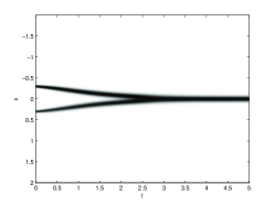
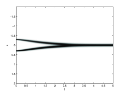
We notice that these parameters verify the properties in both examples 5.1 and 5.2. Therefore, we expect that the stationary solutions are concentrated on one or two Dirac masses that are symmetric with respect to the origin. As we observe in Figure 1, nε1superscriptsubscript𝑛𝜀1n_{\varepsilon}^{1} and nε2superscriptsubscript𝑛𝜀2n_{\varepsilon}^{2}, with (nε1,nε2)superscriptsubscript𝑛𝜀1superscriptsubscript𝑛𝜀2(n_{\varepsilon}^{1},n_{\varepsilon}^{2}) solution of the time-dependent problem 1 with the above parameters, concentrate in large time on a single Dirac mass at the origin, which is the mean value of the favorable traits in each zone in absence of migration. In this simulation, initially nε1superscriptsubscript𝑛𝜀1n_{\varepsilon}^{1} is concentrated on x=0.3𝑥0.3x=-0.3 and nε2superscriptsubscript𝑛𝜀2n_{\varepsilon}^{2} is concentrated on x=0.3𝑥0.3x=0.3.

Refer to caption
Refer to caption
Figure 1: Dynamics of the time-dependent problem 1 with parameters given in 35. In both figures, horizontally is time t𝑡t and vertically is trait x𝑥x. The gray layers represent the value of nε1superscriptsubscript𝑛𝜀1n_{\varepsilon}^{1}(left) and nε2superscriptsubscript𝑛𝜀2n_{\varepsilon}^{2}(right). Initially nε1superscriptsubscript𝑛𝜀1n_{\varepsilon}^{1} is concentrated on x=0.3𝑥0.3x=-0.3 and nε2superscriptsubscript𝑛𝜀2n_{\varepsilon}^{2} is concentrated on x=0.3𝑥0.3x=0.3. Due to migration both traits appear rapidly in the two patches, but in large time only one dominant trait persists. This point is the mean value of favorable traits in each patch in absence of migration.

Depending on the parameters of the model, one can also observe stability in large time of dimorphic situations. For instance, if we vary the values of ν1superscript𝜈1\nu^{1} and ν2superscript𝜈2\nu^{2} in 35 as follows

R1(x,I)=3(x+1)2I,R2(x,I)=3(x1)2I,ψ1(x)=ψ2(x)=1ν1=ν2=1,ε=.001,L=2,formulae-sequencesuperscript𝑅1𝑥𝐼3superscript𝑥12𝐼formulae-sequencesuperscript𝑅2𝑥𝐼3superscript𝑥12𝐼superscript𝜓1𝑥superscript𝜓2𝑥1formulae-sequencesuperscript𝜈1superscript𝜈21formulae-sequence𝜀.001𝐿2\begin{array}[]{c}R^{1}(x,I)=3-(x+1)^{2}-I,\quad R^{2}(x,I)=3-(x-1)^{2}-I,\quad\psi^{1}(x)=\psi^{2}(x)=1\\ \nu^{1}=\nu^{2}=1,\quad{\varepsilon=.001},\quad L=2,\end{array} (36)

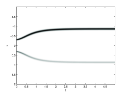
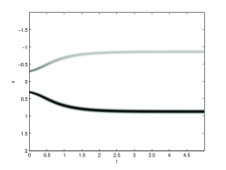
then nε1superscriptsubscript𝑛𝜀1n_{\varepsilon}^{1} and nε2superscriptsubscript𝑛𝜀2n_{\varepsilon}^{2}, with (nε1,nε2)superscriptsubscript𝑛𝜀1superscriptsubscript𝑛𝜀2(n_{\varepsilon}^{1},n_{\varepsilon}^{2}) solution of the time-dependent problem 1, concentrate in large time on two distinct Dirac masses, one of them more favorable to patch 111 and the second one more favorable to patch 222 (see Figure 2). We note indeed that, in absence of migration, the local optimal trait in patch 111 is x=1𝑥1x=-1 and in patch 222 is x=1𝑥1x=1. In presence of migration, the two initial traits appear immediately in the two patches and evolve to two points, one close to x=0.86𝑥0.86x=-0.86 and the other close to x=0.86𝑥0.86x=0.86.

Refer to caption
Refer to caption
Figure 2: Dynamics of the time-dependent problem 1 with parameters given in 36. In both figures, horizontally is time t𝑡t and vertically is trait x𝑥x. The gray layers represent the value of nε1superscriptsubscript𝑛𝜀1n_{\varepsilon}^{1}(left) and nε2superscriptsubscript𝑛𝜀2n_{\varepsilon}^{2}(right). In absence of migration, the local optimal trait in patch 111 is x=1𝑥1x=-1 and in patch 222 is x=1𝑥1x=1. Initially nε1superscriptsubscript𝑛𝜀1n_{\varepsilon}^{1} is concentrated on x=0.3𝑥0.3x=-0.3 and nε2superscriptsubscript𝑛𝜀2n_{\varepsilon}^{2} is concentrated on x=0.3𝑥0.3x=0.3. Due to migration both traits appear rapidly in the two patches, and evolve to two points close to 0.860.86-0.86 and 0.860.860.86.

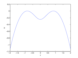
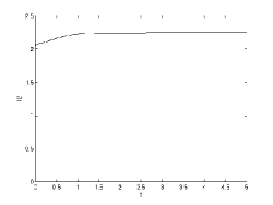
Does the above numerical solution converge in long time to the solution described by the algebraic constraints given in Theorem 1.2? The values of Iε1superscriptsubscript𝐼𝜀1I_{\varepsilon}^{1} and Iε2superscriptsubscript𝐼𝜀2I_{\varepsilon}^{2} are depicted in Figure 3 showing that both these quantities converge in long time to 2.252.252.25. We can also compute the value of H𝐻H at the final time step. As we observe in Figure 4, maxxH=0subscript𝑥𝐻0\max_{x}H=0 and the maximum is attained at the points x=.86𝑥.86x=-.86 and x=.86𝑥.86x=.86 which correspond to the positions of the Dirac masses in Figure 2. We can also compute numerically the weights of the Dirac masses at the final time step, to obtain

nε1(t=5)1.77δ(x+.86)+.48δ(x.86),nε2(t=5).48δ(x+.86)+1.77δ(x.86).formulae-sequencesuperscriptsubscript𝑛𝜀1𝑡51.77𝛿𝑥.86.48𝛿𝑥.86superscriptsubscript𝑛𝜀2𝑡5.48𝛿𝑥.861.77𝛿𝑥.86n_{\varepsilon}^{1}(t=5)\approx 1.77\,\delta(x+.86)+.48\,\delta(x-.86),\quad n_{\varepsilon}^{2}(t=5)\approx.48\,\delta(x+.86)+1.77\,\delta(x-.86).

One can verify that the above weights satisfy 1718.

Refer to caption
Refer to caption
Figure 3: Dynamics of the total populations: Iε1(t)superscriptsubscript𝐼𝜀1𝑡I_{\varepsilon}^{1}(t)(left) and Iε2(t)superscriptsubscript𝐼𝜀2𝑡I_{\varepsilon}^{2}(t)(right), using the parameters in 35. In both patches, the total population converges to a constant close to 2.252.252.25.
Refer to caption
Figure 4: The value of H(,Iε1(t),Iε2(t)H(\cdot,I_{\varepsilon}^{1}(t),I_{\varepsilon}^{2}(t) defined in 11, at time t=5𝑡5t=5.

Acknowledgments

The author benefits from a 2 year ”Fondation Mathématique Jacques Hadamard” (FMJH) postdoc scholarship. She would like to thank Ecole Polytechnique for its hospitality. She is also grateful to Clément Fabre for useful discussions.

References

  • [1] V. Bansaye and A. Lambert. Past, growth and persistence of source-sink metapopulations. Preprint.
  • [2] (MR2650800) G. Barles, S. Mirrahimi, and B. Perthame. Concentration in Lotka-Volterra parabolic or integral equations: a general convergence result. Methods Appl. Anal., 16(3):321–340, 2009.
  • [3] (MR2086750) J. Busca and B. Sirakov. Harnack type estimates for nonlinear elliptic systems and applications. Ann. Inst. H. Poincaré Anal. Non Linéaire, 21:543–590, 2004.
  • [4] (MR2151799) A. Calsina and S. Cuadrado. Stationary solutions of a selection mutation model: The pure mutation case. Mathematical Models and Methods in Applied Sciences, 15(7):1091–1117, 2005.
  • [5] (MR2290377) J. A. Carrillo, S. Cuadrado, and B. Perthame. Adaptive dynamics via Hamilton-Jacobi approach and entropy methods for a juvenile-adult model. Math. Biosci., 205(1):137–161, 2007.
  • [6] (MR2466448) N. Champagnat, R. Ferrière, and S. Méléard. From individual stochastic processes to macroscopic models in adaptive evolution. Stoch. Models, 24(suppl. 1):2–44, 2008.
  • [7] (MR2401952) N. Champagnat, R. Ferrière, and S. Méléard. Individual-based probabilistic models of adaptive evolution and various scaling approximations, volume 59 of Progress in Probability. Birkhäuser, 2008.
  • [8] (MR2793268) N. Champagnat and P.-E. Jabin. The evolutionary limit for models of populations interacting competitively via several resources. Journal of Differential Equations, 261:179–195, 2011.
  • [9] (MR1118699) M. G. Crandall, H. Ishii, and P.-L. Lions. User’s guide to viscosity solutions of second order partial differential equations. Bull. Amer. Math. Soc. (N.S.), 27(1):1–67, 1992.
  • [10] (MR2455473) L. Desvillettes, P.-E. Jabin, S. Mischler, and G. Raoul. On mutation-selection dynamics for continuous structured populations. Commun. Math. Sci., 6(3):729–747, 2008.
  • [11] (MR2076953) O. Diekmann. A beginner’s guide to adaptive dynamics. In Mathematical modelling of population dynamics, volume 63 of Banach Center Publ., pages 47–86. Polish Acad. Sci., Warsaw, 2004.
  • [12] O. Diekmann, P.-E. Jabin, S. Mischler, and B. Perthame. The dynamics of adaptation: an illuminating example and a Hamilton-Jacobi approach. Th. Pop. Biol., 67(4):257–271, 2005.
  • [13] (MR0714279) I. Eshel. Evolutionary and continuous stability. Journal of Theoretical Biology, 103(1):99 – 111, 1983.
  • [14] (MR1007533) L.C. Evans. The perturbed test function method for viscosity solutions of nonlinear PDE. Proc. R. Soc. Edinb. Sec. A, 111:359–375, 1989.
  • [15] S. A. H. Geritz, E. Kisdi, G. Mészena, and J. A. J. Metz. Evolutionarily singular strategies and the adaptive growth and branching of the evolutionary tree. Evol. Ecol, 12:35–57, 1998.
  • [16] S. A. H. Geritz, J. A. J. Metz, E. Kisdi, and G. Meszéna. Dynamics of adaptation and evolutionary branching. Phys. Rev. Lett., 78(10):2024–2027, Mar 1997.
  • [17] (MR2824978) P.-E. Jabin and G. Raoul. Selection dynamics with competition. J. Math. Biol., To appear.
  • [18] S. A. Levin. Community equilibria and stability, and an extension of the competitive exclusion principle. The American Naturalist, 104:413–423, 1970.
  • [19] S. Lion and M. van Baalen. Self-structuring in spatial evolutionary ecology. Ecology Letters, 11:277–295, 2008.
  • [20] (MR2765430) A. Lorz, S. Mirrahimi, and B. Perthame. Dirac mass dynamics in multidimensional nonlocal parabolic equations. Comm. Partial Differential Equations, 36(6):1071–1098, 2011.
  • [21] J. Maynard Smith and G. R. Price. The logic of animal conflict. Nature, 246:15–18, 1973.
  • [22] G. Meszéna, M. Gyllenberg, F. J. Jacobs, and J. A. J. Metz. Link between population dynamics and dynamics of Darwinian evolution. Phys. Rev. Lett., 95(7):078105.1–078105.4, Aug 2005.
  • [23] J. A. J. Metz, R. M. Nisbet, and S. A. H. Geritz. How should we define ”fitness” for general ecological scenarios? TREE, 7:198–202, 1992.
  • [24] S. Mirrahimi and P.E. Souganidis. A homogenization approach for the motion of motor proteins. Nonlinear Differential Equations and Applications NoDEA, To appear.
  • [25] (MR2492233) B. Perthame and G. Barles. Dirac concentrations in Lotka-Volterra parabolic PDEs. Indiana Univ. Math. J., 57(7):3275–3301, 2008.
  • [26] (MR2569885) B. Perthame and P. E. Souganidis. Asymmetric potentials and motor effect: a homogenization approach. Annales de l’Institut Henri Poincare (C) Non Linear Analysis, 26(6):2055 – 2071, 2009.
  • [27] (MR2506073) B. Perthame and P.E. Souganidis. Asymmetric potentials and motor effect: a large deviation approach. Arch. Ration. Mech. Anal., 193(1):153–169, 2009.
  • [28] (MR2781076) G. Raoul. Long time evolution of populations under selection and vanishing mutations. Acta Applicandae Mathematica, 114, 2011.
  • [29] T. W. Schoener. Resource partitioning in ecological communities. Science, 13:27–39, 1974.
  • [30] A. Szilágyi and G. Meszéna. Two-patch model of spatial niche segregation. Evolutionary Ecology, 23:187–205, 2009.