Fast Calculation of Calendar Time-, Age- and Duration Dependent Time at Risk in the Lexis Space

Abstract

In epidemiology, the person-years method is broadly used to estimate the incidence rates of health related events. This needs determination of time at risk stratified by period, age and sometimes by duration of disease or exposition. The article describes a fast method for calculating the time at risk in two- or three-dimensional Lexis diagrams based on Siddon’s algorithm.

Keywords: person-years method, Lexis diagram, Siddon’s algorithm.

1 Lexis diagram and person-years method

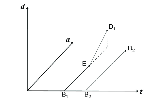
In epidemiology, oftentimes relevant events or outcomes simultaneously depend on different time scales: age of the subjects, calendar time and duration of an irreversible disease. In event history analysis, [5], a useful concept is the Lexis diagram, which is a co-ordinate system with axes calendar time $t$ (abscissa) and age $a$ (ordinate). The calendar time dimension sometimes is referred to as period. Each subject is represented by a line segment from time and age at entry to time and age at exit. Entry and exit may be birth and death, respectively, or entry and exit in a epidemiological study or trial. There are excellent and extensive introductions about the theory of Lexis diagrams (see for example [3], [4], [1] and references therein), which allows to be short here. When it comes to irreversible diseases, the commonly used two-dimensional Lexis diagram with axes in time and age direction may be generalized to a three-dimensional co-ordinate system with disease duration $d$ represented by the applicate (z-axis). If a subject does not get the disease during life time, the life line remains in the time-age-plane parallel to the line bisecting abscissa and ordinate. With other words, the life line for the time without disease points in the $(1,1,0)$ direction (where the triple $(t,a,d)$ denotes the co-ordinates in time, age and duration direction, respectively). However if at a certain point in time $E$ the disease is diagnosed, the life line changes its direction, henceforth pointing to $(1,1,1)$. The situation is illustrated in Figure 1. The life lines of two subjects are shown in the three-dimensional Lexis space. At time of birth (denoted $B_{n},~{}n=1,2$) both subjects are disease-free; both life lines go to the $(1,1,0)$ direction. The first subject gets the disease at $E$, and henceforth the life line is parallel to $(1,1,1)$ until death at $D_{1}$. The second subject remains without the disease for the whole life, which ends at $D_{2}$.

Figure 1: Three-dimensional Lexis diagram with two life lines. Abscissa, ordinate and applicate represent calendar time $t$, age $a$ and duration $d$, respectively. The life lines start and end at birth $B_{n}$ and death $D_{n},~{}n=1,2.$ The first subject gets the disease at $E$. Then, the life line changes its direction. The second subject does not get the disease, the corresponding life line remains in the $t$-$a$-plane.

In order to measure the frequency of events in a population, such as onset of a chronic disease, the person-years methods records the number of people who are affected and the time elapsed before the event occurs. The person-years incidence rate $\lambda$ is estimated by

$$\lambda=\frac{e}{m},$$ (1)

where $e$ is is the number of events and $m$ is the number of person-years at risk [7, p. 250ff]. Calendar time and age often are important determinants for occurrence of events and have to be taken into account. This usually is achieved by dividing the subjects’ time spent in the study into calendar time and age groups. Let $e_{ij}$ be the number of events taking place while subjects are in time and age group $(i,j).$ Furthermore, let $m_{ij}$ be the total time at risk spent in this group, then Equation (1) becomes

$$\lambda_{ij}=\tfrac{e_{ij}}{m_{ij}}.$$

In the planar Lexis diagram it is clear, how the time at risk $m_{ij}$ can be obtained. Let the time and age group $(i,j)$ be defined by Cartesian product $S_{ij}:=[t_{i-1},t_{i})\times[a_{j-1},a_{j})$. Each subject whose life line intersects with the rectangle $S_{ij}$ contributes by its time at risk in $S_{ij}$. To be precise, $m_{ij}$ is the sum of all the subjects’ times at risk spent in $S_{ij}$:

$$m_{ij}=\sum_{n=1}^{N}\ell^{(n)}_{ij},$$ (2)

where $\ell^{(n)}_{ij}$ is the time at risk of subject $n,~{}n=1,\dots,N,$ in the rectangle $S_{ij}.$

Again, these ideas can be generalized to three-dimensional case: Then, $e_{ijk}$ is the number of events taking place in the rectangular hexahedron

$$S_{ijk}:=[t_{i-1},t_{i})\times[a_{j-1},a_{j})\times[d_{k-1},d_{k}).$$

For the times at risk $m_{ijk}$ it holds

$$m_{ijk}=\sum_{n=1}^{N}\ell^{(n)}_{ijk},$$ (3)

where $\ell^{(n)}_{ijk}$ is the time at risk of subject $n$ in volume element $S_{ijk}.$

Given a certain study population of size $N$, the question arises how the subjects’ contributions $\ell^{(n)}_{ijk}$ to the overall time at risk $m_{ijk}$ spent in $S_{ijk}$ can be calculated. Since $N$ may be large (up to several thousand), some attention should be paid to computation time.

The solution is straightforward by noting that the question is very similar to the problem of following a radiological path through a voxel grid in tomography or raytracing in computer graphics. For both fields, tomography and raytracing, there is an ongoing research effort to efficiently discretize continuous lines (radiological paths or rays of light). This article has been inspired by the seminal work of Siddon, [6].

2 Intersecting life lines with voxels in the Lexis diagram

Since the algorithm presented in this section is motivated from the field of computer tomography, some of the terminology is useful. Typically one of the sets $S_{ijk}$ resulting from a partition of a rectangular hexahedron (right cuboid) into congruent volume elements, is called a voxel. The six faces of each voxel are subsets of two adjacent planes parallel either to the $t$-$a$-plane, $a$-$d$-plane or $t$-$d$-plane. Hence, the voxel space comes along with a set of equidistant, parallel planes which are perpendicular to the abscissa, ordinate or applicate and which are defined by the union of all voxel faces. These planes play a crucial role in the algorithm.

In this article all voxels $S_{ijk}$ are considered to be cubical, with all edges having the length $t_{r},~{}t_{r}>0:$

$$S_{ijk}:=\left[t_{r}\cdot\left(i-1\right),~{}t_{r}\cdot i\right)\times\left[t_{r}\cdot\left(j-1\right),~{}t_{r}\cdot j\right)\times\left[t_{r}\cdot\left(k-1\right),~{}t_{r}\cdot k\right).$$ (4)

These voxels form a grid where the life lines of all subjects in the study are sorted into. As a consequence of cubical voxels, the temporal resolution with respect to calendar time, age and duration is the same. However, generalization to partitions usings rectangular voxels with height, length and depth being different is easily possible.

The main idea for calculating the $\ell^{(n)}_{ijk}$ in the life line ${\cal L}_{n}$ of subject $n$ starting at entry point $B_{n}:=(t^{(n)}_{0},a^{(n)}_{0},d^{(n)}_{0})$, ending at exit point $D_{n}:=(t^{(n)}_{1},a^{(n)}_{1},d^{(n)}_{1})$, is the parameterization in the form

$${\cal L}_{n}:~{}B_{n}+\alpha\cdot(D_{n}-B_{n}),~{}\alpha\in[0,1].$$

Note, that $t^{(n)}_{1}-t^{(n)}_{0}=a^{(n)}_{1}-a^{(n)}_{0}=d^{(n)}_{1}-d^{(n)}_{0}=:\Delta t^{(n)}.$ Using this parameterization, all parameters $\alpha^{(n)}\in[0,1]$ are calculated where an intersection with a voxel face takes place. Since the voxels are arranged in a regular grid, intersecting one of the voxel faces is equivalent with intersecting one of the $t$-$a$-, $a$-$d$- or $t$-$d$-planes formed by the union of all voxel faces mentioned above. Hence, we calculate the intersections with these planes.

Let us start with the $a$-$d$-planes (perpendicular to the $t$-axis): all those $\alpha^{(n)}_{t}$ where an intersection with an $a$-$d$-plane occurs are given by

$$\alpha^{(n)}_{t}(u)=\frac{u\cdot t_{r}-(t^{(n)}_{0}~{}\%~{}t_{r})}{\Delta t^{(n)}},~{}u=1,\dots,U^{(n)},$$

where $\%$ is the modulo-operator and $U^{(n)}$ denotes the number of intersected $a$-$d$-planes:

$$U^{(n)}=\left\lfloor\nicefrac{{t^{(n)}_{1}}}{{t_{r}}}\right\rfloor-\left\lfloor\nicefrac{{t^{(n)}_{0}}}{{t_{r}}}\right\rfloor.$$

Similar formulas hold for those $\alpha^{(n)}_{a}(v),~{}v=1,\dots,V^{(n)},$ and $\alpha^{(n)}_{d}(w),~{}w=1,\dots,W^{(n)},$ where ${\cal L}_{n}$ intersects the $t$-$d$- or $t$-$a$-planes, respectively. Now define the set

$$A_{n}:= \{\alpha^{(n)}_{t}(u)~{}|~{}u=1,\dots,~{}U^{(n)}\}$$

$$\cup \{\alpha^{(n)}_{a}(v)~{}|~{}v=1,\dots,~{}V^{(n)}\}$$

$$\cup \{\alpha^{(n)}_{d}(w)~{}|~{}w=1,\dots,W^{(n)}\},$$

which contains those $\alpha^{(n)}\in[0,1]$ where an intersection occurs. Note that the three sets on the right-hand side of Equation (2) are not necessarily disjoint. Multiple values occur if an intersection happens to be on an edge or vertex of a voxel. Let $A^{\star}_{n}:=A_{n}\cup\{0,~{}1\}$ be ordered ascendingly $A^{\star}_{n}=\{\alpha^{(n)}(p)~{}|~{}p=1,\dots,P^{(n)}\}$ with $0=\alpha^{(n)}(1)<\dots<\alpha^{(n)}(P^{(n)})=1.$ For calculating the $\ell^{(n)}$ and the associated voxel indices $i,j,k,$ we have following algorithm:

1. For each subject $n,~{}n=1,\dots,N,$ calculate the set $A^{\star}_{n}$ as above and sort the elements $\alpha^{(n)}(p),~{}p=1,\dots,P^{(n)},$ in ascending order.

2. For $p=1,\dots,P^{(n)}$ set

   $$(i_{p},j_{p},k_{p}):=\left\lfloor\frac{B_{n}+\alpha^{(n)}(p)\cdot(D_{n}-B_{n})}{t_{r}}\right\rfloor,$$ (6)

   where the division is taken componentwise.

3. Then, calculate

   $$\ell^{(n)}_{i_{p}j_{p}k_{p}}=\left(\alpha^{(n)}(p+1)-\alpha^{(n)}(p)\right)\cdot\Delta t^{(n)},~{}p=1,\dots,P^{(n)}-1.$$ (7)

For each voxel $(i,j,k)$ summing up all the times $\ell^{(n)}_{ijk},~{}n=1,\dots,N,$ by Equation (3) yields the time at risk $m_{ijk}$ in period-, age- and duration class $(i,j,k),$ which can be used in the person-years method.

The idea of calculating the intersection points with the voxel faces goes back to Robert L. Siddon. The algorithm proposed by Siddon has been developed for raytracing in tomography, where several millions of paths have to be computed to form a radiological image. While the implementation provided with this article is not tuned for efficiency, remarkable speeding up is possible [2]. The execution of 500 runs of an R (The R Foundation for Statistical Computing) implementation of the algorithm with the data of 200 patients (equivalent to a total of $10^{5}$ patients) on a 2.6 GHz personal computer takes 92 seconds. The (simulated) patient data set is described in more detail in the next section.

3 Examples

An implemtentation of the method in this article has been tested with simulated patient data. A study population of 200 subjects with entry age 55 to 85 born between 0 and 15 (TUs) suffering from a chronic disease for 3 to 15 TUs at is the time of entry is assumed to have the mortality rate

$$m(a,d)=\exp(-10+0.1\cdot a)\cdot(1+0.1\cdot d).$$

Exit from the study is assumed to be only due to death (no censoring). The aim is to unfold the mortality rate from these patient data.

For setting up the data set, following code has been used:

for(patNr in 1:200){
   thisPatInAge       <- runif(1, 55, 80)
   thisPatBirth       <- runif(1,  0, 15)
   thisPatDuration    <- runif(1,  3, 15)

   F                  <- fct_F(thisPatInAge, thisPatDuration)
   thisPatDeathAge    <- round(   which.min(runif(1) > F) + thisPatInAge
                               + (runif(1) - 0.5), 3)
   patMatrix[patNr, ] <- c(thisPatBirth, thisPatInAge, thisPatDuration,
                             thisPatDeathAge)
}

For the simulation of the age of death, inverse transform sampling is used:
(which.min(runif(1) > F)). Therefor the cumulative distribution function $F(t~{}|~{}a_{0},d_{0})$ for someone who enters the study at age $a_{0}$ and having got the disease for $d_{0}$ TUs is calculated in the function fct_F:

$$F(t~{}|~{}a_{0},d_{0})=1-\exp\left(-\int_{0}^{t}m(a_{0}+\tau,d_{0}+\tau)\mathrm{d}\tau\right).$$

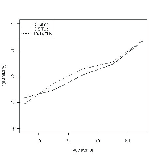
If the alorithm is applied to this data set with $t_{r}=5,$ it is possible to estimate the mortality rate $m(a,d)$ by the person-years method. The result is shown in Figure 2.

Figure 2: Age- and duration specific mortality as estimated by the person-years method.

4 Conclusion

This article is about an extension of the person-years when period-, age- and duration-effects occur. The method to calculate the time at risk is based on raytracing techniques used in tomography and provides a fast way to follow the individual life lines of subjects in the Lexis diagram. The algorithm is able to treat two cases

1. calculate the time at risk for newly incident cases, and

2. calculate the time at risk, where the time elapsed after an event (e.g. duration since onset of a disease) is relevant.

In the first case, the life lines are located in the $t$-$a$-plane, in the second the life lines are pointing to the $(1,1,1)$ direction. The later case is important, when the duration is a covariable. This might be the case in late sequalae or mortality after having got a disease. Similarly, by interpreting the applicate axis (z-axis) as duration of exposure to a risk factor, the time at risk depending on period, age and duration of exposure can be calculated.

In large populations or register data ($\log_{10}N>5$ , times at risk are usually estimated by a formula going back to Sverdrup, [1, Sect. 3.2.]. It is noted that using the method described in this article, estimation is no longer necessary, because given entry and exit times of the subjects, calculation of times at risk is possible at feasible computational expense.

References

- [1] Bendix Carstensen. Age-Period-Cohort Models for the Lexis Diagram. Statistics in Medicine, 26(15):3018–3045, 2007.
- [2] Mark Christiaens, Bjorn De Sutter, Koen De Bosschere, Jan Van Campenhout, and Ignace Lemahieu. A fast, cache-aware algorithm for the calculation of radiological paths exploiting subword parallelism. In Journal of Systems Architecture, Special Issue on Parallel Image Processing, 1998.
- [3] Niels Keiding. Statistical interference in the lexis diagram. Philosophical Transactions of the Royal Society London A, 332:487–509, 1990.
- [4] Niels Keiding. Age-specific incidence and prevalence: a statistical perspective. Journal of the Royal Statistical Society A, 154:371–412, 1991.
- [5] Niels Keiding. Event history analysis and the cross-section. Statistics in Medicine, 25(14):2343–2364, 2006.
- [6] Robert L. Siddon. Fast Calculation of the Exact Radiological Path for a Three-Dimensional CT Array. Medical Physics, 12(2):252–255, 1985.
- [7] Mark Woodward. Epidemiology: Study Design and Data Analysis. Texts in statistical science. Chapman & Hall/CRC, 2005.